Characterizing the spatial and temporal variation of the land surface temperature hotspots in Wuhan from a local scale

ABSTRACT

Land Surface Temperature (LST) derived from space-borne Thermal-infrared (TIR) sensors is a key parameter of urban climate studies. Current studies are inefficient to capture the spatial and temporal variations of LST for only one snapshot adopted at one time. Focusing on the characterization of the spatial and temporal of LST variations at local scales, the latent patterns, and morphological characteristics are extracted in this study. Technically, sixteen MODerate-resolution Imaging Spectroradiometer (MODIS) eight-day synthesized LST products (MYD11A2) in 2002, 2007, 2012, and 2017 are employed. First, the non-parametric Multi-Task Gaussian Process Model (MTGP) is used to extract the smooth and continuous Latent LST (LLST) patterns using one LST subset and its temporally adjacent images. Second, the Multi-Scale Shape Index (MSSI) is then applied to quantify the morphological characteristics at the optimal scale. Then, the LLST patterns and MSSI maps are clustered into multiple spatial categories. The specific clusters with the highest LLST and MSSI values are considered as local LLST hotspots. The Hotspots Weighted Mean Center (HSWMC) and standard deviation ellipse are adopted to further investigate the spatiotemporal change of hotspots orientation, direction, and trajectories. Results revealed that Impervious Surfaces (IS) composition is the most significant external forcing of local LST anomalies. The configuration factors (e.g., shape index, aggregation index) also have a noticeable local warming effect. This study represents a latent pattern and morphology-based framework for LST hotspots spatial and temporal variations characterization, catering to the zoning and grading strategies in urban planning.

KEYWORDS:

• Land Surface Temperature (LST)
• latent pattern
• morphology
• spatiotemporal variation
• Gaussian process

1. Introduction

The unprecedented development of society and accelerated urbanization have prominent impacts on the energy balance, precipitation, air quality, local biodiversity, surface runoff, carbon sequestration (Chen et al. 2017; Stewart and Oke 2012; Huang and Wang 2020; Nistor 2019). One of the major concerns of urbanization is its effect on the urban thermal environment. The Urban Heat Island (UHI) effect is one of the most common factors affecting urban climate, urban life quality, and urban ecological diversity (Chen et al. 2017; Dos Santos et al. 2017; Trinder and Liu 2020; Shao et al. 2020; Liu, Huang, and Yang 2020; Yang et al. 2020). The magnitude of UHI can achieve 12°C under calm and clear weather conditions (Wang, Zhan, and Guo 2016). Numerous systematic studies of LST have been carried out for identifying the meteorological process within urban areas. In this context, UHI can be further distinguished as Urban Boundary Layer (UBL) and Urban Canopy Layer (UCL) heat island (Oke 1988; Wang, Zhan, and Guo 2016). When urban Land Surface Temperature (LST) is emphasized in the studies, the UCL heat island can be identified as Surface Urban Heat Island (SUHI). SUHI is closely bound up with urban climate at macro, meso, and micro scales, governing the energy balance and meteorological pattern within UCL. LST maps derived from satellite remotely sensed images have been the most essential materials in SUHI studies for its broad coverage, frequency revisit, and various resolutions (Yang et al. 2013).

Most previous studies are inclined to adopt only one snapshot at a specific time to represent the LST spatial pattern (Wang, Zhan, and Guo 2016; Liu et al. 2018; Liu et al. 2019a; Yang et al. 2019). However, it is essential to consider temporal nonstationarity of LST and generate LST data with typical spatial-temporal patterns in a specific time range (Wang, Zhan, and Guo 2016; Liu et al. 2019a). On the one hand, LST possesses the arresting temporal nonstationarity, as generally considered as Diurnal Temperature Cycle (DTC) (Weng and Fu 2014b), Annual Temperature Cycle (ATC) (Weng and Fu 2014a), and interannual variations (Liu et al. 2019b). On the other hand, the meteorological and hydrological conditions are complicated and capricious, causing distinct-different LST patterns in temporally adjacent satellite images (Liu et al. 2018). Therefore, no matter for SUHI mechanism investigation or spatial-temporal pattern exploration, it can be misleading as conducting SUHI mapping from a static perspective (Weng and Fu 2014b; Zhou et al. 2018). The direct comparison of remotely sensed LST maps derived under different atmospheric and hydrological conditions as neglecting the temporal nonstationarity of LST is defective (Zhou et al. 2018; Liu et al. 2018).

Studies aimed at generating smooth and continuous LST surfaces are well documented, e.g., unimodal Gaussian surface (Streutker 2003), non-parametric kernel surface (Rajasekar and Weng 2009), and spatial and temporal fusion (Shen et al. 2016). Among them, the Multi-Task Gaussian Process (MTGP) model is introduced by Wang et al. (Wang, Zhan, and Guo 2016) for extracting the Latent pattern of LST (LLST) from raw remotely sensed LST imageries. The LLST is a smooth and continuous surface depicting the latent spatial pattern of LST hidden in the noisy raw satellite-derived LST maps (Liu et al. 2018; Wang, Zhan, and Guo 2016). The continuous LLST patterns without noises and null observations are deemed to support explore the local LST anomalies better. Furthermore, as integrating one raw LST map with three temporally adjacent imageries in a month, the extracted LLST datasets by MTGP are capable to depict the monthly typical LST patterns (Liu et al. 2018; Wang, Zhan, and Guo 2016).

Besides, conventional indicators measuring UHI intensity are incompetent to delineate the LLST patterns for the inherent neglect toward LST spatial non-stationarity within cities (Liu et al. 2018; Wang, Zhan, and Guo 2016; Li et al. 2018; Zhou et al. 2018). The morphological characteristics, quantified by Multi-Scale Shape Index (MSSI) (Wang, Zhan, and Guo 2016), are quite competent to portray LLST patterns at the optimal scale by characterizing local LST variation. Besides the capability of characterizing local LLST patterns, MSSI is an efficient indicator to explore the LST anomalies at a local scale. Such local anomalies with higher LST and MSSI values compared to surroundings are considered as local LLST hotspots in this study.

The intensification and expansion of Impervious Surfaces (IS) accompanied by urbanization are claimed to be responsible for local warming (Kuang et al. 2015; Yang et al. 2019; Li et al. 2017). IS, mainly composed of asphalt, concrete, pebbles, and bricks, can modulate evapotransporative features and radiation fluxes of land surfaces (Kuang et al. 2019; Yang et al. 2019; Kuang, Li, and Hamdi 2020), thus amplifying UHI intensity. A large body of researches has attempted to identify the associations between local LST anomalies/UHI effects with IS composition and configuration (Chen et al. 2014; Li et al. 2017; Liu, Peng, and Wang 2017). Numerous metrics have been introduced in FRAGSTATS software to quantify the landscape composition and configuration features (Chen et al. 2014; Li et al. 2017; Mcgarigal 1995). The composition and edge metrics are examined to be the most critical factors in the characterization of UHI-associated LST indication in the metropolitan area of Beijing (Chen et al. 2014). Yet less attention has been paid to the impacts of landscape metrics’ temporal variations on the latent LST dynamics. Besides, little is known about the impacts of IS configuration in local LST anomalies characterization. Hence, it is necessary to implement further examinations on the associations between spatiotemporal LST dynamics and landscape metrics.

In this study, the local LLST hotspots are denoted as the specific spatial clusters with the highest LLST and MSSI values categorized by Gaussian Mixture Model (GMM), the claimed robust and effective method in space and time-series differentiation (Zhao et al. 2016; Aghabozorgi, Shirkhorshidi, and Wah 2015). Furthermore, the orientation, dispersion degree, and moving trajectories can provide crucial implications for local thermal environment mechanisms exploration and the identification of urban planning implementations toward UHI mitigation (Weng et al. 2019; Qiao et al. 2019). In this study, the Hotspots Weighted Mean Center (HSWMC) (Qiao et al. 2019) is introduced to reveal the moving trajectories of barycenter of local hotspots. Besides, the orientation and dispersion degree of local hotspots are reflected by the Standard Deviation Eclipse (SDE) (Xu et al. 2018).

Specifically, by taking Wuhan as a case study, this study aims at characterizing local LST anomalies to facilitate urban planning. The 8-day synthesized MODerate-resolution Imaging Spectroradiometer (MODIS) LST products (MYD11A2) are adopted to represent the monthly typical LST patterns. First, the heuristic MTGP is responsible for deriving smooth LLST without noise and missing observations due to cloud contamination (Wang, Zhan, and Guo 2016; Liu et al. 2019a). MSSI then quantifies the morphological features of LLST patterns. To further carter the need for zoning and grading in urban planning practices, the LST differentiation is subsequently conducted by commonly-used model-based Gaussian Mixture Model (GMM) clustering (ZZhao et al. 2016). The particular objectives of this study are to investigate (1) the typical LLST patterns from 2002 to 2017 with five years internal and the spatial and temporal variations of LLST patterns, (2) the principle direction of hotspots expansion in the whole period by HSWMC, (3) the orientation, clustering (or dispersion) degree by SDE, (4) the impacts of IS configuration and composition on the local LST anomalies are quantified in 2002, 2007, 2012, and 2017 are using Random Forest (RF). The detailed techniques and discussions are provided in the following sections.

2. Study area and materials

2.1. The study area

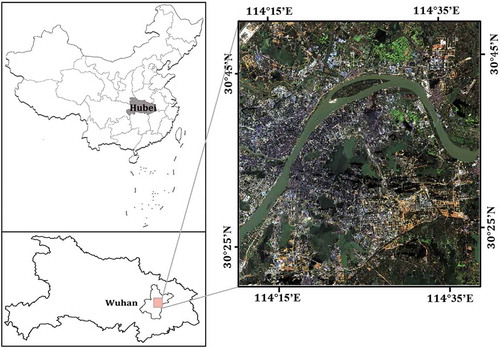
Wuhan, one of the biggest cities in central China with prominent growing rates, is selected as the study case. Wuhan possesses a typical subtropical monsoon climate, typified by the time-span of summer as 135 days. As shown in Figure 1, the specific study area is $49\mathrm{k}\mathrm{m}\times 44\mathrm{k}\mathrm{m}$ covering the main part of the central downtown area and fractional rural surroundings with heterogeneous landscapes, e.g., impervious surface, vegetations, and water bodies. The spatial extent of this area is ${30}^{\circ }{47}^{\prime }32{ }^{\prime \prime }\mathrm{N}$, ${114}^{\circ }{12}^{\prime }01{ }^{\prime \prime }\mathrm{E}$ (upper-left) to ${30}^{\circ }{20}^{\prime }19{ }^{\prime \prime }\mathrm{N}$, ${114}^{\circ }{38}^{\prime }32{ }^{\prime \prime }\mathrm{E}$ (lower-right).

Figure 1. The study area was represented by the Landsat 8 OLI image (RGB) on 24 October 2017

2.2. Datasets

2.2.1. MODIS land surface temperature (LST) products

Enormous previous studies taking Wuhan as a case have revealed that July and August are the hottest months in a year (Liu et al. 2018; Shen et al. 2016). Thus, for better investigation of local LST anomalies within Wuhan, MODIS/Aqua 1-km gridded LST products (MYD11A2) acquired at 13:30 are employed in this study. MODIS LST products are produced by the generalized split-window algorithm with an accuracy better than 1°C (0.5°C in most cases) (Wan 2008, 2014). Specifically, for analyzing the spatial and temporal variations of LST from 2002 to 2017, 16 MODIS 8-day synthesized LST subsets (four in a year) in July and August during this period are downloaded waiting for further process.

For better analyzing the time-series LST data on the same basis, LST products shall be pre-screened according to meteorological data for two reasons: (1) the LST data acquired by space-borne sensors are greatly affected by atmospheric water vapor, and cloud contamination (Shen et al. 2016; Wan 2014), (2) LST may fluctuate dramatically in response to the variations of atmospheric and hydrological conditions in temporally adjacent days (Liu et al. 2018; Weng and Fu 2014b). Since spatially-temporally dense in-site observed meteorological data are not available, the daily-average meteorological data is collected from the website (www.weatherground.com) for data filtering. The weather stability measured by the adapted Pasquill-Gifford scale ensures meteorological and hydrological conditions are stable during the data acquirement (Wang, Zhan, and Guo 2016; Tomlinson et al. 2012). The specific class of weather stability measured by the adapted Pasquill-Gifford scale are D (Neutral), E (Slightly Stable), F (Moderately Stable), and G (Extremely Stable). In each year, the LLST pattern has been derived mainly from the dominant LST subset acquired under the ideal weather condition and the sharing information from three other temporally adjacent LST subsets. The detailed information of selected dominant LST subsets is reported in Table 1.

Table 1. Selected LST products and corresponding weather information

Selected date of the dominant subset	8-day average Temp. (°C)	8-day average relative humidity	Average wind speed (m/s)	Adapted Pasquill-Gifford stability class	Dates of 3 auxiliary subsets
2002/07/12	34.6	67.5	1.2	G	2002/07/04 2002/07/28 2002/08/04
2007/07/28	32.8	70.9	2.3	F	2007/07/20 2007/08/04 2007/08/12
2012/07/21	35.1	72.7	1.8	G	2012/07/05 2012/07/13 2012/07/29
2017/07/20	35.3	69.6	2.0	G	2017/07/20 2017/08/13 2017/08/21

2.2.2. Impervious surfaces maps

In this study, the 30-meter IS maps published by Gong, Li, and Zhang (2019) are used to depict the spatial and temporal distribution of IS in Wuhan from 2002 to 2017. Such IS maps are derived mainly from 30-meter Landsat images and refined using Nighttime Light (NTL) data (Gong, Li, and Zhang 2019). The accuracy of IS extraction of this dataset is claimed to be better than 93% in most cases. More details of this IS maps dataset can be checked in the literatures (Li and Gong 2016; Li, Gong, and Liang 2015; Gong, Li, and Zhang 2019). To be consistent with the resolution of LST data, the landscape metrics are calculated in 500 m$\times$500 m grids in FRAGSTATS.

3. Methodology

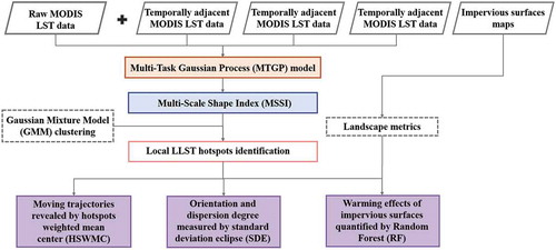
As shown in Figure 2, the latent and monthly typical LLST patterns are extracted from raw MODIS LST products using the MTGP model, and the morphological features are characterized by MSSI. Then the specific spatial clusters categorized by GMM with the highest LLST and MSSI values are identified as the local LLST hotspots. Furthermore, the orientation, dispersion, and moving trajectories are analyzed using HSWMC and SDE. Finally, the local warming effect of IS is quantified using RF in 2002, 2007, 2012, and 2017.

Figure 2. The technical flow of this study

3.1. MTGP for latent LST (LLST) pattern extraction

The Latent LST (LLST) pattern is defined as a continuous and smooth surface at the whole region scale without noises and null observations in previous studies (Liu et al. 2018; Wang, Zhan, and Guo 2016; Liu et al. 2019). The LLST pattern, as continuous information, is claimed to support pattern recognition more competent (Wang, Zhan, and Guo 2016). Specifically, the non-parametric heuristic MTGP model is adopted to generate a monthly typical LLST pattern by coupling four temporally adjacent LST maps. The MTGP possesses the merits of filtering noises and filing observation deficiencies without intentional interventions and controlling local variations without distorting overall diversity. Furthermore, MTGP is also capable of generating more detailed LLST patterns for more effective recognition by interpolating into finer resolution.

MTGP, a non-parametric machine learning method (Bonilla 2008), extract the LLST using the information in the original LST map and auxiliary information of temporally adjacent images. The observed time-series LST dataset is represented as $D=\left\{\left(x_i,t_{ij}\right)|i=1,\dots ,n;j=1,\dots m\right\}$, in which $x_i$ denotes the i-th location index in dimensional space $R^d$, and $t_{ij}$ denotes the observation at location $x_i$ in the j-th image. Besides, $n$ is the number of pixels on one image, and $m$ is the number of images applied in the model. The Gaussian Process (GP) model generalizes the extract form into an infinitely long vector ${\left[f_1,\dots ,f_n\right]}^T$, among which any finite set of the vector is jointly Gaussian. The model $f\left(x\right)\text{~}GP\left(m\left(x\right),K^f{K}^x\right),$ is completely defined by the mean function $m\left(x\right)$ and the covariance function. $K^f$ is the covariance function stating the inter-task information between the images, while $K^x$ is the covariance function explaining the intra-task information inside one snapshot.

Any mean value $\overline{f^{\ast }}$ of LLST is predicted by

(1) $\overline{f^{\ast }}=m\left(x^{\ast }\right)+{\left(k^f\otimes k^x\left(x^{\ast },x\right)\right)}^T{\left(K^f\otimes K^x+\otimes I\right)}^{-1}\left(t-m\left(X\right)\right)$(1)

where $\otimes$ denotes the Kronecker product of matrices or vectors and $\mathrm{\Delta }$ is a diagonal matrix to record noise ${\sigma }^2$.

3.2. Morphology of LLST patterns

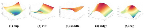
Numerous parameters are available for quantifying the intensity or magnitude, spatial extent, orientation, and position of SUHI (Wang, Zhan, and Guo 2016; Zhou et al. 2011; Li et al. 2018). However, these parameters limited by the global scale “urban-rural” assumption are deficient for capturing the locally spatial pattern of LLST (Wang, Zhan, and Guo 2016). The local variations of LLST are affected by surroundings, thus presenting a variety of shapes. Therefore, it is feasible to investigate spatial and temporal variations of SUHI utilizing diverse morphological characteristics at local scales. Multi-Scale Shape Index, a morphological index enriching the descriptive parameter system of SUHI, is proposed by Wang et al. (Wang, Zhan, and Guo 2016). MSSI is a normalized index quantifying the morphological characteristics of SUHI, i.e., cups, ruts, saddles, ridges, and caps, as shown in Figure 3.

Figure 3. The surface morphological features of LLST patterns (Wang, Zhan, and Guo 2016; Liu et al. 2018)

Specifically, the LST pattern $\mathrm{f}\left(s\right)$ is projected to the scale-space (Koenderink and van Doorn 1992) $S$ through the formula below:

(2) $S\left(f\left(s\right),\sigma \right)=f\left(s\right)\text{setbox}\$\times \$\text{t}o\text{wd}\text{hss}\$÷\$\text{hss}\text{box}k\left(s-u,\sigma \right)=\underset{0}{\overset{s}{\int }}f\left(u\right)k\left(s-u,\sigma \right)du$(2)

in which $k\left(,\right)$ indicates the Gaussian kernel, and $\sigma$ as the convolution scale of location $u$ on surface $s$. Every point in the original image corresponding to the convolution kernel center would shift as the kernel smoothing at different scales. The fluctuation intensity of the original image thus gets compressed. The feature scale is generated by maximizing the normalized drift distance at a different convolution scale $\sigma$. The normalized distance is calculated by

(3) $d=\frac{D\left(f,\sigma \right)}{\sigma }=\frac{S\left(f,\sigma \right)-f^2}{\sigma }$(3)

The original shape index (SI) (Koenderink and van Doorn 1992) is calculated through

(4) $SI=\frac{2}{\pi }arctan\frac{{\kappa }_2+{\kappa }_1}{{\kappa }_2-{\kappa }_1},SI\in \left[-1,1\right]$(4)

where ${\kappa }_1$ and ${\kappa }_2$ (${\kappa }_1\ge {\kappa }_2$) represent the principal curvatures generated from a noiseless continuous LLST surface. The value of $SI$ indicates the protruding and depression of a particular pixel. Specifically, these shapes can be described as cups, ruts, saddles, ridges, and caps.

3.3. Hotspots designation by Gaussian Mixture Model (GMM) clustering

Gaussian Mixture Model (GMM), a model-based unsupervised method recognized as effective and robust in spatial and temporal clustering (ZZhao et al. 2016; Warren Liao 2005; Aghabozorgi, Shirkhorshidi, and Wah 2015), is adopted to perform spatial differentiation on LLST for catering the zoning and grading strategy in urban planning to better bridge the gap between thermal environment studies and SUHI mitigation planning practice.

The specific cluster with the highest LST and MSSI values is denoted as local hotspots of LLST patterns (Liu et al. 2018; Hao et al. 2016). Many studies have investigated that local hotspots of LST are inclined to locate in the built-up surfaces within downtown areas and bare lands in urban surroundings (Hao et al. 2016; Wang, Zhan, and Guo 2016; Wang et al. 2016). By mining the LLST spots, the global “urban-rural” dichotomy can be refined into the consideration of local LST diversity, which shall provide an initiatory spatial extent require planning actions.

3.4. Hotspots weighted mean center (HSWMC) analysis

In order to represent the spatial and temporal variations of LLST, the barycenter is adopted to indicate the spatiotemporal trajectories of hotspots (Xu et al. 2018). In this study, the barycenter is modified as the hotspots weighted mean center (HSWMC) by considering LLST values. The coordinates spatialization of HSWMCs is calculated as:

(5) $\left\{\begin{array}{c}\bar{x}=\frac{{\sum }_{i=1}^n{m}_i{x}_i}{{\sum }_{i=1}^n{m}_i}\\ \bar{y}=\frac{{\sum }_{i=1}^n{m}_i{y}_i}{{\sum }_{i=1}^n{m}_i}\end{array}\right.$(5)

where $\bar{x},\bar{y}$ are the coordinates of calculated HSWMC $x,y$ are the coordinates of a specific pixel in hotspots. $i$ represents the $i$th pixel, and $m_i$ is the heating magnitude of $i$th pixel, i.e., the difference between the LLST value of $i$th pixel and mean LLST values out of hotspots. The calculation of HSWMCs of time-series LLST patterns reveals the overall trends of hotspots within Wuhan city, which can support the dynamic variations of the local thermal environment.

3.5. Orientation and dispersion of LLST

The weighted Standard Deviational Ellipse (SDE) is employed to further measure the orientation, direction, and spatial and temporal development of LLST hotspots (Xu et al. 2018). The azimuth of SDE is calculated as:

(6) $\mathrm{t}\mathrm{a}\mathrm{n}\theta =\frac{\left(\sum _{i=1}^n{\omega }_i^2{\tilde{x}}_i^2-\sum _{i=1}^n{\omega }_i^2{\tilde{y}}_i^2\right)+\sqrt{{\left(\sum _{i=1}^n{\omega }_i^2{\tilde{x}}_i^2-\sum _{i=1}^n{\omega }_i^2{\tilde{y}}_i^2\right)}^2-4{\left(\sum _{i=1}^n{\omega }_i^2\widetilde{x_i}\widetilde{y_i}\right)}^2}}{2\sum _{i=1}^n{\omega }_i^2\widetilde{x_i}\widetilde{y_i}}$(6)

(7) $\left\{\begin{array}{c}\widetilde{x_i}=x_i-\bar{x}\\ \widetilde{y_i}=y_i-\bar{y}\end{array}\right.$(7)

where $\theta$ is the azimuth of the SDE, representing the clockwise angle from North to the long axis of the SDE, $\underset{i}{\overset{\equiv }{x}},\underset{i}{\overset{\equiv }{y}}$ are the deviations between $i$th pixel and HSWMC, and ${\omega }_i$ is the weight indicating the heating effect of $i$th pixel. The standard deviations ${\sigma }_x,{\sigma }_x$ are calculated as

(8) $\left\{\frac{{\sigma }_x=\sqrt{\frac{{\sum }_{i=1}^n{\left({\omega }_i\stackrel{2}{\underset{i}{\overset{02ED}{x}}}cos\theta -{\omega }_i\stackrel{2}{\underset{i}{\overset{\equiv }{y}}}sin\theta \right)}^2}{{\sum }_{i=1}^n{\omega }_i^2}}}{{\sigma }_y=\sqrt{\frac{{\sum }_{i=1}^n{\left({\omega }_i\stackrel{2}{\underset{i}{\overset{\equiv }{x}}}sin\theta -{\omega }_i\stackrel{2}{\underset{i}{\overset{\equiv }{y}}}cos\theta \right)}^2}{{\sum }_{i=1}^n{\omega }_i^2}}}\right.$(8)

The orientations of LLST hotspots are reflected by the azimuths, and the dispersion trends of LLST hotspots are revealed through the long axis and short axis of SDE (more specifically, the ratio of the long axis to the short axis). The long axis and short axis ratio of SDE greater than 1 indicate that hotspot distribution within Wuhan has considerable directional characteristics. However, when the ratio equals to 1, the distribution of hotspots does not have obvious directivity.

3.6. Composition and configuration metrics of impervious surfaces

In this study, the composition of IS from 2002 and 2017 was measured by the most common-used percent cover of IS. The adopted class-level configuration metrics included (1) fragmentation metrics: edge density and patch density, (2) patch size metrics: mean and standard deviation of patch area, (3) shape metrics: mean and standard deviation of shape index, (4) proximity metrics: mean and standard deviation of proximity index, (5) contagion index: clumpiness index and aggregation index (6) connectivity metrics: connectance index. The adopted indices are listed in Table 2. In this study, these metrics are adopted according to their potential linking relationships with LST patterns examined in previous studies and their practical and applicable competencies in landscape renewal (Chen et al. 2014; Li et al. 2017; Yang et al. 2019; Kuang et al. 2015; Zhou, Huang, and Cadenasso 2011b).

Table 2. Adopted class-level landscape metrics (detailed information can be checked in (Mcgarigal 1995))

Category	Metrics	Variable name
Composition	Percent cover of class area	CLASS_PLAND
Fragmentation	Edge density	CLASS_ED
	Patch density	CLASS_PD
Patch size	Mean patch area	CLASS_AREA_MN
	Standard deviation of patch area	CLASS_AREA_SD
Shape	Mean shape index	CLASS_SHAPE_MN
	Standard deviation of shape index	CLASS_SHAPE_SD
Proximity	Mean proximity index	CLASS_PROX_MN
	Standard deviation of proximity index	CLASS_PROX_SD
Contagion	Clumpiness index	CLASS_CLUMPY
	Aggregation index	CLASS_AI
Connectivity	Connectance index	CLASS_CONNECT

3.7. Warming effect of impervious surfaces using random forest

Random forest, proposed by Breiman (2001), has been verified as an effective and efficient tool for quantifying the associations between socioeconomic issues (Yang et al. 2018; Zhang et al. 2019). RF unites numerous binary decision trees and randomly construct learning sample sets at each node using bootstrap. The introduction of bootstrap enables RF to quantify the Variable Importance Measurements (VIMs) based on Out-Of-Bag (OOB) error. In this study, the warming effect of IS is quantified according to nominated landscape metrics (listed in Table 2) by RF in 2002, 2007, 2012, and 2017. Specifically, the percentage of increased mean square error (%IncMSE) is adopted as the quantifiable VIM. Larger %IncMSE implicates more contribution of landscape metrics on LST patterns.

4. Results and discussion

4.1. LLST patterns

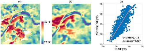
The LLST pattern extraction is demonstrated in Figure 3., taking LST maps in 2002 as an example. As shown in Figure 3, MTGP generated a smoother and more detailed surface than raw LST data and interpolated missing observations due to cloud contamination. Furthermore, the LLST pattern was produced by MTGP with superior accuracy. Exemplified by the raw MODIS LST and LLST on July 28th, 2007 (Figure 4), the resampled 1000-meter LLST is highly coherent to raw MODIS LST (R² = 0.937).

Figure 4. (a) Raw MODIS LST map on July 28th, 2007 at 1000-m resolution; (b) LLST extracted by MTGP at 500-m resolution; (c) The scattered plot of MODIS LST and resampled 1000-m LLST

The accuracy of LLST patterns in 2002, 2007, 2012, and 2017 are evaluated by the Root Mean Square Error (RMSE), Standard Deviation (STD), Correlation Coefficient (CC). As reported in Table 3, the RMSEs of the predicted LLST patterns are all within two STD from raw LST data, and the CC values higher than 0.93 indicates LLST patterns and raw LST data are highly coherent.

Table 3. Accuracy assessments of LLST patterns from 2002 to 2017

Date	RMSE	STD	Two STD	CC
2002/07/12	0.97	1.28	2.56	0.96
2007/07/28	1.03	0.85	1.70	0.93
2012/07/21	0.88	0.92	1.84	0.97
2017/07/20	1.19	1.13	2.26	0.94

4.2. Identification of local hotspots by GMM

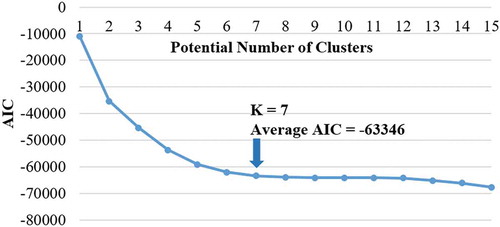
The spatial differentiation using GMM generally requires prior knowledge for specifying the clusters amount to be categorized into (ZZhao et al. 2016; Aghabozorgi, Shirkhorshidi, and Wah 2015). In this study, the cluster amount is defined using the Akaike Information Criterion (AIC), as shown in Figure 5. Because the AIC values of GMM clustering in 2002, 2007, 2012, and 2017 are very close. Thus, for better visualization, the average AIC values of four years are shown in Figure 5. When the number of the clusters is seven, AICs almost achieves the minimum value and is almost constant.

Figure 5. Determination of the optimal clusters for spatial clustering in GMM using average AIC value in four years

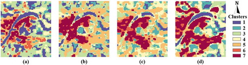
The spatial clusters in 2002, 2007, 2012, and 2017 are shown in Figure 6. The seventh cluster is defined as local LLST hotspots for the highest LLST values and MSSI values. Figure 6 shows that the local hotspots were expanding from the central downtown area of Wuhan to the surrounding suburban areas. The spatial extents of local hotspots in 2002, 2007, 2012, and 2017 are 217.03 km², 301.69 km², 363.16 km², and 532.82 km², respectively. According to the spatial clustering results of LLST patterns shown in Figure 5, the land cover types corresponding to the first and second clusters are rivers (the Yangtze River), lakes (the East Lake, the South Lake, and the Wu Lake), green spaces, etc. which are generally considered as “Urban Cool Island” (UCI) (Wang, Zhan, and Ouyang 2019; Rasul, Balzter, and Smith 2015). However, the seventh clusters are mainly the impervious surface in urban areas.

From 2002 to 2007, the local hotspots have expanded almost uniform in all directions and have shown prominent internal filling characteristics. From 2007 to 2012, the hotspots to significant expansion to the southeast. Specifically, the Optics Valley high-tech zone within Hongshan District and the surroundings become the newly emerged LLST hotspots. In 2017, a significant expansion of local hotspot, covering the Huashan new town, bordering area between Jiangxia District and Wuchang Area, Panlongcheng area, the North Hankou area, the Yangluo new town, has been witnessed in Wuhan.

Figure 6. The spatial differentiation of LLST patterns from 2002 to 2017. (a) 2002; (b) 2007; (c) 2012; (d) 2017

As the LLST and MSSI values of 7 clusters in four years reported in Table 4, the highest LLST and MSSI values are witnessed in seventh clusters in four years. Besides, the LLST values in seventh clusters show a slow linear growth from 2002 to 2017. The variations of MSSI values exhibit distinct characteristics. Specifically, the MSSI values of the first and second clusters gradually increased, while the MSSI value of the seventh cluster decreased significantly. Referring back to Section 3.2, MSSI value shall increase when the target surface bulges out from the surroundings and present noticeable isolation features (that is, the target surface presents island-like or cap-like features). The reason for the decrease of MSSI is the opposite. As shown in Figure 5, local LLST hotspots expanded with evident internal filling from 2002 to 2017. Thus, such variation leads to the decline of MSSI in seventh clusters (local hotspots). Similarly, as the hotspot has expanded, the first and second clusters shrunk and segregated. As a morphological perspective, such transformation resulted in a cup-like feature, i.e., a decline in MSSI value.

Table 4. LLST and MSSI values of 7 specific clusters

Cluster Number	LLST				MSSI
	2002	2007	2012	2017	2002	2007	2012	2017
1	25.68	26.01	26.32	26.59	–0.654	–0.683	–0.698	–0.712
2	27.84	28.34	27.91	27.83	–0.415	–0.475	–0.537	–0.561
3	28.11	29.65	28.36	28.77	–0.264	–0.231	–0.228	–0.225
4	29.93	30.74	30.12	30.84	0.207	0.227	0.182	0.187
5	30.35	31.61	32.54	33.91	0.492	0.553	0.402	0.343
6	32.06	32.94	33.79	34.63	0.721	0.718	0.615	0.521
7	33.18	33.87	35.63	36.82	0.872	0.811	0.709	0.696

4.3. Spatial and temporal dynamics of HSWMC

The spatial and temporal variations of HSWMC are calculated in 2002, 2007, 2012, and 2017 at the whole region scale, respectively. Qualitatively, the HSWMCs in Wuhan gradually to southeast direction overall. From 2002 to 2007, the HSWMC of mass shifted slightly to the northeast, and from 2007 to 2012, the HSWMCs of the group moved a considerable distance to the southeast. In 2017, it moved southeast to the East Lake. Quantitatively, the HSWMCs from 2002 to 2017 is located in Wuchang District within the geographical extent of ${30}^{\circ }{33}^{\prime }16{ }^{\prime \prime }\mathrm{N}-{30}^{\circ }{47}^{\prime }32{ }^{\prime \prime }\mathrm{N}$, ${114}^{\circ }{18}^{\prime }32{ }^{\prime \prime }\mathrm{E}-{114}^{\circ }{21}^{\prime }48{ }^{\prime \prime }\mathrm{E},$ as shown in Figure 7. The detailed information on HSWMCs’ moving trajectories during this period are reported in Table 5.

Figure 7. The spatial pattern of hotspots weighted mean centers (HSWMCs) from 2002 to 2017

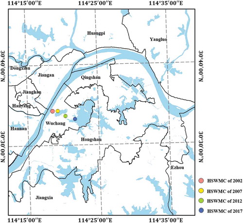
Table 5. LLST and MSSI values of 7 specific clusters

Period	Distance (m)	Direction	Moving rate (m/Year)
2002–2007	1254.24	North by East 83.56°	250.85
2007–2012	2096.07	South by East 71.84°	419.21
2012–2017	2360.59	South by East 76.75°	472.12

Quantitatively, the HSWMC in 2002 is located at ${30}^{\circ }{34}^{\prime }12{ }^{\prime \prime }\mathrm{N}$, ${114}^{\circ }{18}^{\prime }32{ }^{\prime \prime }\mathrm{E}$, and moved 1254.24 m northeast to ${30}^{\circ }{34}^{\prime }18{ }^{\prime \prime }\mathrm{N}$, ${114}^{\circ }{19}^{\prime }19{ }^{\prime \prime }\mathrm{E}$. Such movements can be resulted by the heating effect of Qingshan industrial park located northeast from the HSWMC in 2002. From 2007 to 2012, the movement distances increase to 2096.07 m, and the moving direction deflects to the south by east 71.84°. In 2017, the HSWMC moved southeast with an average annual movement rate of 472.12 m, and the distance increased about 300 m. The movements of HSWMCs from 2002 to 2017 demonstrate that local LLST hotspots within Wuhan expand in a southeast direction overall during this period. Specifically, the intensive expansions of local LLST hotspots mainly occurred in the southeast part of the study area, i.e., the Optics Valley high-tech zone, and the Huashan new town. Such local LLST hotspots are positively correlated to the IS expansion, as examined in our previous study conducted in Wuhan (Yang et al. 2019).

4.4. Orientation and dispersion analysis of local hotspots

To depict the spatial and temporal variations of orientations and expansion patterns of local hotspots within Wuhan, the weighted SDE is adopted in this study. The SDEs of local LLST hotspots within Wuhan are shown in Figure 8, and the detailed shape characteristics of SDEs from 2002 to 2017 are reported in Table 6.

Figure 8. Standard Deviation Eclipses (SDEs) of local LLST hotspots within Wuhan

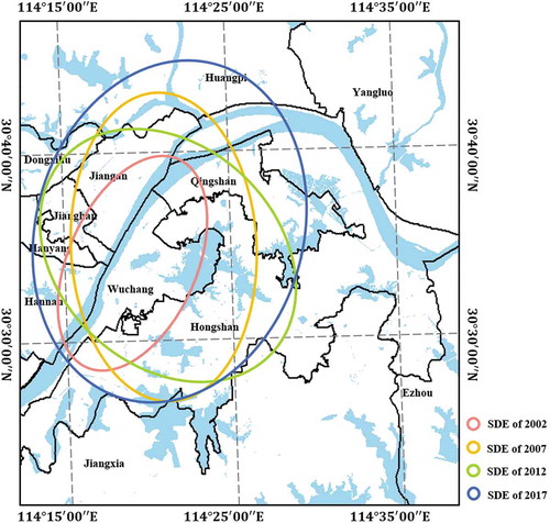
Table 6. Parameters of SDEs from 2002 to 2017

Year	Rotation Angle	Long Axis	Short Axis	Long/Short Ratio
2002	18.73°	13,835.44	8579.27	1.61
2007	177.19°	16,686.52	11,199.01	1.49
2012	141.12°	19,838.00	14,804.48	1.34
2017	9.02°	21,271.32	17,017.56	1.25

As shown in Figure 8, the orientations and directivity of local LLST hotspots varied with time dramatically. Specifically, the azimuths of SDEs clockwise increased from 18.73° in 2002 to 177.19° in 2007. After that, from 2012 to 2017, the azimuths anticlockwise decreased from 141.12° to 9.02°. This transformation of SDEs’ azimuths can be ascribed to the directional expansions of local LLST patterns in the suburban surroundings. Referring to Section 4.2, from 2002 to 2012, the growth of local hotspots mainly occurred in the southeast part of the study area (precisely, the Optics Valley high-tech zone and the surroundings). Such variations lead to the dramatic diversions of SDEs in this period. From 2012 to 2017, the intensive expansions of hotspots did not present obvious directivity, which brings about the circle-like SDE in 2017.

The dispersion degree of local LLST hotspots is measured by the long/short axis of the ratio of the short and long axis of SDE. As reported in Table 6, the decreasing rate from 2002 to 2017 reveals that the shape of the SDE is increasingly circular. Such a decrease of the long/short axis implicit that the dispersion degree of local LLST hotspots shows a significant increase. This variations of SDEs are reasonable from the perspective that the expansion of local hotspots by dramatical expansion of built-up areas within the study area from 2002 to 2017, which are consistent with the results in previous studies (Liu et al. 2018; Liu et al. 2019a; Shen et al. 2016).

4.5. Quantitative local warming effect of impervious surface

To further explore the latent impacts of IS on local LST anomalies, the associations between the composition and configuration characteristics of IS and summertime LLST patterns in Wuhan have been quantified using RF. The VIMs of composition and configuration features of IS are numerically revealed by %IncMSE as shown in Figure 9.

Figure 9. Variable Importance Measurements (VIMs) of landscape metrics in (a) 2002, (b) 2007, (c) 2012 and (d) 2017

According to the results demonstrated in Figure 9, the IS composition is generally responsible for local LLST patterns in Wuhan, and configuration characteristics of IS show diverse impacts on LST anomalies. As shown in Figure 9, the VIMs of CLASS_PLAND are the highest in 2002, 2007, 2012, and 2017. Such results reveal that the IS percent coverage is the most significant external forcing of local LST anomalies in Wuhan from 2002 to 2017. The VIMs of configuration metrics are consistent with the finds by Zhou et al. (2011) and Chen et al. (2014) that “configuration also matters.” In particular, CLASS_PD (mean %IncMSE equals to 23.88) and CLASS_AI (mean %IncMSE equals to 22.59) demonstrated the most significant impacts on the local thermal environment. Besides, CLASS_AREA_MN also shows remarkable importance in the explanation of local LST anomalies from 2002 to 2017. However, the IS shape characteristics (i.e., CLASS_SHAPE_MN and CLASS_SHAPE_STD) exerts negligible impacts on local LLST patterns (mean %IncMSEs equal to 6.32 and 6.17, respectively). Furthermore, contrary to the findings by Chen et al. (2014), edge metrics remarkably affect the LLST pattern in 2002 but do not have significant influences on local LST anomalies in Wuhan from 2007 to 2017. Such results can be explained by the evolution of IS patterns from 2002 through 2017 (Zhan, Yue, and Xiao 2018). From 1995 to 2005, the IS expansions in Wuhan were mainly composed of the low/medium-rise and high-density residential areas with significant edge diversity. In 2005–2015, the IS renewal in Wuhan was mainly an industrial zone and a considerable lot of high-rise and low/medium-density residential areas. Such a built-up area generally has regular shapes and edges (Zhan, Yue, and Xiao 2018; Huang et al. 2019).

5. Conclusions

This study presents a general framework for characterizing the spatial and temporal patterns and variations as well as spatiotemporal trajectories of local LST hotspots at a local scale. The local LST hotspots in Wuhan from 2002 to 2017 are extracted from LLST patterns generated by MTGP with the aid of morphological features quantified by MSSI using GMM clustering. The findings of this study can be summarized as:

1. During the specific period of 2002–2017, the spatial extents of local LST hotspots have been expanded significantly from 217.03 km² to 532.82 km².

2. The expansion of local hotspots in Wuhan mainly head to the southeast direction, and the dispersion degree of LLST hotspots generally increased from 2002 to 2017. Such findings are consistent with the IS expansion in Wuhan.

3. As the quantitative impacts of composition and configuration characteristics on local LLST anomalies demonstrate, the configuration characteristics are also responsible for the local LLST anomalies, especially the mean IS area, IS patches density, and aggregation degree of IS patches.

By focusing on the LLST spatial and temporal variations characterization, this study can promote the synergies between urban thermal environment studies and urban planning practices and can provide practical implications for decision making of urban expansion steering considering the underlying adverse effects by IS on the local thermal environment. The local LLST hotspots and its spatial and temporal variations are correlated to urban forms (Yang et al. 2018), urban functions (Liu et al. 2019b), and other land surface factors (Liu et al. 2019a; Shen et al. 2016), thus facilitating the implementation of UHI mitigation and adaptation strategies. Nevertheless, some considerations deserve further investigations in the following studies, such as the Annual Temperature Cycle (ATC) (Weng and Fu 2014a) and seasonal variation (Liu et al. 2019b) of LST and the underlying relationship between LST and landscapes.

Data availability statement

The raw land surface temperature data can be obtained from the Level 1 and Atmosphere Archive and Distribution System (LAADS, https://ladsweb.modaps.eosdis.nasa.gov/).

Additional information

Funding

This work is supported by the National Natural Science Foundation of China [grant numbers 51878515, 51378399, and 41331175].

Notes on contributors

Chen Yang

Chen Yang is a Ph.D. candidate in College of Urban and Environmental Sciences, Peking University. He received his master’s degree from School of Urban Design, Wuhan University in 2020. His research interests include thermal infrared remote sensing, quality development of remotely sensed image, climate change, and urban sustainability

Qingming Zhan

Qingming Zhan is currently a professor with School of Urban Design, Wuhan University. Prof. Zhan received his Ph.D. degree in geo-information science from Wageningen University - ITC, the Netherlands in 2003. His research interests include digital and smart cities, planning support systems, object-based analysis of remote sensing images, etc.

Sihang Gao

Sihang Gao is a graduate student at Wuhan University. His research interests include spatial statistics, urban planning, urban thermal environment.

Huimin Liu

Huimin Liu is a postdoc scholar of The Chinese University of Hong Kong under the supervision of Prof. Bo Huang. Her research interests include urban sustainability, environmental patterns and dynamics, health cities, climate change, and remote sensing.

References

- Aghabozorgi, S., A. S. Shirkhorshidi, and T. Y. Wah. 2015. “Time-series Clustering – A Decade Review.” Information Systems 53: 16–38. doi:10.1016/j.is.2015.04.007.
- Bonilla, E. V. 2008. “Multi-task Gaussian Process Prediction.” Advances in Neural Information Processing Systems 20: 153–160.
- Breiman, L. 2001. “Random Forests.” Machine Learning 45 (1): 5–32. doi:10.1023/A:1010933404324.
- Chen, A., L. Yao, R. Sun, and L. Chen. 2014. “How Many Metrics are Required to Identify the Effects of the Landscape Pattern on Land Surface Temperature?” Ecological Indicators 45: 424–433. doi:10.1016/j.ecolind.2014.05.002.
- Chen, Y.-C., H.-W. Chiu, Y.-F. Su, Y.-C. Wu, and K.-S. Cheng. 2017. “Does Urbanization Increase Diurnal Land Surface Temperature Variation? Evidence and Implications.” Landscape and Urban Planning 157: 247–258. doi:10.1016/j.landurbplan.2016.06.014.
- Dos Santos, A. R., F. S. De Oliveira, A. G. Da Silva, J. M. Gleriani, W. Gonçalves, G. L. Moreira, F. G. Silva, et al. 2017. “Spatial and Temporal Distribution of Urban Heat Islands”. Science of the Total Environment 605–606: 946–956. doi:10.1016/j.scitotenv.2017.05.275.
- Gong, P., X. Li, and W. Zhang. 2019. “40-Year (1978–2017) Human Settlement Changes in China Reflected by Impervious Surfaces from Satellite Remote Sensing.” Science Bulletin 64 (11): 756–763. doi:10.1016/j.scib.2019.04.024.
- Hao, P., Z. Niu, Y. Zhan, Y. Wu, L. Wang, and Y. Liu. 2016. “Spatiotemporal Changes of Urban Impervious Surface Area and Land Surface Temperature in Beijing from 1990 to 2014.” GIScience & Remote Sensing 53 (1): 63–84. doi:10.1080/15481603.2015.1095471.
- Huang, B., and J. Wang. 2020. “Big Spatial Data for Urban and Environmental Sustainability.” Geo-spatial Information Science 23 (2): 125–140. doi:10.1080/10095020.2020.1754138.
- Huang, Q., J. Huang, X. Yang, C. Fang, and Y. Liang. 2019. “Quantifying the Seasonal Contribution of Coupling Urban Land Use Types on Urban Heat Island Using Land Contribution Index: A Case Study in Wuhan, China.” Sustainable Cities and Society 44: 666–675. doi:10.1016/j.scs.2018.10.016.
- Koenderink, J. J., and A. J. van Doorn. 1992. “Surface Shape and Curvature Scales.” Image and Vision Computing 10 (8): 557–564. doi:10.1016/0262-8856(92)90076-F.
- Kuang, W., A. Liu, Y. Dou, G. Li, and D. Lu. 2019. “Examining the Impacts of Urbanization on Surface Radiation Using Landsat Imagery.” GIScience & Remote Sensing 56 (3): 462–484. doi:10.1080/15481603.2018.1508931.
- Kuang, W., Y. Liu, Y. Dou, W. Chi, G. Chen, C. Gao, T. Yang, J. Liu, and R. Zhang. 2015. “What are Hot and What are Not in an Urban Landscape: Quantifying and Explaining the Land Surface Temperature Pattern in Beijing, China.” Landscape Ecology 30 (2): 357–373. doi:10.1007/s10980-014-0128-6.
- Kuang, W., Z. Li, and R. Hamdi. 2020. “Comparison of Surface Radiation and Turbulent Heat Fluxes in Olympic Forest Park and on a Building Roof in Beijing, China.” Urban Climate 31: 100562. doi:10.1016/j.uclim.2019.100562.
- Li, H., Y. Zhou, X. Li, L. Meng, X. Wang, S. Wu, and S. Sodoudi. 2018. “A New Method to Quantify Surface Urban Heat Island Intensity.” Science of the Total Environment 624: 262–272. doi:10.1016/j.scitotenv.2017.11.360.
- Li, W., Q. Cao, K. Lang, and J. Wu. 2017. “Linking Potential Heat Source and Sink to Urban Heat Island: Heterogeneous Effects of Landscape Pattern on Land Surface Temperature.” Science of the Total Environment 586: 457–465. doi:10.1016/j.scitotenv.2017.01.191.
- Li, X., and P. Gong. 2016. “An “Exclusion-inclusion” Framework for Extracting Human Settlements in Rapidly Developing Regions of China from Landsat Images.” Remote Sensing of Environment 186: 286–296.
- Li, X., P. Gong, and L. Liang. 2015. “A 30-year (1984–2013) Record of Annual Urban Dynamics of Beijing City Derived from Landsat Data.” Remote Sensing of Environment 166: 78–90. doi:10.1016/j.rse.2015.06.007.
- Liu, H., B. Huang, and C. Yang. 2020. “Assessing the Coordination between Economic Growth and Urban Climate Change in China from 2000 to 2015.” Science of the Total Environment 732: 139283. doi:10.1016/j.scitotenv.2020.139283.
- Liu, H., Q. Zhan, C. Yang, and J. Wang. 2018. “Characterizing the Spatio-temporal Pattern of Land Surface Temperature through Time Series Clustering: Based on the Latent Pattern and Morphology.” Remote Sensing 10 (4): 654. doi:10.3390/rs10040654.
- Liu, H., Q. Zhan, C. Yang, and J. Wang. 2019b. “The Multi-timescale Temporal Patterns and Dynamics of Land Surface Temperature Using Ensemble Empirical Mode Decomposition.” Science of the Total Environment 652: 243–255. doi:10.1016/j.scitotenv.2018.10.252.
- Liu, H., Q. Zhan, S. Gao, and C. Yang. 2019a. “Seasonal Variation of the Spatially Non-stationary Association between Land Surface Temperature and Urban Landscape.” Remote Sensing 11 (9): 1016. doi:10.3390/rs11091016.
- Liu, Y., J. Peng, and Y. Wang. 2017. “Diversification of Land Surface Temperature Change under Urban Landscape Renewal: A Case Study in the Main City of Shenzhen, China.” Remote Sensing 9 (9): 919. doi:10.3390/rs9090919.
- Mcgarigal, K. 1995. FRAGSTATS: Spatial Pattern Analysis Program for Quantifying Landscape Structure. Vol. 351. US Department of Agriculture, Forest Service, Pacific Northwest Research Station.
- Nistor, -M.-M. 2019. “Vulnerability of Groundwater Resources under Climate Change in the Pannonian Basin.” Geo-spatial Information Science 22 (4): 345–358. doi:10.1080/10095020.2019.1613776.
- Oke, T. R. 1988. “Street Design and Urban Canopy Layer Climate.” Energy and Buildings 11 (1): 103–113. doi:10.1016/0378-7788(88)90026-6.
- Qiao, Z., N. Huang, X. Xu, Z. Sun, W. Chen, and J. Yang. 2019. “Spatio-temporal Pattern and Evolution of Urban Land Surface Thermal Landscape in Beijing Metropolitan Area between 2003 and 2017.” (in Chinese) Acta Geographica Sinica 74 (3): 475–489.
- Rajasekar, U., and Q. Weng. 2009. “Urban Heat Island Monitoring and Analysis Using A Non-parametric Model: A Case Study of Indianapolis.” ISPRS Journal of Photogrammetry and Remote Sensing 64 (1): 86–96. doi:10.1016/j.isprsjprs.2008.05.002.
- Rasul, A., H. Balzter, and C. Smith. 2015. “Spatial Variation of the Daytime Surface Urban Cool Island during the Dry Season in Erbil, Iraqi Kurdistan, from Landsat 8.” Urban Climate 14: 176–186. doi:10.1016/j.uclim.2015.09.001.
- Shao, Z., N. S. Sumari, A. Portnov, F. Ujoh, W. Musakwa, and P. J. Mandela. 2020. “Urban Sprawl and Its Impact on Sustainable Urban Development: A Combination of Remote Sensing and Social Media Data.” Geo-spatial Information Science 1–15. doi:10.1080/10095020.2020.1787800.
- Shen, H., L. Huang, L. Zhang, P. Wu, and C. Zeng. 2016. “Long-term and Fine-scale Satellite Monitoring of the Urban Heat Island Effect by the Fusion of Multi-temporal and Multi-sensor Remote Sensed Data: A 26-year Case Study of the City of Wuhan in China.” Remote Sensing of Environment 172: 109–125. doi:10.1016/j.rse.2015.11.005.
- Stewart, I. D., and T. R. Oke. 2012. “Local Climate Zones for Urban Temperature Studies.” Bulletin of the American Meteorological Society 93 (12): 1879–1900.
- Streutker, D. R. 2003. “Satellite-measured Growth of the Urban Heat Island of Houston, Texas.” Remote Sensing of Environment 85 (3): 282–289. doi:10.1016/S0034-4257(03)00007-5.
- Tomlinson, C. J., L. Chapman, J. E. Thornes, and C. J. Baker. 2012. “Derivation of Birmingham’s Summer Surface Urban Heat Island from MODIS Satellite Images.” International Journal of Climatology 32 (2): 214–224. doi:10.1002/joc.2261.
- Trinder, J., and Q. Liu. 2020. “Assessing Environmental Impacts of Urban Growth Using Remote Sensing.” Geo-spatial Information Science 23 (1): 20–39. doi:10.1080/10095020.2019.1710438.
- Wan, Z. 2008. “New Refinements and Validation of the MODIS Land-Surface Temperature/Emissivity Products.” Remote Sensing of Environment 112 (1): 59–74. doi:10.1016/j.rse.2006.06.026.
- Wan, Z. 2014. “New Refinements and Validation of the Collection-6 MODIS Land-surface Temperature/emissivity Product.” Remote Sensing of Environment 140: 36–45. doi:10.1016/j.rse.2013.08.027.
- Wang, J., Q. Zhan, and H. Guo. 2016b. “The Morphology, Dynamics and Potential Hotspots of Land Surface Temperature at a Local Scale in Urban Areas.” Remote Sensing 8 (1): 18. doi:10.3390/rs8010018.
- Wang, J., Q. Zhan, H. Guo, and Z. Jin. 2016a. “Characterizing the Spatial Dynamics of Land Surface Temperature–impervious Surface Fraction Relationship.” International Journal of Applied Earth Observation and Geoinformation 45: 55–65. doi:10.1016/j.jag.2015.11.006.
- Wang, Y., Q. Zhan, and W. Ouyang. 2019. “How to Quantify the Relationship between Spatial Distribution of Urban Waterbodies and Land Surface Temperature?” Science of the Total Environment 671: 1–9. doi:10.1016/j.scitotenv.2019.03.377.
- Warren Liao, T. 2005. “Clustering of Time Series Data—a Survey.” Pattern Recognition 38 (11): 1857–1874. doi:10.1016/j.patcog.2005.01.025.
- Weng, Q., M. K. Firozjaei, A. Sedighi, M. Kiavarz, and S. K. Alavipanah. 2019. “Statistical Analysis of Surface Urban Heat Island Intensity Variations: A Case Study of Babol City, Iran.” GIScience & Remote Sensing 56 (4): 576–604. doi:10.1080/15481603.2018.1548080.
- Weng, Q., and P. Fu. 2014a. “Modeling Annual Parameters of Clear-sky Land Surface Temperature Variations and Evaluating the Impact of Cloud Cover Using Time Series of Landsat TIR Data.” Remote Sensing of Environment 140: 267–278. doi:10.1016/j.rse.2013.09.002.
- Weng, Q., and P. Fu. 2014b. “Modeling Diurnal Land Temperature Cycles over Los Angeles Using Downscaled GOES Imagery.” ISPRS Journal of Photogrammetry and Remote Sensing 97: 78–88. doi:10.1016/j.isprsjprs.2014.08.009.
- Xu, J., Y. Zhao, K. Zhong, F. Zhang, X. Liu, and C. Sun. 2018. “Measuring Spatio-temporal Dynamics of Impervious Surface in Guangzhou, China, from 1988 to 2015, Using Time-series Landsat Imagery.” Science of the Total Environment 627: 264–281. doi:10.1016/j.scitotenv.2018.01.155.
- Yang, C., Q. Zhan, J. Zhang, H. Liu, and Z. Fan. 2018a. “Quantifying the Relationship between Natural and Socioeconomic Factors and with Fine Particulate Matter (PM2.5) Pollution by Integrating Remote Sensing and Geospatial Big Data.” The International Archives of the Photogrammetry, Remote Sensing and Spatial Information Sciences XLII-3/W5: 77–82. doi:10.5194/isprs-archives-XLII-3-W5-77-2018.
- Yang, C., Q. Zhan, S. Gao, and H. Liu. 2019a. “How Do the Multi-temporal Centroid Trajectories of Urban Heat Island Correspond to Impervious Surface Changes: A Case Study in Wuhan, China.” International Journal of Environmental Research and Public Health 16 (20): 3865. doi:10.3390/ijerph16203865.
- Yang, C., Q. Zhan, Y. Lv, and H. Liu. 2019b. “Downscaling Land Surface Temperature Using Multiscale Geographically Weighted Regression over Heterogeneous Landscapes in Wuhan, China.” IEEE Journal of Selected Topics in Applied Earth Observations and Remote Sensing 12 (12): 5213–5222. doi:10.1109/JSTARS.2019.2955551.
- Yang, C., Q. Zhan, Y. Xiao, and H. Liu. 2020. “Identifying the Driving Factors of Population Exposure to Fine Particulate Matter (PM2.5) In Wuhan, China.” The International Archives of the Photogrammetry, Remote Sensing and Spatial Information Sciences V-3-2020: 355–361. doi:10.5194/isprs-annals-V-3-2020-355-2020.
- Yang, J., J. Su, J. C. Jin, X. Li, and Q. Ge. 2018b. “The Impact of Spatial Form of Urban Architecture on the Urban Thermal Environment: A Case Study of the Zhongshan District, Dalian, China.” IEEE Journal of Selected Topics in Applied Earth Observations and Remote Sensing 11 (8): 2709–2716. doi:10.1109/JSTARS.2018.2808469.
- Yang, J., P. Gong, R. Fu, M. Zhang, J. Chen, S. Liang, B. Xu, J. Shi, and R. Dickinson. 2013. “The Role of Satellite Remote Sensing in Climate Change Studies.” Nature Climate Change 3: 1001. doi:10.1038/nclimate2033.
- Zhan, Q., Y. Yue, and Y. Xiao. 2018. “Evolution of Built-up Area Expansion and Verification of Planning Implementation in Wuhan, City.” Planning Review 42: 63–71.
- Zhang, D., X. Liu, X. Wu, Y. Yao, X. Wu, and Y. Chen. 2019. “Multiple Intra-urban Land Use Simulations and Driving Factors Analysis: A Case Study in Huicheng, China.” GIScience & Remote Sensing 56 (2): 282–308.
- Zhao, B., Y. Zhong, A. Ma, and L. Zhang. 2016. “A Spatial Gaussian Mixture Model for Optical Remote Sensing Image Clustering.” IEEE Journal of Selected Topics in Applied Earth Observations and Remote Sensing 9 (12): 5748–5759. doi:10.1109/JSTARS.2016.2546918.
- Zhou, D., J. Xiao, S. Bonafoni, C. Berger, K. Deilami, Y. Zhou, S. Frolking, R. Yao, Z. Qiao, and A. J. Sobrino. 2018. “Satellite Remote Sensing of Surface Urban Heat Islands: Progress, Challenges, and Perspectives.” Remote Sensing 11 (1): 48. doi:10.3390/rs11010048.
- Zhou, J., Y. Chen, J. Wang, and W. Zhan. 2011a. “Maximum Nighttime Urban Heat Island (UHI) Intensity Simulation by Integrating Remotely Sensed Data and Meteorological Observations.” IEEE Journal of Selected Topics in Applied Earth Observations and Remote Sensing 4 (1): 138–146. doi:10.1109/JSTARS.2010.2070871.
- Zhou, W., G. Huang, and M. L. Cadenasso. 2011b. “Does Spatial Configuration Matter? Understanding the Effects of Land Cover Pattern on Land Surface Temperature in Urban Landscapes.” Landscape and Urban Planning 102 (1): 54–63. doi:10.1016/j.landurbplan.2011.03.009.