Advances in spaceborne hyperspectral remote sensing in China

ABSTRACT

With the maturation of satellite technology, Hyperspectral Remote Sensing (HRS) platforms have developed from the initial ground-based and airborne platforms into spaceborne platforms, which greatly promotes the civil application of HRS imagery in the fields of agriculture, forestry, and environmental monitoring. China is playing an important role in this evolution, especially in recent years, with the successful launch and operation of a series of civil hyperspectral spacecraft and satellites, including the Shenzhou-3 spacecraft, the Gaofen-5 satellite, the SPARK satellite, the Zhuhai-1 satellite network for environmental and resources monitoring, the FengYun series of satellites for meteorological observation, and the Chang’E series of spacecraft for planetary exploration. The Chinese spaceborne HRS platforms have various new characteristics, such as the wide swath width, high spatial resolution, wide spectral range, hyperspectral satellite networks, and microsatellites. This paper focuses on the recent progress in Chinese spaceborne HRS, from the aspects of the typical satellite systems, the data processing, and the applications. In addition, the future development trends of HRS in China are also discussed and analyzed.

KEYWORDS:

• Hyperspectral remote sensing
• spaceborne HRS
• hyperspectral image processing and remote sensing applications

1. Introduction

Hyperspectral imaging, which is also called imaging spectrometry, possesses the dual advantages of spectroscopy and optical imaging, i.e., collecting abundant spectral characteristics of targets across the full spectrum, in addition to two-dimensional Dimensional (2-D) spatial images (Goetz et al. 1985). Following the development of hyperspectral imaging technology, it has aroused attention from scholars of both academic and industrial circles, and has been a research hotspot around the world (Li et al. 2016). In the early days, Hyperspectral Remote Sensing (HRS) was primarily utilized to identify targets against other backgrounds for military investigation. Nowadays, HRS has exhibited great potential in many application fields, e.g., environmental monitoring (Govender, Chetty, and Bulcock 2007; Adam, Mutanga, and Rugege 2010), mineralogy (Kruse, Boardman, and Huntington 2003; Galvão et al. 2008), astronomy (Hege et al. 2004), archeology (Liang 2012), medical diagnosis (Lu and Fei 2014), and food safety (Feng and Sun 2012; Khan et al. 2018), since it can provide both spatial features and invisible spectral features for the fine identification of materials.

The breakthrough in hyperspectral imaging originated from the Jet Propulsion Laboratory (JPL) in the 1980s (Goetz 2009), where the Airborne Imaging Spectrometer (AIS) was developed in 1983 (Vane, Goetz, and Wellman 1984) and the Airborne Visible/Infrared Imaging Spectrometer (AVIRIS) was developed in 1987 (Green et al. 1998) for remote sensing of the Earth. Hyperspectral imaging was first applied to airborne remote sensing, and a series of airborne HRS systems have now been developed around the world, such as AVIRIS, the Compact Airborne Spectrographic Imager (CASI) (Babey and Anger 1989), the Hyperspectral Digital Imagery Collection Experiment (HYDICE) (Rickard et al. 1993), and the Hyperspectral Mapper (HyMap) (Cocks et al. 1998). The research into HRS in China also originated from airborne remote sensing in the 1980s. Subsequently, several high-quality hyperspectral imagers, including the Pushbroom Hyperspectral Imager (PHI), the Modular Airborne Imaging Spectrometer (MAIS), and the Operational Modular Imaging Spectrometer (OMIS), were designed for the purposes of natural resource exploration during the 1990s. With the continuing development of hyperspectral sensors, hyperspectral image processing has become a hot research field in remote sensing.

The appearance of spaceborne HRS systems came slightly after the airborne HRS systems. Spaceborne HRS also originated at NASA, where the Hyperion imaging spectrometer onboard the Earth Observing-1 (EO-1) satellite (Ungar et al. 2003) was launched in 2000. This satellite successfully operated for more than 15 years, providing a large number of HRS images for scientific research, and starting the new era of HRS observation of the Earth at a global scale. Hyperion data contain 220 spectral channels covering a spectral range of 0.4–2.5 μm, and the spatial resolution and swath width are 30 m and 7.7 km, respectively, at an orbit altitude of 705 km. Currently, Hyperion is still one of the most important sources of spaceborne HRS data. The Compact High-Resolution Imaging Spectrometer (CHRIS) onboard the Project for On-Board Autonomy (PROBA) satellite was launched in 2001 by the European Space Agency (ESA). CHRIS data contain 62 spectral bands covering a spectral range of 0.4–1.05 μm, and the spatial resolution and the swath width are 34 m and 14 km, respectively, at an orbit altitude of 556 km. However, compared with the abundant airborne HRS systems, there is only a limited number of hyperspectral satellites in orbit for civil use. In addition, due to the limited hyperspectral detector array sizes, spaceborne HRS systems generally feature a low spatial resolution and narrow swath width.

In recent decades, China has played an important role in the development of the civil spaceborne HRS systems, with a series of hyperspectral satellites being successfully designed and launched for various applications. Figure 1 illustrates the development history of the spaceborne HRS sensors of China, including the hyperspectral imagers onboard satellites, lunar probes, and manned space experimental platforms. The detailed parameters of these sensors are summarized in Table 1. The Chinese Moderate Resolution Imaging Spectroradiometer (CMODIS) onboard the Shenzhou-3 (SZ-3) spacecraft was the first spaceborne hyperspectral imager developed in China, which was followed by a series of hyperspectral satellites for the observation of the Earth’s surface, including Huanjing-1A (HJ-1A), Tiangong-1 (TG-1), SPARK, Gaofen-5 (GF-5), and Zhuhai-1. GF-5 is the world’s first hyperspectral satellite covering the full spectral range, realizing simultaneous observation of the land and atmosphere. The Zhuhai-1 mission is the first Chinese commercial microsatellite constellation and is made up of 10 Orbita Hyperspectral Satellites (OHSs). This satellite network greatly improves the temporal resolution of spaceborne HRS. Hyperspectral imagers are also used for atmospheric monitoring, e.g., the Medium-Resolution Spectral Imager onboard the FY-3 series of satellites successively launched from 2008 to 2017. In addition to Earth observation, hyperspectral imagers are also used in the Chinese Lunar Exploration Program (CLEP), e.g., the Sagnac-based Imaging Interferometer (IIM) used in the Chang’E series of satellites and the Visible and Near-Infrared Imaging Spectrometer (VNIS) used in the Yutu lunar rover.

Figure 1. The development history of the spaceborne HRS sensors in China

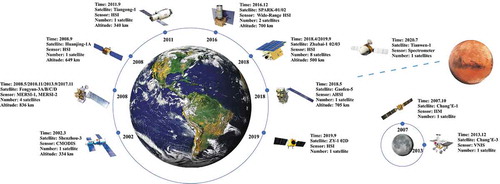
Table 1. Specifications of the chinese spaceborne HRS sensors

Sensor	Year	Altitude (km)	Spectral range (μm)	Spectral res. (nm)	Bands	Spatial res. (m)	Swath width (km)	Satellite net
SZ-3 CMODIS	2002	334	0.4–12.5	20–1000	34	400–500	650–700	No
Chang’E-1 IIM	2007	–	0.48–0.96	325.5 cm^−1	32	200	25.6	No
Chang’E-3 VNIS	2016	–	0.45–2.4	2–12	400	–	–	No
FY-3 MERSI-1	2008	836	0.4–12.5	20–1000	20	250/1000	2048	Yes
FY-3 MERSI-2	2017	836	0.4–12.5	20–1000	25	250/1000	2048	Yes
HJ-1A HSI	2008	649	0.45–0.95	5	115	100	50	Yes
TG-1 HSI	2011	340	0.4–2.5	10/20	128	10/20	10	No
SPARK HSI	2016	700	0.41–1.11	4.5	160	50	100	Yes
GF-5 AHSI	2018	705	0.4–2.5	5/10	330	30	60	No
OHS HSI	2018	500	0.41–1.11	2.5	32	10	150	Yes
ZY-1 02D HSI	2019	–	0.4–2.5	10/20	166	30	60	Yes
Tianwen-1 Spectrometer	2020	–	0.45–3.4	10/12/25	–	–	–	No

The growth in spaceborne HRS in China can be attributed to the microsatellite technology and the maturation of hyperspectral imaging technology. As shown in Table 1, the swath width of spaceborne HRS has gradually improved to meet the need for large-scale observation and has reached 150 km in the Zhuhai-1 mission with a 10-m spatial resolution. In addition, HRS satellite constellations are also a growing trend in China, as they can greatly enhance the temporal resolution of HRS, owing to the joint observation.

This paper focuses on the recent progress in spaceborne HRS in China, including the typical spaceborne HRS systems and the corresponding hyperspectral image processing and applications. The rest of this paper consists of four sections discussing spaceborne HRS in China in detail. Section 2 describes the spaceborne HRS systems for civil use in China. Section 3 focuses on the related data processing methods, such as preprocessing, classification, detection, retrieval, and data fusion. Section 4 summarizes the typical application cases of Chinese spaceborne hyperspectral systems. The developing trends and drawbacks of spaceborne HRS are discussed and analyzed in Section 5.

2. Chines spaceborne hyperspectral missions

This section is aimed at analyzing the characteristics of the Chinese spaceborne HRS systems in detail, including SZ-3 CMODIS, the FY-3 series, HJ-1A, TG-1, SPARK, GF-5, and Zhuhai-1.

2.1. SZ-3 CMODIS

The first spaceborne hyperspectral/multispectral sensor developed in China was the Chinese Moderate Resolution Imaging Spectroradiometer (CMODIS) (Chen et al. 2003) onboard the Shenzhou-3 (SZ-3) spacecraft launched by the China National Space Agency (CNSA) on 25 March 2002. Along with the manned space flight experiment, a space application experiment project was carried out when the SZ-3 spacecraft was on-orbit. The CMODIS sensor was designed for research into the ocean, land, and atmosphere, and it conducted continuous remote sensing observations of the Earth during the mission. The detailed parameters of the CMODIS sensor are summarized in Table 2. Nearly 400 orbits were completed in this mission, until the SZ-3 spacecraft ended its mission on 1 April 2002. Compared with the conventional multispectral remote sensing data available at that time, such as Landsat Thematic Mapper (TM), SPOT, and Advanced Very-High-Resolution Radiometer (AVHRR) data, the spectral resolution of the CMODIS sensor represented a great improvement. The CMODIS sensor was the first Chinese spaceborne hyperspectral imager, and it was also the first spaceborne hyperspectral imager in the world with continuous spectral bands in both the visible and near-infrared (VNIR), shortwave infrared (SWIR), and thermal infrared (TIR) spectral ranges.

Table 2. Main specifications of the CMODIS sensor

Specifications	VIS	NIR	SWIR	TIR
Wavelength (μm)	0.40–0.80	0.82–1.02	2.15–2.25	8.4–8.9	10.3–12.5
Spectral bands	20	10	1	1	2
Spectral resolution (nm)	20	20	100	500	1000
SNR	≥1000	≥1000	≥300	≤0.25 K @300 K	≤0.25 K @300 K
Swath width	650–700 km
Spatial resolution	400–500 m @ 334 ± 5 km orbit height

2.2. Chang’E series

The moon is the only natural satellite and the nearest celestial body to the Earth, with a 384,400 km average distance. Since the Luna 1 lunar probe was launched in the 1950s, more than 100 lunar missions have been conducted around the world. Relevant researchers have found more than 100 kinds of minerals on the lunar surface, many of which are rare minerals on Earth, which represent important supplements and reserves to the Earth’s natural resources. The lunar exploration mission in China is called the Chinese Lunar Exploration Program (CLEP). The CLEP is characterized by three distinct stages, i.e., “orbiting around”, “landing on”, and “returning from” the moon. To date, China has launched four lunar probes, i.e., Chang’E-1, Chang’E-2, Chang’E-3, and Chang’E-4, where Chang’E-2 and Chang’E-4 are the backups to Chang’E-1 and Chang’E-3, respectively.

The Chang’E-1 probe, launched in October 2007, was mainly aimed at implementing a circumlunar mission and obtaining global lunar images. Eight sets of instruments were carried on Chang’E-1, including a hyperspectral imager and the Sagnac-based Imaging Interferometer (IIM) (Marzi, Marinoni, and Gamba 2019), which was designed to analyze the chemical composition of minerals on the lunar surface through the observation of nearly 84% of the lunar surface from 70°N to 70°S. The main specifications of the IIM are listed in Table 3. The Chang’E-1 probe ended its mission in March 2009 after 495 days of observation on-orbit. From the observed hyperspectral data of Chang’E-1 IIM, high spatial resolution maps of lunar iron and titanium content have been generated.

Table 3. Main specifications of the chang’e sensors

Specifications	IIM	VNIS
Wavelength (μm)	0.48–0.96	0.45–0.95	0.9–2.4
Spectral bands	32	400
Spectral resolution	7.62 nm/29 nm	2–7 nm	3–12 nm
Digitization	12 bit	10 bit	16 bit
Pixel number	256 × 256	256 × 256	1
Swath width	25.6 km	–
Spatial resolution	200 m	–

Table 4. Main specifications of the MERSI-1 and MERSI-2 sensors

Specifications	MERSI-1		MERSI-2
	VNIR	TIR	VNIR	MIR	TIR
Wavelength (μm)	0.4–2.1	10–12.5	0.4–2.1	3.7–4.1	7.0–12.5
Spectral bands	19	1	19	2	4
Spectral resolution (nm)	20/50	2500	20–50	155–180	300–1000
Digitization	12 bit		12 bit
Pixel number	8192/2048		8192/2048
Swath width	2048 km		2048 km
Spatial resolution	250/1000 m		250/1000 m

The Chang’E-3 probe realized the first lunar soft landing of the CLEP, where the Yutu lunar rover was used to conduct surveys on the lunar surface. The VNIS sensor (Xiao et al. 2015) onboard the Yutu rover covered the 450–950 nm and 900–2400 nm spectral ranges. The default spectral sampling interval was 5 nm, with a total number of 400 spectral bands. The main specifications of the VNIS sensor are listed in Table 3. During the operation of the Yutu rover, hyperspectral images and spectral reflectance curves of the lunar soil in the region of Mare Imbrium were obtained. The Yutu rover operated for 972 days, and stopped operation on 31 July 2016. The Chang’E-1 IIM and Chang’E-3 VNIS data are available from http://moon.bao.ac.cn/index.jsp.

2.3. FY-3 series

To meet the needs of weather forecasting, environmental monitoring and climate prediction, the FengYun 3 (FY-3) series of satellites were launched from 27 May 2008 (http://fy4.nsmc.org.cn/nsmc/en/satellite/FY3.html). As the second generation of Chinese polar-orbit meteorological satellites, the FY-3 satellites are not affected by weather conditions and realize all-time and all-weather global observation from a near-polar solar-synchronous orbit at an average orbit altitude of 836 km, with an orbit inclination of 98.753°. To date, the FY-3A, FY-3B, FY-3C, FY-3D, and FY-3E satellites have been successfully launched, while the FY-3A satellite stopped operating in March 2018.

The FY-3A, FY-3B, and FY-3C satellites carry the Medium-Resolution Spectral Imager 1 (MERSI-1), which consists of 19 VNIR (0.4–2.1 μm) channels and a TIR channel (10–12.5 μm). In contrast, FY-3D and FY-3E are equipped with the MERSI-2 sensor, which integrates the function of the MERSI-1 sensor and the Visible and Infrared Radiometer (VIRR) instruments of the previous FY-3 satellites. The MERSI-2 sensor provides 25 spectral channels in the spectral range of 0.4–12.5 μm, and is the world’s first imaging instrument that can acquire infrared split-window data with a 250-m resolution. The FY-3 satellites can obtain 250-m resolution true-color images every day, without gaps, and can also obtain high-precision quantitative inversion parameters, such as atmospheric, cloud, aerosol, and water vapor data. As such, the FY-3 satellites provide environmental monitoring data for China. The major technical specifications of the MERSI-1 and MERSI-2 sensors are listed in Table 4.

FY-3A/B/C/D/E have formed a satellite network to implement joint Earth observation, greatly shortening the update interval for the observed data. MERSI-1 and MERSI-2 are capable of repeating observations of the same area every 5.5 days. Owing to the global observation ability, the MERSI-1 and MERSI-2 sensors can be used to: (1) provide datasets for the research into global climate change; (2) monitor large-scale natural disasters and the surface ecological environment; and (3) provide weather information for various professional activities, such as aviation, navigation, etc., in any area around the world. The FY-3 data are available from http://satellite.nsmc.org.cn/PortalSite/Default.aspx.

2.4. HJ-1A HSI

To realize large-scale, all-weather, and all-day dynamic monitoring of ecological damage and environmental pollution, China has developed the Huanjing-1 (HJ-1) satellite system, which is composed of two optical satellites, i.e., HJ-1A and HJ-1B, and a radar satellite, HJ-1 C (http://www.mee.gov.cn/home/ztbd/rdzl/wxyg/hjwx/201210/t20121010_237312.shtml). The HJ-1A satellite, which was launched on 6 September 2008, carries a hyperspectral imager which features 115 spectral bands covering the spectral range of 0.45–0.95 μm (Liao, Zhang, and Bao 2012). The major specifications of the HJ-1A Hyperspectral Imager (HSI) are listed in Table 5. In a solar-synchronous orbit, the HJ-1A HSI can revisit the same area on the Earth every 4 days. The orbit altitude of the HJ-1A satellite is 649.093 km, and the orbit inclination is 97.9486°.

Table 5. Main specifications of the HJ-1A HSI sensor

Specifications	HJ-1A HSI
Wavelength	0.45–0.95 μm
Spectral bands	110–128
Spectral resolution	5 nm
Spatial resolution	100 m
Swath width	50 km
Orbit altitude	649 km
Orbit inclination	97.9486°

HJ-1A and HJ-1B form a satellite network that circles the Earth in the same orbital plane to form complementary observations. Repeated observations can be made every day in most areas of China, which will greatly alleviate the shortage of Earth observation data for China and improve the ability to monitor environmental and ecological changes, as well as natural disasters. HJ-1A hyperspectral data have been applied in water and agricultural applications, such as the estimation of chlorophyll concentration in water and crop phenology mapping. The HJ-1A HSI data are available from http://www.chinageoss.cn/dsp/home/index.jsp.

2.5. TG-1 HSI

The Tiangong-1 (TG-1) space module was China’s first self-developed manned spaceborne experimental platform, which was launched on 29 September 2011. During this mission, the TG-1 spaceborne module supported environmental monitoring experiments. The hyperspectral imager onboard TG-1 was the most advanced space hyperspectral imager in China at this time, and was developed by the Shanghai Institute of Technical Physics (SITP) and the Changchun Institute of Optics, Fine Mechanics and Physics (CIOMP). The major technical specifications of the TG-1 HSI are listed in Table 6 (Lv et al. 2015). The TG-1 HSI provided 64 bands covering the VNIR spectral range (0.4–1.0 μm) and 64 bands covering the SWIR spectral range (1.0–2.5 μm). Most of the specifications of the TG-1 HSI approached or even exceeded those of EO-1 Hyperion, and for the swath width in particular, the TG-1 HSI exhibited obvious superiority. The TG-1 HSI was an important supplementary source of satellite hyperspectral data to the EO-1 Hyperion sensor, which was the only on-orbit spaceborne hyperspectral imager at the time of the launch of TG-1. The TG-1 HSI was designed mainly for scientific research in space and land-cover applications. To date, TG-1 HSI hyperspectral data have been applied in forest fire prevention, oil and gas exploration, hydro-ecological monitoring, and geological surveying. The TG-1 space module officially terminated the data service and ended its historic mission on 16 March 2016. The TG-1 HSI data are available from http://www.msadc.cn/sy/.

Table 6. Main specifications of the TG-1 HSIsensor compared to EO-1 hyperion

Specifications	TG-1 HSI		EO-1 Hyperion
	VNIR	SWIR	VNIR	SWIR
Wavelength (μm)	0.4–1.0	1.0–2.5	0.4–1.0	0.9–2.5
Spectral bands	64	64	60	160
Spatial resolution (m)	10	20	30	30
IFOV (°)	0.025	0.05	0.043
Swath width (km)	10		7.7
Orbit altitude (km)	340		705

IFOV = instantaneous field of view.

2.6. SPARK wide-range HSI

The wide-swath hyperspectral imaging microsatellites known as SPARK-01 and SPARK-02 were launched via the TanSat satellite on 22 December 2016. As microsatellites, the total weight of the SPARK satellite system is only 47 kg, and the wide-range hyperspectral imager onboard weighs only 10 kg. The major parameters of the SPARK wide-swath hyperspectral imaging system are listed in Table 7 (https://www.myorbita.net/). SPARK features 160 spectral bands within the spectral range of 400–1000 nm. It is noteworthy that the swath width of the SPARK HSI reaches 100 km at an orbit altitude of 700 km, which is more than 10 times the swath width of EO-1 (7.65 km). Furthermore, the swath width can reach 200 km through the cooperation of SPARK-01 and SPARK-02. With such a large swath width, the SPARK wide-range HSI can be used for rapid global data acquisition and dynamic monitoring of the environment. Through the observations of the SPARK satellite network, an area on the Earth’s surface of 2500 × 6000 km can be covered each day, obtaining more than 400 Gbit of hyperspectral data. The SPARK wide-range HSI can cover the whole of China within a month, and the observed data can be applied in the applications of agricultural prediction, pest and disease monitoring, environmental protection, and disaster monitoring.

Table 7. Main specifications of the SPARK wide-range HSI sensor

Specifications	SPARK wide-range HSI
Wavelength	0.4–1.0 μm
Spectral bands	160
Spectral resolution	4.5 nm
Spatial resolution	50 m
Swath width	100 km
Weight	47 kg
Orbit altitude	700 km

2.7. GF-5 AHSI

The Gaofen-5 (GF-5) satellite, which was launched on 9 May 2018, is a part of the China High-resolution Earth Observation System (CHEOS) of the China National Space Administration. Developed by the Shanghai Academy of Spaceflight Technology, GF-5 carries six instruments with a designed lifespan of 8 years, including VNIR and SWIR hyperspectral sensors, a greenhouse gas detector, a spectral imager, a differential absorption spectrometer, an atmospheric environment infrared detector, and a multi-angle polarization detector. It is noteworthy that GF-5 is the world’s first hyperspectral satellite covering the full spectral range, allowing it to realize comprehensive observation of the land and atmosphere.

The major parameters of the Advanced Hyper Spectral Imager (AHSI) onboard the GF-5 satellite are listed in Table 8 (Liu et al. 2019b). The GF-5 satellite orbits the Earth in a solar-synchronous orbit at an orbit altitude of 705 km, with a 30 m spatial resolution and a 60-km swath width. As a VNIR and SWIR hyperspectral imager, the AHSI instrument covers 330 spectral bands in the spectral range of 0.4–2.5 μm (2019b). The AHSI instrument cooperates with the multispectral imager, forming joint observation, and can revisit China’s territory and coastal areas every 5 days. The AHSI is the world’s first spaceborne hyperspectral imager which simultaneously considers both a wide swath width and a wide spectral range, which shortens the revisit time and promotes the observation scale.

Table 8. Main specifications of the GF-5 AHSI sensor

Specifications	AHSI
	VNIR	SWIR
Wavelength	0.4–1.0	1.0–2.5
Spectral resolution	5 nm	10 nm
Spectral bands	150	180
Swath width	60 km
Spatial resolution	30 m
Orbit altitude	705 km

2.8. OHS HSI

The Zhuhai-1 mission was the first commercial microsatellite constellation in China, and was designed by the Zhuhai Orbita Control Engineering Ltd. (https://www.myorbita.net/). The Zhuhai-1 mission consists of 34 microsatellites, including 12 video satellites, two high spatial resolution satellites, two radar satellites, eight infrared satellites, and 10 hyperspectral satellites. To date, there have been three batches of satellites launched, including five video satellites and eight hyperspectral satellites, which were launched on 15 June 2017, 26 April 2018, and 19 September 2019. Zhuhai-1 exhibits the properties of high spatial, spectral, and temporal resolutions.

The Orbita Hyperspectral Satellites (OHSs) carry the same type of hyperspectral imager, which features 256 spectral bands in the spectral range of 0.4–1.0 μm (https://www.myorbita.net/). The major technical specifications of the OHS HSI sensor are listed in Table 9. It is worth mentioning that the number of spectral bands of OHS is user-programmable. The number of spectral bands is adjustable according to the user requirements, allowing the user to select 32 bands from a total of 256 bands. The swath width and the spatial resolution of the OHSs are 150 km and 10 m, respectively, at an orbit altitude of 500 km, in a solar-synchronous orbit with an orbit inclination of 98°. The eight OHSs have already formed a satellite network for Earth observation. When 10 hyperspectral satellites are in orbit, the Earth-observing capability will be further improved. Joint observation by the network of 10 satellites could cover the Earth every 2 days and 182 times a year. As commercial hyperspectral satellites, the Zhuhai-1 satellites will greatly enrich the spaceborne hyperspectral data resources and will serve for scientific research and industrial applications. The OHS HSI data are available from https://www.obtdata.com/#/dataExpress.

Table 9. Main specifications of the OHS HSI sensor

Specifications	OHS HSI
Wavelength	0.4–1.1 μm
Spectral bands	32(256)
Spectral resolution (nm)	2.5
Spatial resolution (m)	10
Swath width (km)	150
SNR	≥300
Orbit parameters	Altitude: 500 km Inclination: 98°

2.9. ZY-1 02D HSI

ZY-1 02D satellite (5-m optical satellite) was launched on 12 September 2019, which is a medium-resolution remote sensing operational satellite under the auspices of the Ministry of Natural Resources. ZY-1 02D is a successor of ZY-1 02 C, which was mainly designed for high spectral resolution and medium spatial resolution, serving the tasks of wide-width observation and quantitative remote sensing. ZY-1 02D is the China’s first self-built commercial hyperspectral satellite which has been in successful operation, and will play an important role in the investigation and monitoring of natural resources.

The major technical specifications of ZY-1 02D HSI are listed in Table 10. ZY-1 02D carries a VNIR sensor and a hyperspectral imager. The ZY-1 02D HSI features 166 spectral bands consisting of 76 spectral bands in the VNIR region and 90 spectral bands in the SWIR region, and covers the spectral range of 0.45–2.5 μm. The spectral resolution is 10 nm for the VNIR region and 20 nm for the SWIR region. The spatial resolution is 30 m and the swath width is 60 km. ZY-1 02D satellite is designed for 5 years operation. In a solar-synchronous orbit, ZY-1 02D can revisit the same area on the Earth every 55 days. Furthermore, ZY-1 02D will form the satellite constellation with the subsequent satellites to further enhance coverage and revisit capability.

Table 10. Main specifications of the ZY-1 02D HSI.

Specifications	ZY-1 02D HSI
Wavelength (μm)	0.4–2.5
Spectral bands	VNIR: 76	SWIR: 90
Spectral resolution	VNIR: 10 nm	SWIR: 20 nm
Swath width	60 km
Spatial resolution	30 m

2.10. Tianwen-1 spectrometer

China’s First Mars Mission Tianwen‐1 was launched on 23 July 2020, which is scheduled to navigate about seven months to Mars and land on the surface after orbiting for two to three months. Tianwen-1 will carry out scientific explorations on the planet’s s ionosphere, magnetic field, geological structure, soil and mineral compositions, underground distribution of water/ice, and cosmic ray particles, realizing China’s technological leaps in the field of deep space exploration.

Tianwen-1 carries an orbiter and a land explorer comprising an entry module and a rover, in which the rover carries a spectrometer for the analysis of Mars soil and mineral compositions. The major technical specifications of the Tianwen-1 spectrometer are listed in Table 11. The spectrometer covers the spectral range of 0.45–1.05 μm and 1.0–3.4 μm. The spectral resolution is 10 nm for the range of 0.45–1.05 μm, 12 nm for the range of 1.0–2.0 μm and 25 nm for the range of 2.0–3.4 μm. The Field Of View (FOV) is 12°, the digitization is 12 bits and the weight is less than 8 kg.

Table 11. Main specifications of the Tianwen-1 spectrometer

Specifications	Tianwen-1 Spectrometer
Wavelength (μm)	0.45–1.05	1.0–3.4
Spectral resolution	10 nm	12 nm@1.0–2.0 μm 25 nm@2.0–3.4 μm
FOV	12
Digitization	12 bits
Weights	8 kg

3. Hyperspectral image processing techniques

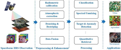
The contiguous spectrum of hyperspectral imagery is its unique advantage over traditional multispectral remote sensing imagery, and has promoted the advancement of new methods of processing hyperspectral images(Zhang and Du 2012). However, due to the high dimensionality (Acito, Diani, and Corsini 2009; Cheriyadat 2003), low spatial resolution (Mianji and Zhang 2011; Chang 2007), spectral mixture problem, and the noise and atmospheric effects, hyperspectral image processing is a challenging task. The processing framework for spaceborne HRS is illustrated in Figure 2, including the data preprocessing (i.e., radiometric calibration and geometric correction), data enhancement (i.e., denoising, destriping, and data fusion), and data processing (i.e., classification, target and anomaly detection, and quantitative retrieval). The recent progress in China in the processing and analysis of hyperspectral imagery is reviewed and analyzed in this section.

Figure 2. The processing framework for spaceborne HRS

3.1. Data preprocessing

3.1.1. Radiometric calibration

Radiometric calibration, as an important component of spaceborne hyperspectral image preprocessing, involves inversing the true spectral radiance or reflectance of the ground surface. According to the state of the sensor, radiometric calibration can be divided into preflight and in-flight calibration (which includes both onboard and vicarious calibration) (Dinguirard and Slater 1999). The main preflight measurements necessary to characterize the sensor are: the absolute radiometric calibration coefficients, the spectral response, and the equalization coefficients (1999). Preflight calibration can be divided into laboratory calibration and field calibration. After the satellite is launched, radiometric calibration of the sensor using calibration equipment on the satellite is called onboard calibration. Vicarious calibration means selecting a certain field from the Earth’s surface as an alternative target during the operation of the satellite, where radiometric calibration of the sensor is achieved through observation of this alternative target.

As the onboard systems have to be monitored to assess their potential degradation, methods based on natural Earth scenes have been developed (Dinguirard and Slater 1999). For example, a vicarious radiometric calibration procedure was established by Zhang et al. (2018) for the SPARK-01 and −02 satellites. This method includes the computation of the dark current and non-uniform correction processes. The dark current computation is achieved by averaging multiple lines of long-strip imagery obtained over wide ocean areas during the nighttime, while the non-uniform correction processes are undertaken using images obtained after modification of the satellite yaw angle to 90°. A field-free relative radiometric calibration method based on the harmonic analysis of yaw data has also been proposed for use with the hyperspectral images acquired by the OHSs, which is called the Harmonic Analysis Radiometric Calibration (HARC) algorithm (Wang, Yang, and Wang 2020).

Certain test sites in China, such as the Dunhuang site located in Gansu province, the Qinghai Lake site situated in Qinghai province, and the Baotou site situated in Inner Mongolia, are commonly used to achieve the absolute calibration of satellite sensors. These sites are extensive, homogenous, and cloud-free, allowing good ground representation, and can be employed as reference reflectance objects.

The Dunhuang site is in Gansu province in the northwest of China. Most areas of the Dunhuang radiometric calibration site have no vegetation, and feature uniform material composition, flat terrain, and high stability and uniformity (Hu et al. 2010). The central area of the site is a synchronous observation area that is used for the satellite calibration. The surface reflection ratio of this area in the VNIR region is about 14–25%, and in the SWIR band it is about 30%. The surface optical property of this area is good, and the reflection ratio changes only slightly. The optical uniformity is further improved with the increase of the observed field of view. The reflectance of the site is basically located in the middle part of the dynamic range of satellite remote sensors, which satisfies the in-orbit radiometric calibration of most satellite remote sensors. As a result, the site is mainly employed for the radiometric calibration of the VNIR bands of remote sensing satellites.

The Qinghai Lake radiometric calibration site is located in the northeast of the Tibetan Plateau. The water surface temperature distribution of Qinghai Lake is uniform, and the temperature change over the lake surface is less than 1°C. The Qinghai Lake radiometric calibration site is at high altitude, where there are few aerosol particles, and the aerosol optical thickness is about 0.1 (Wang et al. 2015b). The Qinghai Lake radiometric calibration site has been widely used in the absolute in-orbit radiometric calibration of remote sensing satellites in the TIR range, and low-reflectance radiometric calibration tests of the VNIR bands can also be carried out.

The Baotou calibration site is located in the central area of Inner Mongolia, and features flat terrain, dry climate, and good atmospheric visibility. It covers an area of 300 km² and has an altitude of 1270 m. The calibration site consists of both desert and permanent artificial calibration targets. There is also an automatic observation system for field spectral characteristics and atmospheric parameters (Pang et al. 2019).

3.1.2. Geometric calibration

Geometric processing is an important component of hyperspectral image preprocessing, where the geometric information of ground objects can be extracted from the hyperspectral images after data preprocessing. According to the acquisition mode of the control information, geometric calibration can be divided into two types: (1) geometric calibration methods based on a ground calibration field; and (2) autonomous geometric calibration methods. Calibration based on a ground calibration field involves using the calibration field image obtained from the satellite in orbit to match with the digital orthophoto image and digital elevation model data of the calibration field to obtain dense control points. The autonomous geometric calibration method uses the sensor in orbit to obtain multiple images of different observation angles, and the connection point information is obtained through image matching, which only needs a few control points, and greatly reduces the dependence on reference data.

Geometric processing methods for Zhuhai-1 hyperspectral satellite data have been proposed, including both geometric correction and basic product production algorithms (Jiang et al. 2019). In the geometric calibration of the GF-5 AHSI camera, the pointing angle of the probe can be used (Mi et al. 2019), the internal and external calibration parameters are solved step by step, and some typical images are selected for experimental verification.

In addition, it is worth mentioning that most of the data preprocessing methods mentioned above can also be used with the data of other spaceborne hyperspectral sensors, in addition to the Chinese spaceborne hyperspectral sensors mentioned in the text.

3.2. Data enhancement

3.2.1. Denoising

With the improvement of the spectral resolution, hyperspectral images are inevitably contaminated by noise, including dead pixels and stripe noise, in the process of acquisition, conversion, transmission, compression, and storage, due to the influence of the imaging equipment (Chang and Du 2004). Hyperspectral image denoising refers to reducing the image noise and improving the image quality through post-processing technology. Compared to natural images, hyperspectral images have the characteristic of high spectral redundancy. However, when used in hyperspectral image denoising, the band-by-band strategy does not utilize the high spectral redundancy of hyperspectral images. In the early days, statistics-based destriping methods were proposed by employing histogram information (Horn and Woodham 1979) and the parameters of the sensors (Gadallah, Csillag, and Smith 2000). Subsequently, filter-based methods employing Fourier filters (Pan and Chang 1992) and wavelet filters (Torres and Infante 2001) have been proposed to remove stripe noise. Rudin et al. 1992 proposed A regularization model to remove Gaussian noise by minimizing the sum of squared gradient. More recently, hyperspectral image denoising has been achieved by employing tensor decomposition (Fan et al. 2018), which maintains the spatial-spectral continuity. Zhang et al. 2019 proposed a method to remove, hybrid noise in hyperspectral images was proposed based on spatial-spectral gradient information. Moreover, learning-based methods using Convolutional Neural Networks (CNNs) (Chang et al. 2018) have also been proposed to remove the noise in hyperspectral images.

Dead pixels often exist in hyperspectral images because of the various malfunctions of the collection system during the scanning and transformation process (Wang, Yang, and Wang 2020). Continuous dead pixels affecting a large number of bands severely hamper the visual image perception and may preclude the use of corrupted hyperspectral images in the subsequent applications. A hyperspectral inpainting method named HyInpaint was proposed to restore the dead pixels for TG-1 hyperspectral VNIR waveband data, in which the original hyperspectral image is represented on a low-dimensional subspace, and its estimation is formalized with respect to the subspace representation coefficients on a given basis (Yao et al. 2017).

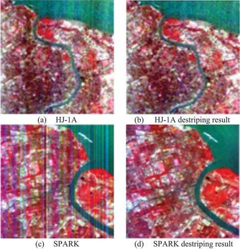
Due to the many degradation factors, including poor atmospheric conditions, defective calibration, and sensor defects, spaceborne hyperspectral images are often polluted by stripe noise (Zhong et al. 2020), which needs to be solved by a destriping technique. In (2020), a Satellite-Ground Integrated Destriping Network (SGIDN) was proposed for the destriping of EO-1 Hyperion imaging spectrometer data, HJ-1A hyperspectral data, and SPARK satellite data, in which a satellite-ground integrated strategy was proposed to obtain a large set of striped-clean pairs, which are required in the learning-based methods. The destriping results obtained by the SGIDN algorithm for the HJ-1A and SPARK HSIs are shown in Figure 3. A unique destriping algorithm for OHS data was also proposed by Li, Zhong, and Wang (2019), in which the adaptive moment matching method and multi-level unidirectional total variation method are used to remove the stripes. A model based on piecewise linear least-squares fitting is then used to restore the vertical details that were lost in the first step.

Figure 3. Visualization of the destriping results for HJ-1A data and SPARK data using the method proposed by Zhong et al. 2020. (a) HJ-1A. (b) HJ-1A destriping result. (c) SPARK. (d) SPARK destriping result

3.2.2. Super-resolution and data fusion

Hyperspectral imaging is often subject to the constraint of the low spatial resolution (Di et al. 2008), which is caused by the mutual restriction between the spectral resolution and spatial resolution in the design of optical remote sensing systems (He et al. 2008). For example, the GF-5 satellite has a spatial resolution of only 30 m, and the HJ-1A satellite has a spatial resolution of only 100 m. Data fusion and super-resolution reconstruction techniques are ways to improve the spatial resolution of hyperspectral images. The data fusion of hyperspectral and multispectral images has become a hot research topic, which is aimed at incorporating the fine spatial context of multispectral images in hyperspectral images. The data fusion methods can be divided into spectral data fusion methods, spatial data fusion methods, spatial-spectral data fusion methods, and multisource data fusion methods. Among the different methods, spectral data fusion is aimed at preserving the most useful spectral information by fusing bands (Jacobson and Gupta 2005); spatial data fusion is concerned with enhancing the spatial resolution of the images by fusing multiple low-resolution images (Zhang, Zhang, and Shen 2012); spatial-spectral data fusion accomplishes super-resolution by the fusion of different parts of the hyperspectral images (Qian and Chen 2012); and multisource data fusion achieves super-resolution by incorporating other available images of a high spatial resolution (Zhang, De Backer, and Scheunders 2009).

Super-resolution reconstruction techniques are another way to improve the spatial resolution of hyperspectral images. Therein, super-resolution reconstruction methods based on deep learning are aimed at learning the mapping from low spatial resolution images to high spatial resolution images. For example, a novel CNN-based framework was proposed by Mei et al. (2017a) for the super-resolution of hyperspectral images by considering both the spatial context and spectral correlation. Furthermore, 3D convolution has been used to exploit both the spatial context of neighboring pixels and the spectral correlation of neighboring bands (Mei et al. 2017b). This allows the spectral distortion to be alleviated when directly applying the traditional CNN-based super-resolution algorithms to hyperspectral images in a band-wise manner.

Ren et al. (2020) provided a comprehensive evaluation of the methods that can be used to fuse GF-5 hyperspectral data with Sentinel-2A, GF-1, and GF-2 multispectral data. The aim of the data fusion was to enhance the GF-5 data with the high spatial resolution multispectral data while preserving the spectral fidelity. This study showed that Lanaras’s method, the Gram-Schmidt Adaptive (GSA) method, and the Modulation Transfer Function (MTF)-Generalized Laplacian Pyramid (GLP) method can all effectively improve the spatial resolution when fusing GF-5 and GF-1 data. The MTF-GLP and GSA methods showed a better effectiveness in incorporating GF-5 and GF-2 data, and GSA and Smoothing Filter based Intensity Modulation (SFIM) were suggested for fusing GF-5 and Sentinel-2A data. A multi-sensor image fusion strategy for GF-5/GF-1 spatial-spectral fusion with a high spatial resolution was proposed by Wei et al. (2015), in which a unified fusion framework for multi-sensor image fusion was derived on the basis of step-by-step fusion theory. In the proposed method, an MTF was applied to separate the spatial (high frequency) and spectral components (low frequency) of the multisource images. The fusion weight was then constructed by comprehensively considering the relationship between the multi-sensor high spatial resolution images and high spectral resolution images and the spectral correlation of the hyperspectral images.

3.3. Classification

Assigning a label to each pixel is a key application in remote sensing technology, and has been widely applied in ground mapping, urban planning, mineral resource exploration, environmental monitoring, military reconnaissance, and other fields (Lv et al. 2015).

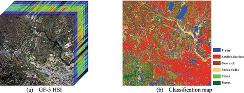
Figure 4 shows the land-cover mapping result obtained using GF-5 hyperspectral images. According to the use of the spatial information, the classification methods can be divided into two approaches: (1) spectral classification methods; and (2) spectral-spatial classification methods (Ghamisi et al. 2017b).

Figure 4. The hyperspectral image classification task. (a) GF-5 HIS. (b) classification map

For the spectral classifiers, each pixel of a hyperspectral image is considered to be a combination of a series of spectral measurements that do not contain spatial information. Ghamisi et al. 2017a compared the most widely used spectral classifiers in depth, including Support Vector Machine (SVM) (Melgani and Bruzzone 2004), Random Forest (RF) (Gislason, Benediktsson, and Sveinsson 2006), the back-propagation neural network (Benediktsson, Swain, and Ersoy 1990), extreme learning machine (Pal 2009), rotation forest (Xia et al. 2014), canonical correlation forest (Xia, Yokoya, and Iwasaki 2016), and a one-Dimensional (1-D) deep CNN (Chen et al. 2014b). In recent hyperspectral image studies, deep learning has made a great contribution. Compared to the shallow models, high-level, hierarchical, and abstract features are extracted from the deep learning models. The autoencoder model is a typical kind of deep learning based hyperspectral image classification approach. Examples of autoencoder models are the stacked autoencoder (2014b) and an autoencoder with sparse constraint (Tao et al. 2015). Deep belief networks have also been used for classification by learning spectral-based features (Chen, Zhao, and Jia 2015).

In a spectral-spatial classifier, the hyperspectral image is classified by considering the spatial dependencies of adjacent pixels. Spatial information can be used in hyperspectral image classification in many ways. Ma et al. 2014 proposed a mixed classification method which incorporates spatial information by the fusion of object-based segmentation with SVM. This method uses two mixed classification strategies – the multi-resolution segmentation algorithm and multi-scale watershed segmentation – which were applied to TG-01 hyperspectral urban data. Spatial-spectral joint contextual sparse coding has also been proposed for hyperspectral image classification (Lv et al. 2015), and includes three main parts: (1) dictionary construction; (2) sparse coefficient solving; and (3) SVM classification. In this method, a dictionary is first obtained by training the samples selected from the ground-truth data, and then the sparse coefficients of each pixel are calculated based on the learned dictionary. The sparse coefficients are then input into the SVM classifier and the final classification result is obtained. Jiao et al. 2019 applied a hierarchical classification framework in the classification of coastal wetlands, where a decision tree was used to extract the land-cover types (buildings, crops, plants, and wetlands) and SVM was used to classify subtypes with the spectral and spatial information. As one of the most active research fields in the computer science field, deep learning has shown excellent performances in many tasks (Ma et al. 2014). For example, a novel cascade forest model was proposed by Qi et al. (2019) to overcome the limitations of the traditional deep neural networks, such as the requirement for a lot of training samples and the optimization of a large number of hyperparameters. The improved cascade forest model is an accumulation of layers, with each layer consisting of two decision tree forests and a logistic regression classifier. Compared with the traditional model, the number of forests in the improved method is reduced from four to two, with the same accuracy and efficiency.

In spatial-spectral feature fusion, deep learning based approaches have shown better performances than the traditional machine learning algorithms (Lv et al. 2015). According to the CNN model, the deep learning based methods can be divided into patch-based and fully convolutional neural network based methods. Qi et al. 2019 proposed a joint classification framework of a 3D CNN and a Convolutional Longshort Term Memory (CLSTM) network called SSCC, for hyperspectral image patch-based classification, in which the 3D CNN was used to learn the spectral-spatial features and then the sequence features were extracted by CLSTM. In order to avoid the redundant calculation in the patch-wish classification methods and use the global spatial information, fully convolutional neural networks have been introduced into hyperspectral image classification. Since the training samples for hyperspectral images are often very sparse, and the traditional training strategy in the fully convolutional neural networks is no longer suitable for hyperspectral image classification, Xu et al. 2020 proposed a mask matrix to assist the back-propagation in the training stage. A global stochastic stratified sampler was proposed by Zheng et al. (2020) in the Fast Patch-free Global leArning framework (FPGA). The Conditional Random Field (CRF) model can also be used to further balance the local and global information in fully convolutional neural networks (Xu, Du, and Zhang 2020; Alam et al. 2017).

3.4. Target detection and anomaly detection

The hyperspectral target detection methods can be generally classified into two categories – anomaly detection based methods and signature-based target detection methods (Nasrabadi 2014) – according to whether or not prior knowledge of the materials of interest is available.

3.4.1. Signature-based target detection

For the signature-based target detection methods, the signatures of the targets are known in advance. The traditional signature-based target detection methods are derived from binary hypothesis testing. That is, for each pixel, two hypotheses exist: the H₀ (target absent) and H₁ (target present) hypotheses (Manolakis, Marden, and Shaw 2003). In addition, specific statistical distributions can be utilized to approximate the hyperspectral data distribution, such as a Gaussian distribution (Trebesch and Kolb 2009) or chi-square distribution (Du and Zhang 2011). The Likelihood Ratio (LR) (Lee and Carder 2007) or Generalized Likelihood Ratio (GLR) test (Kraut and Scharf 1999) is then employed to construct a constant false alarm rate detector. Typical methods include the various subspace detection algorithms, such as the Orthogonal Subspace Projection (OSP) approach (Harsanyi and Chang 1994), the Matched Subspace Detector (MSD) (Scharf and Friedlander 1993), and the Adaptive Coherence/Cosine Estimator (ACE) (Kraut and Scharf 1999; Manolakis 2005). The OSP approach involves constructing the subspace orthogonal to the background subspace to realize suppression of the background. The MSD constructs the target and background subspace and then constructs the GLR detector. The principle of ACE is similar to that of MSD, but the method used to construct the subspace is different.

More recently, sparse representation has been successfully applied in target detection. The sparsity-based detectors are based on the principle that the background lies in a low-dimensional background subspace, while the target lies in a low-dimensional target subspace. Sparse representation was first applied in hyperspectral target detection by Chen, Nasrabadi, and Tran (2011a). Based on the basic principles and methods, many improved algorithms have since been proposed (Chen, Nasrabadi, and Tran 2011b, 2011c; Li et al. 2014). In these sparsity-based algorithms, the target and background dictionaries are constructed using the training samples to represent the target and background, respectively. Owing to the completeness of the constructed dictionaries, many atoms are employed to describe one kind of material, thus solving the spectral variability problem (Sakla et al. 2011). In addition, to further exploit the spatial information in hyperspectral images while solving the spectral variability problem, sparse representation models have been combined with the spatial-contextual models (Gu et al. 2015; Zhao et al. 2013; Wu et al. 2019; Zhang et al. 2017), in which the spatial neighborhood information in the adaptive local windows or adjacent neighborhoods is exploited.

3.4.2. Anomaly detection

Anomaly detection is aimed at detecting the observations which have significant differences with the surrounding background in spectral characteristics (Stein et al. 2002). For the anomaly detection methods, contrary to the signature-based target detection methods, no a priori signatures are available about the anomalies (Manolakis 2005). In this case, the background estimation and suppression becomes a crucial issue in the hyperspectral anomaly detection task (Matteoli et al. 2013). To address this issue, the statistical methods utilize prior statistical distributions for the background estimation. Examples of such methods are the well-known Reed-Xiaoli (RX) detector (Reed and Yu 1990) and its improved methods, which are all based on the Mahalanobis distance, including the regularized RX detector (Nasrabadi 2008), the segmented RX detector (Matteoli, Diani, and Corsini 2010), the weighted RX detector, and the linear filter based RX detector (Guo et al. 2014). However, as the statistical distribution assumptions are usually inconsistent with real data, representation-based methods have also been proposed. For example, Pang et al. (2015) proposed a collaborative representation based detector based on the observation that a background pixel can be approximately represented as an linear combination of its surrounding pixels, while the anomalies cannot.

In hyperspectral images, it is generally assumed that the background exhibits a low-rank property while the anomalies are sparse. Therefore, the low-rank prior (Donoho 2006; Wright et al. 2009; Candes et al. 2011) has been introduced into hyperspectral anomaly detection, forming the low-rank based methods. In the low-rank based methods, the hyperspectral anomaly detection problem is modeled as a low-rank and sparse matrix decomposition problem, thus separating the anomalies from the background. The low-rank based methods can be generally classified into two categories: (1) Robust Principal Component Analysis (RPCA)-based methods (Sun et al. 2014; Zhang et al. 2015); and (2) Low-Rank Representation (LRR)-based methods (Yang et al. 2016; Ying et al. 2018; Huyan et al. 2019). The RPCA-based methods directly put the low-rank and sparse constraints on the original hyperspectral data matrix. An example of such a method is the Low-Rank and Sparse Matrix Decomposition (LRaSMD)-based Mahalanobis Distance method for hyperspectral Anomaly Detection (LSMAD) (Zhang et al. 2015). Unlike the RPCA-based methods, the LRR-based methods put the low-rank and sparse constraints on the sparse coding coefficient matrices, which come from the sparse coding of the hyperspectral data based on the spectral dictionaries. Examples of the LRR-based methods are the anomaly detection method based on Low-Rank and Sparse Representation (LRASR) (Yang et al. 2016) and the Abundance- and Dictionary-based Low-Rank decomposition (ADLR) (Ying et al. 2018) method.

More recently, autoencoders have been applied in hyperspectral anomaly detection (Zhao, Li, and Zhu 2017; Zhao and Zhang 2018; Chang, Du, and Zhang 2019; Lu, Zhang, and Huang 2019; Xie et al. 2019) as autoencoders can learn hierarchical, abstract, and high-level representations of hyperspectral data. The autoencoder based methods utilize an autoencoder to automatically extract the latent features of the imagery, and then detectors are designed to realize the final anomaly detection. For example, a Spectral Constrained Adversarial Autoencoder (SC_AAE) was proposed by Xie et al. (2019), in which a spectral constraint strategy is incorporated into an adversarial autoencoder to learn the latent representation of the preprocessed hyperspectral data, and then a bi-layer architecture is used to realize anomaly detection.

3.5. Spectral unmixing

Due to the effect of the low spatial resolution, the multiple scattering of photons, and microscopic mixing, hyperspectral images suffer from serious mixture effects (Bioucas-Dias et al. 2012). As a result, there are often many mixed pixels containing more than one material in hyperspectral images. Spectral unmixing is a procedure that decomposes the mixed pixel into endmembers (the spectral signatures of the materials) and abundances (the relative contributions of the materials). Spectral unmixing is a useful way to analyze hyperspectral data, in applications such as planetary science chemometrics, materials science, and other areas of micro-spectroscopy in medicine (Dobigeon et al. 2013). More precisely, unmixing is a generalized inverse problem that uses the observed signal to estimate parameters to describe an object (Tarantola and Valette 1982). When the incoming light interacting with all the materials within the instantaneous field of view, various physical interactions may occur, so that the observed pixel spectrum is affected (Heylen, Parente, and Gader 2014).

Generally speaking, there are to main two categories of mixing models: (1) the Linear Mixing Model (LMM); and (2) the Nonlinear Mixing Model (NMM) (Keshava and Mustard 2002). The LMM is more likely to occur in macro-spectral mixture scenes where the observed photons mainly interact with a single material before reaching the sensor. In the NMM, which is often present in intimate scenes, the mixing relationship of the different components is nonlinear as the light photons scatter with more than one component. In most cases, the NMM is superior to the LMM, in that it can better describe the actual interactions occurring at the Earth’s surface.

Spectral unmixing based on the LMM can be generally divided into two steps: (1) endmember extraction; and (2) abundance inversion. The endmember extraction is aimed at extracting a relatively high-content feature spectral vector from the HRS imagery. Geometrical-based approaches obtain the vertex by finding the minimum volume or maximum volume of the simplex, to obtain the desired endmember. Examples of such methods are the pixel purity index (PPI) (Boardman, Kruse, and Green 1995), Vertex Component Analysis (VCA) (Nascimento and Dias 2005), N-FINDR (Michael 1999), and the Minimum Volume Enclosing Simplex (MVES) (Chan et al. 2009). The spectral unmixing problem can also be turned into a Blind Source Separation (BSS) problem. For the Iindependent Component Analysis (ICA) method (Bayliss, Gualtieri, and Cromp 1998), it assumes that the multidimensional observation signal is made up of several statistically independent components. However, the sum-to-one constraint of the abundance means that the components cannot be independent, so Nonnegative Matrix Factorization (NMF) can be used to deal with the blind hyperspectral unmixing problem. Some state-of-the-art blind unmixing approaches, such as L_1/2 sparsity-constrained NMF (L_1/2 NMF) (Qian et al. 2011) Minimum-Volume-Constrained NMF (MVCNMF) (Miao and Qi 2007), and Spatial Group Sparsity-Regularized NMF (SGSNMF)(Wang et al. 2017b), take advantage of NMF. Sparse unmixing assumes that the HRS imagery can be taken into account as a linear sparse regression problem. The Sparse Unmixing via variable Splitting and Augmented Lagrangian (SUnSAL) algorithm (Iordache, Bioucas-Dias, and Plaza 2011) was proposed to solve the linear sparse spectral unmixing problem. To make full use of the spatial information in the imagery, a number of spatial based sparse unmixing algorithms have also been developed, such as Non-Local Sparse Unmixing (NLSU) (Zhong, Feng, and Zhang 2013) and Sparse Unmixing via variable Splitting and Augmented Lagrangian with total variation (SUnSAL-TV) (Iordache, Bioucas-Dias, and Plaza 2012) .

Radiative Transfer Theory (RTT) (Chandrasekhar 1960) can describe the energy transformation when the observed photons interact with the components in the scene. However, the complete physics-based nonlinear unmixing approach requires prior information about the scene, which may be difficult or even impossible to obtain. Bilinear models have also been proposed (Fan et al. 2009; Halimi et al. 2011; Altmann et al. 2012) to handle the second-order scattering effects. These models introduce additional interaction terms based on the standard linear model. The main difference is that they impose different mixing parameters on the additivity constraints. It can be found that, for the observed spectral signal, the multiple interactions of photons start to play a significant role, and third-order or higher reflections can no longer be simply ignored. Therefore, methods which consider high-order interactions have also been proposed (Heylen and Scheunders 2016; Wei et al. 2017; Yang and Wang 2018).

With the development of deep learning, the data driven advantages have been considered in many methods. An unsupervised Enhanced Nonlinear Autoencoder (ENAE) method (Zhu et al. 2019) was proposed for the nonlinear unmixing of GF-5 data. This method includes two phases, where the first phase is the initialization of the network structure, which determines the number of nodes of the encoder and the initial values of the endmembers and abundances, and the second phase is the nonlinear unmixing, which mainly involves the minimization of the loss function.

Remote sensing provides us with the possibility to monitor ecosystems and the environment at a large scale (Hadeel et al. 2011). Liao et al. 2012 utilized unmixing to improve the retrieval of the fractional vegetation cover information of Shihezi area in Xinjiang by using hyperspectral data acquired by the HJ-1A satellite. The authors selected the endmember spectra by combining the Endmember Average Root-mean-square error (EAR) and the PPI. Mangrove is typical vegetation found at the junction of land and sea, and is very important for the ecological protection of the waterfront and surrounding areas. Wang et al. (2017a) proposed a method based on hyperspectral unmixing to recognize mangrove by experiments with data from the region of Shenzhen Bay, which were obtained by the TG-1 platform. Marzi et al. (2019) proposed a scheme to provide accurate estimations of the mineral abundance distributions on the lunar surface. Furthermore, they provided detailed information on the lunar surface geophysical composition.

3.6. Quantitative retrieval

Hyperspectral images have nearly continuous spectral information, providing the possibility of the retrieval of surface material properties. Chinese hyperspectral data have been applied to atmospheric parameter retrieval (Xiangchao et al. 2020; Chen et al. 2018), vegetation attribute retrieval (Yang et al. 2017), and surface temperature retrieval (Chen et al. 2017; Ye et al. 2017; Ren et al. 2018; Chen et al. 2014a).

3.6.1. Atmospheric parameter retrieval

Optimal estimation theory (Xiangchao et al. 2020) is one of the most popular theories for atmospheric parameter retrieval. The observation vector y denoting all the measurements can be used to retrieve the state vector $x$through the following formula:

(1) $y=F(x)+\xi$(1)

where F is a forward function modeling the physical process of the observed Top-Of-Atmosphere (TOA) quantity detected by the satellite, with $\xi$ being the errors from the instrument.

The inversion problem can be summarized as a Gaussian probability density function based on a Bayesian approach, and the information content contained in the observation vector can be indicated by the averaging kernel matrix A:

(2) $A=\frac{\mathrm{\partial }\hat{x}}{\mathrm{\partial }x}=(K^T{S}_{\xi }^{-1}K+S_a^{-1}{)}^{-1}{K}^T{S}_{\xi }^{-1}K$(2)

In (2) the averaging kernel matrix $A$ is the calculation result of the weighting function matrix $K$, the prior error $S_a$, and the measurement error covariance matrix $S_{\xi }$showing the sensitivity of the retrieval to the true state. The weighting function is the partial derivative of the forward model to the state vector $K_{ij}=\mathrm{\partial }{F}_i/\mathrm{\partial }{x}_{\mathrm{\partial }j}$, where $i$ and $j$represent the $i$th measurement $F_i$ and the $j$th element in $x$. The closer the diagonal elements of $A$ are to 1.0, the more information content can be contained by the corresponding parameters. The trace of $A$ is called the Degrees of Freedom for the Signal (DFS), which represents the number of independent pieces of information provided by the observation vector. The prior uncertainty of the retrieved parameter is reduced with the increase of the measurements, and this error reduction represents the amount of information provided by the observations. The a posteriori error covariance matrix $\hat{S}$ can be described as:

(3) ${\hat{S}}^{-1}=K^T{S}_{\xi }^{-1}K+S_a^{-1}$(3)

The square root of its diagonal elements is the errors of the retrieved parameters. Thus, information on aerosols, gases, and surface properties can be obtained from the DFS and error reduction between the a priori error and the a posteriori error (Chen et al. 2018). The Aerosol Optical Depth (AOD) is another parameter that can be retrieved from hyperspectral data, and is commonly used to achieve extensive and rapid monitoring of particulate matter distributions (2018). The dark target inversion algorithm for HJ-1 CCD data primarily involves the expression for the apparent reflectance at the TOA. Under the horizontally homogeneous and vertically non-homogeneous assumption about the atmosphere, the apparent reflectance at the TOA can be expressed by:

(4) ${\rho }_{TOA}={\rho }_a({\mu }_S,{\mu }_V,\phi )+\frac{T({\mu }_S)\cdot T({\mu }_V)\cdot \rho ({\mu }_S,{\mu }_V,\phi )}{1-S\cdot \rho ({\mu }_S,{\mu }_V,\phi )}$(4)

where ${\rho }_{TOA}$ is the apparent reflectance at the TOA; ${\rho }_a({\mu }_S,{\mu }_V,\phi )$ is the atmospheric reflectivity; $\rho ({\mu }_S,{\mu }_V,\phi )$ is the albedo; ${\mu }_S=cos{\theta }_S$; ${\mu }_V=cos{\theta }_V$; ${\theta }_S$ and ${\theta }_V$ are the solar zenith angle and zenith observation angle, respectively; $\phi$ is the relative azimuth angle; $T$ is the total transmittance; and $S$is the atmospheric albedo.

3.6.2. Plant property retrieval

A robust, accurate, and operational scheme based on Synthetic Aperture Radar (SAR) and HRS data (HJ-1A/B) was proposed for rice phenology estimation by Yang et al. (2017), in which 149 SAR features and Vegetation Indices (VIs) were extracted by using a time series of optical and SAR data. The multiclass relevance vector machine was then used to identify the different stages. The common vegetation indices are listed in Table 12.

Table 12. Common vegetation indices

Method	Formulation
NDVI (Huete et al. 2002)	(NIR-Red)/(NIR + Red)
RVI (Elvidge and Chen 1995)	NIR/Red
EVI (Huete et al. 2002)	2.5(NIR-Red)/(NIR+6Red-7.5Blue+1)
GNDVI (Hunt et al. 2010)	(R750-R550)/(R750+R550)
NPCI (Penuelas et al. 1994)	(R680-R430)/(R680+R430)
NDRE (Tian et al. 2011)	(NIR-Rededge)/(NIR+Rededge)
MTCI (Dash and Curran 2004)	(NIR-Rededge)/(Rededge-Red)
SAVI (Qi et al. 1994)	(NIR-Red) (1 + L)/(NIR + Red + L)

3.6.3. Surface temperature retrieval

Land Surface Temperature (LST) is important for studying the exchange of energy between the land surface and the atmosphere (Chen et al. 2017). The quadratic split-window approaches have been widely used in LST estimation. However, when estimating the LST with low land surface emissivity, the performance of the quadratic split-window method is poor. In order to solve this problem, Chen et al. (2017) assumed that the land surface emissivity is a fixed constant, and calculated the LST with the quadratic split-window method by keeping the other coefficients the same as those obtained under the black body condition. In order to avoid the effect of the atmosphere on LST estimation, a nonlinear four-channel split-window algorithm was proposed by Ye et al. (2017) to retrieve LST from GF-5 data. In addition, under different land surface conditions, the coefficients of the split-window algorithm were estimated based on several subranges of the atmospheric Column Water Vapor (CWV). The LST and sea ST (SST) have also been estimated using a Different Thermal Channel Combination Split-Window (DTCC-SW) method, which was proposed by Tang (2018) for use with GF-5 satellite TIR data, in which some different thermal channel combinations were proposed to estimate the surface emissivity under different conditions. The Temperature and Emissivity Separation (TES) algorithm is another widely used LST estimation algorithm. However, the TES algorithm has a high requirement for atmospheric correction of the TIR data, and the TES algorithm performs poorly when the emissivity of the surface is low. A hybrid algorithm was proposed by Ren et al. (2018) to combine the quadratic split-window and TES methods, and improve the performance of LST estimation, in which the initial LST and emissivity are obtained by the TES algorithm. The new LST is then obtained through the split-window algorithm with this emissivity, and the new LST is then applied to the TES algorithm again to obtain a more refined LST.

Total Suspended Matter (TSM) can also be retrieved from hyperspectral imagery. The TSM concentration has been retrieved by a three-band semi-analytical model from a coastal water area with HJ-1A data (Chen et al. 2014a), where the TSM can be described as follows:

(5) $C_{TSM}\propto \frac{s(660)}{s(560)-{\epsilon }_{aa}{\epsilon }_{bb}s(485)}$(5)

where $s(\lambda )$ is the ratio of the total backscattering coefficient to the total absorption coefficient at a certain wavelength, and ${\epsilon }_{aa}=1.6498$ and ${\epsilon }_{bb}=0.4237$.

4. Applications of chinese hyperspectral satellites

In view of the high accuracy and strong ability to identify different features, HRS can be used to accurately distinguish different ground types and achieve quantitative inversion, thus supporting the applications of natural resource investigation, urban construction management, agricultural production, and ecological environment monitoring. The rapid development of Chinese hyperspectral satellite technology is aimed at meeting the major national needs such as pollution reduction, environmental quality supervision, atmospheric composition and climate change monitoring, and land and resource surveying, while promoting the application of HRS in agriculture, forestry, disaster reduction, urban construction, water conservancy, marine studies, surveying and mapping, statistics, and other departments. The following section introduces the typical applications of Chinese HRS satellites in these fields.

4.1. Agricultural applications

At the time of writing, precision agriculture has become the main goal and direction of China’s National Agricultural Modernization Plan (2016–2020). HRS technology, as a simple, fast, low-cost, and nondestructive spectral analysis technique, has attracted much attention in precision agriculture applications. HRS has been used to monitor crop growth, crop physiological and biochemical characteristics, and to estimate crop area and yield, providing a guarantee for the planting and management of crops (Zhang and Li 2019; Shi et al. 2017; Chong et al. 2017).

The growth and health of crops over time can be established by analyzing the physiological parameters of the crops in different periods, which can be predicted by the spectral reflectance of the crops. The Leaf Area Index (LAI) is not only an important core parameter of crop structure, but is also one of the key parameters in climate and ecological research. Li et al. (2016b) predicted the continuous changes of winter wheat LAI by extracting a variety of features from HJ-1 A/B CCD images of four winter wheat growing seasons. Another important crop parameter – nitrogen content – which plays a key role in plant photosynthesis, can reflect the nutritional status of crops. For example, Zhou et al. (2016) used PHI airborne hyperspectral data to conclude that “Normalized Difference Vegetation Index (NDVI)-like” indices are the best indices for estimating winter wheat Canopy Nitrogen Content (CNC). Liang et al. (2018) also developed new hyperspectral indices – the First Derivative Normalized Difference Nitrogen Index (FD-NDNI) and the First Derivative Ratio Nitrogen vegetation Index (FD-SRNI) – and estimated the Leaf Nitrogen Content (LNC) of wheat from OMIS imagery.

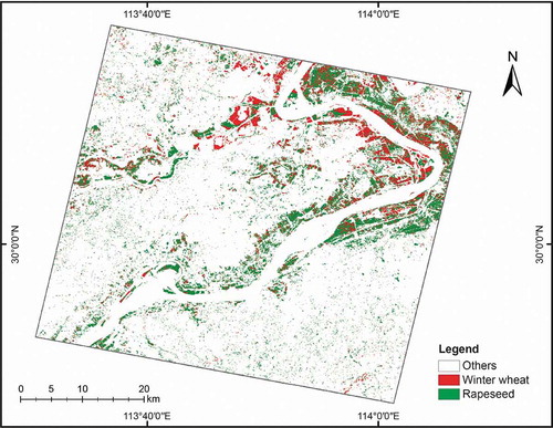
The crop classification and mapping techniques based on hyperspectral images are well established and can help us to acquire the timely crop planting information of a large area. The authors utilized OHS hyperspectral data in the peak period of crop growth to realize the classification of winter wheat and rapeseed. As shown in Figure 5, the crop classification result for the Zhuhai-1 OHS data indicates the feasibility of using Zhuhai-1 OHS data in fine crop mapping in large areas. Shi et al. (2017) utilized the spectral characteristic variables extracted from HJ-1A data to classify different crops in the Huang watershed in Qinghai province by using the SVM method after band selection. Zhang and Li (2019) used OHS hyperspectral images to realize the fine classification and acreage estimation of winter wheat using maximum likelihood and SVM methods. Yang et al. (2008) established a spectral response and detection model for crop disaster based on PHI hyperspectral images, and combined this with the Spectral Angle Mapper (SAM) method to accurately classify and map both wheat affected by stripe rust and healthy wheat. In addition, Pan et al. (2015) obtained a phenological map of farmland in the Guanzhong Plain of China by extracting the NDVI from an HJ-1A/B CCD image time series. Such large-area crop mapping can provide effective support for agricultural management.

Figure 5. Crop classification in the city of Xiantao in China using OHS hyperspectral imagery

The estimation of crop yield is the main way to realize the output value of agriculture. This can be predicted indirectly by inverting the characteristic parameters of crops. For example, Wang et al. (2015a) used multi-temporal HJ-1 A/B CCD images to extract a two-band enhanced vegetation index (EVI2) to predict single-cropped rice yield; and Song et al. (2004) used PHI hyperspectral data to extract the NDVI and Photochemical Reflectance Index (PRI) to establish a winter wheat yield prediction model. The use of airborne imaging spectrometers can be used to monitor crops more accurately, because of the high spatial resolution.

4.2. Forestry applications

Hyperspectral satellite data can also be used in forestry, including forest investigation, forest biochemical composition studies, forest health status research, forest disaster analysis, and alien species monitoring. Chinese hyperspectral satellite data have made great contributions to the development of forestry in China through the applications of forest mapping (Wan et al. 2020), forest resource surveying (2020), and biochemical and physical factor estimation (Chen et al. 2015).

Forest investigation is mainly realized by forest type classification. HRS imagery can improve the classification accuracy of forest species, and a more accurate forest species distribution map can be obtained using hyperspectral data classification. For example, by the use of GF-5 hyperspectral data, Wan et al. (2020) obtained high-precision classification maps of four types of mangroves in the Mai Po Nature Reserve (MPNR) of Hong Kong, and concluded that GF-5 data have the potential to improve species-level mangrove monitoring. Xi et al. (2019) realized the fine distinction of seven different tree species in the Changbai Mountains of Northeast Asia by using OHS-1 data, and concluded that the combination of a deep learning framework and hyperspectral images can effectively improve the accuracy of tree species classification, thus helping to reduce the uncertainties in the estimation of ecosystem parameters and forest resources. Zhao et al. (2018) used PHI-3 hyperspectral data to calculate seven vegetation indices representing key biochemical characteristics. These were then combined with other features for adaptive Fuzzy C-Means (FCM) clustering, to directly predict the diversity of forest species without distinguishing each individual tree species.

The LAI estimation of tree species is also of great significance in forest surveying, resource management, ecological research, and post-disaster assessment. For example, Chen et al. (2015) used HJ-1A/B CCD images to predict the spatio-temporal LAI variation of rubber forest in Hainan, China, by a nonlinear autoregressive network with exogenous inputs (NARX).

4.3. Geological exploration

Hyperspectral satellites can be used to survey the typical minerals and major rock types as different minerals have different spectral responses. The development of Chinese hyperspectral satellites has made a great contribution to geological research in China, especially in mineral identification and mapping, lithologic mapping, mineral resources exploration, mining environment monitoring, and the ecological restoration and evaluation of mining areas (Lei et al. 2018; Liu et al. 2018; Yang et al. 2018).

Mineral identification and mapping are the basis of hyperspectral geological applications, and can provide material information on the composition and distribution of ground objects for geological applications, both macroscopically and regionally. For example, Lei et al. (2018), Liu et al. (2018) realized a large-area routine geological survey with a resolution of 20 m in the main gold-copper-nickel-chromium resource belt of China using TG-1 Hyperspectral Imager SWIR data. This study showed that it is possible to quickly carry out a spaceborne survey of altered minerals (muscovite, kaolinite, chlorite, epidote, calcite, dolomite, etc.) and provide continuous high-accuracy mineral mapping products for all types of topography. These results also suggest that TG-1 data seem to be very suitable for the detection of surface mineralogy, to support regional mapping and exploration. In addition, Yang et al. (2018) realized the fine classification of silicate, carbonate, and sulfate minerals using GF-5 TIR hyperspectral data. However, the application of HRS data in the quantitative inversion of mineral content needs to be strengthened.

4.4. Environmental monitoring

Rapid economic development and human activities are accompanied by a series of environmental pollution problems, and the role of HRS in environmental monitoring is becoming more and more important. Hyperspectral satellites can be used to monitor the environment of water, soil, and air, to meet the needs of environmental protection, monitoring, supervision, emergency response, evaluation, planning, and other fields.

4.4.1. Air pollution monitoring

Climate change has become a global issue of general concern to the international community, which demands prevention and control of air pollution and improvement of atmospheric environmental quality. Hyperspectral satellites can carry out high-accuracy and quantitative remote sensing monitoring of atmospheric environmental elements such as nitrogen dioxide, sulfur dioxide, atmospheric aerosols, and greenhouse gases, allowing us to determine the spatial distribution and concentration of atmospheric pollutants at a large spatial scale. The Environmental Trace Gases Monitoring Instrument (EMI) carried on the GF-5 satellite measures the backscattered terrestrial solar radiation in the ultraviolet and visible spectral range. Cheng et al. (2019) used the EMI to realize the global inversion of nitrogen dioxide (NO₂), which is an important polluting gas, supporting air quality monitoring. The Atmospheric Infrared Ultraspectral Sounder (AIUS) is an infrared occultation spectrometer equipped on the GF-5 satellite that can measure and study the chemical processes of ozone (O₃) and other trace gases in the Antarctic upper troposphere and stratosphere. Li et al. (2019) used the trace gas retrieval algorithm developed for the AIUS and generated the first results for O₃, water, and Hydrogen Chloride (HCl) retrieval from the AIUS, which were used to study the spatio-temporal variation of ozone over Antarctica.

4.4.2. Water environment monitoring

Water is the source of life, and the prevention and control of water pollution is closely related to human health (DATTA et al. 2012). HRS water quality monitoring is realized by the inversion of different water quality parameters which can reflect water pollution, such as chlorophyll, suspended solids, transparency, and turbidity, because the optical properties of these water quality parameters can be reflected by hyperspectral sensors. As early as 2000, Shu et al. (2000) used OMIS-II airborne hyperspectral data to retrieve chlorophyll concentration.

The HJ-1A/B hyperspectral satellites are a common data source for water environment monitoring. For example, Lu et al. (2011) combined the NDVI and Normalized Difference Water Index (NDWI) to realize water body extraction and mapping; Zhou et al. (2014) estimated the concentration of chlorophyll a (chl-a) based on the semi-analytical three-band algorithm; and Cao et al. (2018) used a model coupled with a modified discrete binary particle swarm optimization algorithm utilizing the catastrophe strategy and partial least squares (MDBPSO-PLS) to retrieve water quality indices, including chl-a, TSM, and turbidity.

The AHSI instrument carried on the GF-5 satellite also has great potential in water color remote sensing research because of its high spatial resolution and large number of spectral bands. These characteristics make ASHI data conducive to obtaining subtle changes in inland water quality parameters. For example, Liu et al. (2019a) realized the classification of many kinds of water bodies, including river, sea, salt marsh, and ditch, by using AHSI data; and Deng et al. (2018) established cross-order multi-band inversion models of chl-a concentration based on GF-5 data, realizing high-accuracy chl-a inversion in turbid water with complex optical properties.

4.4.3. Soil property monitoring

Soil properties, such as organic matter, iron oxide content, and nutrients (which are key variables affecting vegetation growth) and the pollutants represented by heavy metals can be reflected by their specific spectral responses. Therefore, HRS can be used to retrieve soil parameters to monitor soil health and pollution, so as to protect agricultural production and the ecological environment.

Yu et al. (2018) used the stepwise regression model of enhanced spectral variables to produce spatial distribution maps of soil properties (organic carbon, total nitrogen, total potassium, and total phosphorus) using HJ-1A images. Li et al. (2015) predicted soil salt content by generating the NDVI, the Normal Soil Salt Content Response Index (NSSRI), and the Soil Adjusted Vegetation Index (SAVI) based on HJ-1A images. Liu et al. (2016) used multi-temporal HJ-1B data to retrieve the heavy metal composition of soil used for growing rice. They also designed a stress index as an indicator for the degree of heavy metal stress on the rice in the different growth stages, and determined the heavy metal stress levels of rice using a Time-Spectrum Feature Space (TSFS) model. Liu et al. (2019c) derived a model considering the relationship of the spectral ratio of Dry Soil Spectral Reflectance (DSSR) to Moisture Soil Spectral Reflectance (MSSR) with soil water content using HJ-1A data, and realized estimation of the soil heavy metal content (ardennite (As), cadmium (Cd), mercury (Hg)).

4.5. Urban research

The rapid and high-intensity urbanization process has significantly changed the urban, regional, and even global ecological environment. One of the remarkable characteristics of the urban climate is the urban heat island effect. HRS can be used to monitor the urban climate and environment mainly by retrieving LST.

Xu, Wooster, and Grimmond (2008) used OMIS data to produce maps of sensible heat fluxes in urban areas at various spatial scales based on the Local-Scale Urban Meteorological Parameterization Scheme (LUMPS) and Aerodynamic dRag Method (ARM). OMIS data can also be used to obtain urban land-cover information and retrieve maps of key surface parameters (albedo, surface temperature, vegetation fraction, emissivity). Meng and Cheng (2020) used high spatial resolution TIR data from the GF-5 satellite to estimate LST through the National Oceanic and Atmospheric Administration Joint Polar Satellite System enterprise algorithm and the quadratic split-window algorithm. In addition to monitoring the urban heat island effect, there are other typical applications related to the urban environment. For example, Li et al. (2016a) used TG-1 data classification methods combined with a pixel-based classifier and object-based segmentation method to obtain accurate urban coverage maps, which can be used to support urban climate change modeling.

5. Conclusions

In recent decades, spaceborne HRS has shown rapid development in China, along with the growth of the satellite and hyperspectral imaging technologies, and has shown great potential in various remote sensing applications. Meanwhile, hyperspectral image processing has been a hot research topic in China and has attracted the attention of scholars in various fields, including remote sensing, signal processing, and the geosciences. In this paper, we have provided a comprehensive review of spaceborne HRS in China, from the aspects of the spaceborne HRS platforms and the corresponding hyperspectral image processing and applications. To end the discussion, in the following, we summarize the main development trends in spaceborne HRS in China:

1. The wide swath width and high spatial resolution. Since the detector array size is limited, there is a tradeoff between the swath width, the spectral resolution, and the spatial resolution of a hyperspectral imager, and it is difficult to improve them simultaneously. However, it is of great value to improve the spatial resolution of spaceborne HRS while maintaining its fine spectral resolution and wide swath width.

2. Hyperspatial observations with a full spectral range. The VNIR (0.4–1.0 μm) and SWIR (1.0–2.5 μm) regions are the commonly used spectral ranges for spaceborne HRS, but from the aspect of applications, it is of value to extend the spectral range to the mid-wave infrared (MWIR, 3–5 μm) and the long-wave infrared (LWIR, 7–12 μm) regions.

3. Hyperspectral satellite networks. The concept of satellite networks has provided a new direction for microsatellites, as well as spaceborne HRS. The Zhuhai-1 satellite network is a typical example, where the joint observation of its 10 OHSs makes it possible to cover the Earth every 2 days and 182 times a year, which greatly improves the temporal resolution of the HRS observations.

In the future, China will continue to develop and launch spaceborne hyperspectral satellites. The FY-3E satellite is expected to be launched in 2021, carrying the MERSI-2 sensor. The fourth batch of OHSs is also in development. In addition, the China Great Wall Industry Corporation has signed a satellite launch contract with Satellogic to launch 90 satellites, and 10 satellites have been in orbit since January 2020. Over the next two years, more than 80 satellites will be launched to form a constellation of Earth observation satellites, each of which will carry a hyperspectral imager with a 3-m spatial resolution. The Hainan Satellite Constellation launch plan will also be completed in the next two to three years, including two hyperspectral satellites called Sanya-1, which are expected to be launched in 2021.

Acknowledgments

The authors would like to thank the Shanghai Institute of Technical Physics (SITP); the Changchun Institute of Optics, Fine Mechanics and Physics; the Xi’an Institute of Optics and Precision Mechanics of the Chinese Academy of Sciences (CAS); and Orbita Aerospace Ltd. for their contributions to Chinese spaceborne HRS systems. The authors would also like to give special thanks to Chang Luo, Hengwei Zhao, Chunyang Cui, Zhaozhi Luo, and Lei Lei for their significant contributions to this paper.

Data availability statement

The raw data used to support the findings of this study have not been made available and shared at this time as the data also form part of an ongoing study. The HJ-1A data used can be queried and downloaded from the website of China Centre for Resources Satellite Data and Application (CRESDA) (http://www.cresda.com/).

Additional information

Funding

This work was supported by National Natural Science Foundation of China under Grant Nos. 42071350, 41820104006, 41771385 and 41622107, and supported by Postdoctoral Research Foundation of China.

Notes on contributors

Yanfei Zhong

Yanfei Zhong received the PhD degree in photogrammetry and remote sensing from Wuhan University in 2007. Since 2010, He has been a full professor with the State Key Laboratory of Information Engineering in Surveying, Mapping and Remote Sensing (LIESMARS), Wuhan University. He organized the Intelligent Data Extraction, Analysis and Applications of Remote Sensing (RSIDEA) research group. He has published more than 100 research papers in international journals. His research interests include hyperspectral remote sensing information processing, high-resolution remote sensing image understanding, and geoscience interpretation for multisource remote sensing data and applications. Dr. Zhong is a Fellow of the Institution of Engineering and Technology (IET). He was a recipient of the 2016 Best Paper Theoretical Innovation Award from the International Society for Optics and Photonics (SPIE). He won the Second-Place Prize in 2013 IEEE GRSS Data Fusion Contest and the Single-view Semantic 3-D Challenge of the 2019 IEEE GRSS Data Fusion Contest, respectively.

Xinyu Wang

Xinyu Wang received the PhD degree in communication and information systems in the State Key Laboratory of Information Engineering in Surveying, Mapping and Remote Sensing (LIESMARS) in 2019, from Wuhan University. He is now an associate research fellow in School of Remote Sensing and Information Engineering, Wuhan University. His major research interests range over blind source separation, hyperspectral unmixing and target detection.

Shaoyu Wang

Shaoyu Wang is currently working toward the PhD degree in photogrammetry and remote sensing in the State Key Laboratory of Information Engineering in Surveying, Mapping, and Remote Sensing, Wuhan University. His major research interests include hyperspectral target detection and unsupervised learning.

Liangpei Zhang

Liangpei Zhang received the PhD degree in photogrammetry and remote sensing from Wuhan University in 1998. He has published more than 700 research papers and five books. He is the Institute for Scientific Information (ISI) highly cited author. He is the holder of 30 patents. His research interests include hyperspectral remote sensing, high-resolution remote sensing, image processing, and artificial intelligence. Dr. Zhang is a Fellow of Institute of Electrical and Electronic Engineers (IEEE) and the Institution of Engineering and Technology (IET). He was a recipient of the 2010 best paper Boeing award, the 2013 best paper ERDAS award from the American society of photogrammetry and remote sensing (ASPRS) and 2016 best paper theoretical innovation award from the international society for optics and photonics (SPIE). His research teams won the top three prizes of the IEEE GRSS 2014 Data Fusion Contest, and his students have been selected as the winners or finalists of the IEEE International Geoscience and Remote Sensing Symposium (IGARSS) student paper contest in recent years. He also serves as an associate editor or editor of more than ten international journals. Dr. Zhang is currently serving as an associate editor of the IEEE Transactions on Geoscience and Remote Sensing. Dr. Zhang is the founding chair of IEEE Geoscience and Remote Sensing Society (GRSS) Wuhan Chapter.

References

- Acito, N., M. Diani, and G. Corsini. 2009. “Hyperspectral Signal Subspace Identification in the Presence of Rare Signal Components.” IEEE Transactions on Geoscience and Remote Sensing 48 (4): 1940–1954. doi:10.1109/TGRS.2009.2035445.
- Adam, E., O. Mutanga, and D. Rugege. 2010. “Multispectral and Hyperspectral Remote Sensing for Identification and Mapping of Wetland Vegetation: A Review.” Wetlands Ecology and Management 18 (3): 281–296. doi:10.1007/s11273-009-9169-z.
- Alam, F. I., J. Zhou, A. W.-C. Liew, X. Jia, J. Chanussot, and Y. Gao. 2017. “Conditional Random Field and Deep Feature Learning for Hyperspectral Image Segmentation.” IEEE Transactions on Geoscience and Remote Sensing 57 (3): 1612–1628. doi:10.1109/TGRS.2018.2867679.
- Altmann, Y., A. Halimi, N. Dobigeon, and J. Y. Tourneret. 2012. “Supervised Nonlinear Spectral Unmixing Using a Postnonlinear Mixing Model for Hyperspectral Imagery.” IEEE Transactions on Image Processing 21 (6, June): 3017–3025. doi:10.1109/TIP.2012.2187668.
- Babey, S., and C. Anger. 1989. “A Compact Airborne Spectrographic Imager (CASI).” Quantitative Remote Sensing: An Economic Tool for the Nineties 1: 1028–1031.
- Bayliss, J. D., J. A. Gualtieri, and R. F. Cromp. 1998. “Analyzing Hyperspectral Data with Independent Component Analysis.” 26th AIPR Workshop: Exploiting New Image Sources and Sensors, no. 3240: 133–143.
- Benediktsson, J. A., P. H. Swain, and O. K. Ersoy. 1990. “Neural Network Approaches versus Statistical-methods in Classification of Multisource Remote-sensing Data.” IEEE Transactions on Geoscience and Remote Sensing 28 (4): 540–552. doi:10.1109/TGRS.1990.572944.
- Bioucas-Dias, J. M., A. Plaza, N. Dobigeon, M. Parente, Q. Du, P. Gader, and J. J. Chanussot. 2012. “Hyperspectral Unmixing Overview: Geometrical, Statistical, and Sparse Regression-based Approaches.” IEEE Journal of Selected Topics in Applied Earth Observations and Remote Sensing 5 (2): 354–379. doi:10.1109/JSTARS.2012.2194696.
- Boardman, J. W., F. A. Kruse, and R. O. Green. 1995. Mapping Target Signatures via Partial Unmixing of AVIRIS Data, Jet Propulsion Laboratory.
- Candes, E. J., X. Li, Y. Ma, and J. Wright. 2011. “Robust Principal Component Analysis?” Journal of the ACM 58 (3): 1–37. doi:10.1145/1970392.1970395.
- Cao, Y., Y. Ye, H. Zhao, Y. Jiang, H. Wang, Y. Shang, and J. Wang. 2018. “Remote Sensing of Water Quality Based on HJ-1A HSI Imagery with Modified Discrete Binary Particle Swarm Optimization-partial Least Squares (MDBPSO-PLS) in Inland Waters: A Case in Weishan Lake.” Ecological Informatics 44: 21–32. doi:10.1016/j.ecoinf.2018.01.004.
- Chan, T.-H., C.-Y. Chi, Y.-M. Huang, and W.-K. Ma. 2009. “A Convex Analysis-based Minimum-volume Enclosing Simplex Algorithm for Hyperspectral Unmixing.” IEEE Transactions on Signal Processing 57 (11): 4418–4432. doi:10.1109/TSP.2009.2025802.
- Chandrasekhar, S. Massachusetts, 2013. Radiative Transfer. Courier Corporation.
- Chang, C. I., and Q. Du. 2004. “Estimation of Number of Spectrally Distinct Signal Sources in Hyperspectral Imagery.” IEEE Transactions on Geoscience and Remote Sensing 42 (3): 608–619. doi:10.1109/TGRS.2003.819189.
- Chang, C.–I. New Jersey, 2007. Hyperspectral Data Exploitation: Theory and Applications. John Wiley & Sons.
- Chang, S., B. Du, and L. Zhang. Yokohama, 2019. “A Sparse Autoencoder Based Hyperspectral Anomaly Detection Algorithm Using Residual of Reconstruction Error,” in IGARSS 2019–2019 IEEE International Geoscience and Remote Sensing Symposium, 2019, pp. 5488–5491.
- Chang, Y., L. Yan, H. Fang, S. Zhong, and W. Liao. 2018. “HSI-DeNet: Hyperspectral Image Restoration via Convolutional Neural Network.” IEEE Transactions on Geoscience and Remote Sensing 57 (2): 667–682.
- Chen, B., Z. Wu, J. Wang, J. Dong, L. Guan, J. Chen, K. Yang, and G. Xie. 2015. “Spatio-temporal Prediction of Leaf Area Index of Rubber Plantation Using HJ-1A/1B CCD Images and Recurrent Neural Network.” ISPRS Journal of Photogrammetry and Remote Sensing 102: 148–160. doi:10.1016/j.isprsjprs.2014.12.011.
- Chen, J., T. Cui, Z. Qiu, and C. Lin. 2014a. “A Three-band Semi-analytical Model for Deriving Total Suspended Sediment Concentration from HJ-1A/CCD Data in Turbid Coastal Waters.” ISPRS Journal of Photogrammetry and Remote Sensing 93: 1–13. doi:10.1016/j.isprsjprs.2014.02.011.
- Chen, J., Y. Shao, H. Guo, W. Wang, and B. Zhu. 2003. “Destriping CMODIS Data by Power Filtering.” IEEE Transactions on Geoscience and Remote Sensing 41 (9): 2119–2124. doi:10.1109/TGRS.2003.817206.
- Chen, X., Y. Liu, D. Yang, J. Zhou, C. Guo, Y. Zhang, and Z. Cai. 2018. “Exploration of the Potential for Using Spark-I Observations to Derive Atmospheric Parameters.” International Journal of Remote Sensing 39 (6): 1853–1870. doi:10.1080/01431161.2017.1416694.
- Chen, Y., N. M. Nasrabadi, and T. D. Tran. 2011a. “Sparse Representation for Target Detection in Hyperspectral Imagery.” IEEE Journal of Selected Topics in Signal Processing 5 (3): 629–640. doi:10.1109/JSTSP.2011.2113170.
- Chen, Y., N. M. Nasrabadi, and T. D. Tran. 2011b. “Hyperspectral Image Classification Using Dictionary-based Sparse Representation.” IEEE Transactions on Geoscience and Remote Sensing 49 (10): 3973–3985. doi:10.1109/TGRS.2011.2129595.
- Chen, Y., N. M. Nasrabadi, and T. D. Tran. 2011c. “Simultaneous Joint Sparsity Model for Target Detection in Hyperspectral Imagery.” IEEE Geoscience and Remote Sensing Letters 8 (4): 676–680. doi:10.1109/LGRS.2010.2099640.
- Chen, Y., S.-B. Duan, H. Ren, J. Labed, and Z.-L. Li. 2017. “Algorithm Development for Land Surface Temperature Retrieval: Application to Chinese Gaofen-5 Data.” Remote Sensing 9 (2): 1–19.
- Chen, Y., X. Zhao, and X. Jia. 2015. “Spectral-Spatial Classification of Hyperspectral Data Based on Deep Belief Network.” IEEE Journal of Selected Topics in Applied Earth Observations and Remote Sensing 8 (6): 2381–2392. doi:10.1109/JSTARS.2015.2388577.
- Chen, Y., Z. Lin, X. Zhao, G. Wang, and Y. Gu. 2014b. “Deep Learning-Based Classification of Hyperspectral Data.” IEEE Journal of Selected Topics in Applied Earth Observations and Remote Sensing 7 (6): 2094–2107. doi:10.1109/JSTARS.2014.2329330.
- Cheng, L., J. Tao, P. Valks, C. Yu, S. Liu, Y. Wang, X. Xiong, Z. Wang, and L. Chen. 2019. “NO2 Retrieval from the Environmental Trace Gases Monitoring Instrument (EMI): Preliminary Results and Intercomparison with OMI and TROPOMI.” Remote Sensing 11 (24): 1–18. doi:10.3390/rs11243017.
- Cheriyadat, A. M. Mississippi, 2003. Limitations of Principal Component Analysis for Dimensionality-reduction for Classification of Hyperspectral Data. Mississippi State University America.
- Chong, K., K. Kanniah, C. Pohl and K. Tan. 2017. “A Review of Remote Sensing Applications for Oil Palm Studies.” Geo-spatial Information Science 20(2): 184-200, DOI: 10.1080/10095020.2017.1337317.
- Cocks, T., R. Jenssen, A. Stewart, I. Wilson, and T. Shields. Zurich, 1998. “The HyMapTM Airborne Hyperspectral Sensor: The System, Calibration and Performance.” Proceedings 1805 of the 1st EARSeL workshop on Imaging Spectroscopy, pp. 37–42.
- DATTA, D., and S. DEB. 2012. “Analysis of Coastal Land Use/Land Cover Changes in the Indian Sunderbans Using Remotely Sensed Data.” Geo-spatial Information Science 15(4): 241-250, doi: 10.1080/10095020.2012.714104.
- Dash, J., and P. J. Curran. 2004. “The MERIS Terrestrial Chlorophyll Index.” International Journal of Remote Sensing 25 (23): 5403–5413. doi:10.1080/0143116042000274015.
- Deng, S., L. Tian, L. Jian, X. Chen, Z. Sun, L. Zhang, and A. Wei. 2018. “A Novel Chlorophyll–A Inversion Model in Turbid Water for GF–5 Satellite Hyperspectral Sensor – A Case in Poyang Lake.” Central China Normal University 52 (3): 409–415.
- Di, W., Q. Pan, L. He, and Y. Cheng. 2008. “Anomaly Detection in Hyperspectral Imagery by Fuzzy Integral Fusion of Band-subsets.” Photogrammetric Engineering and Remote Sensing 74 (2): 201–213. doi:10.14358/PERS.74.2.201.
- Dinguirard, M., and P. N. Slater. 1999. “Calibration of Space-Multispectral Imaging Sensors: A Review.” Remote Sensing of Environment 68 (3): 194–205. doi:10.1016/S0034-4257(98)00111-4.
- Dobigeon, N., J.-Y. Tourneret, C. Richard, J. C. M. Bermudez, S. McLaughlin, and A. O. Hero. 2013. “Nonlinear Unmixing of Hyperspectral Images: Models and Algorithms.” IEEE Signal Processing Magazine 31 (1): 82–94.
- Donoho, D. L. 2006. “Compressed Sensing.” IEEE Transactions on Information Theory 52 (4): 1289–1306. doi:10.1109/TIT.2006.871582.
- Du, B., and L. Zhang. 2011. “Random-selection-based Anomaly Detector for Hyperspectral Imagery.” IEEE Transactions on Geoscience and Remote Sensing 49 (5): 1578–1589. doi:10.1109/TGRS.2010.2081677.
- Elvidge, C. D., and Z. K. Chen. 1995. “Comparison of Broad-band and Narrow-band Red and Near-infrared Vegetation Indexes.” Remote Sensing of Environment 54 (1): 38–48. doi:10.1016/0034-4257(95)00132-K.
- Fan, H., C. Li, Y. Guo, G. Kuang, and J. Ma. 2018. “Spatial–spectral Total Variation Regularized Low-rank Tensor Decomposition for Hyperspectral Image Denoising.” IEEE Transactions on Geoscience and Remote Sensing 56 (10): 6196–6213.
- Fan, W., B. Hu, J. Miller, and M. Li. 2009. “Comparative Study between a New Nonlinear Model and Common Linear Model for Analysing Laboratory Simulated‐forest Hyperspectral Data.” International Journal of Remote Sensing 30 (11): 2951–2962. doi:10.1080/01431160802558659.
- Feng, Y.-Z., and D.-W. Sun. 2012. “Application of Hyperspectral Imaging in Food Safety Inspection and Control: A Review.” Critical Reviews in Food Science and Nutrition 52 (11): 1039–1058. doi:10.1080/10408398.2011.651542.
- Gadallah, F. L., F. Csillag, and E. J. M. Smith. 2000. “Destriping Multisensor Imagery with Moment Matching.” International Journal of Remote Sensing 21 (12): 2505–2511. doi:10.1080/01431160050030592.
- Galvão, L. S., A. R. Formaggio, E. G. Couto, and D. A. Roberts. 2008. “Relationships between the Mineralogical and Chemical Composition of Tropical Soils and Topography from Hyperspectral Remote Sensing Data.” ISPRS Journal of Photogrammetry and Remote Sensing 63 (2): 259–271. doi:10.1016/j.isprsjprs.2007.09.006.
- Ghamisi, P., J. Plaza, Y. Chen, J. Li, and A. Plaza. 2017a. “Advanced Spectral Classifiers for Hyperspectral Images A Review.” IEEE Geoscience and Remote Sensing Magazine 5 (1): 8–32. doi:10.1109/MGRS.2016.2616418.
- Ghamisi, P., N. Yokoya, J. Li, W. Liao, S. Liu, J. Plaza, B. Rasti, et al. 2017b. “Advances in Hyperspectral Image and Signal Processing: A Comprehensive Overview of the State of the Art.” IEEE Geoscience and Remote Sensing Magazine 5 (4): 37–78. DOI:10.1109/MGRS.2017.2762087.
- Gislason, P. O., J. A. Benediktsson, and J. R. Sveinsson. 2006. “Random Forests for Land Cover Classification.” Pattern Recognition Letters 27 (4): 294–300. doi:10.1016/j.patrec.2005.08.011.
- Goetz, A. F. 2009. “Three Decades of Hyperspectral Remote Sensing of the Earth: A Personal View.” Remote Sensing of Environment 113: 5–16. doi:10.1016/j.rse.2007.12.014.
- Goetz, A. F., G. Vane, J. E. Solomon, and B. N. Rock. 1985. “Imaging Spectrometry for Earth Remote Sensing.” Science 228 (4704): 1147–1153. doi:10.1126/science.228.4704.1147.
- Govender, M., K. Chetty, and H. Bulcock. 2007. “A Review of Hyperspectral Remote Sensing and Its Application in Vegetation and Water Resource Studies.” Water Sa 33 (2): 145–151.
- Green, R. O., M. L. Eastwood, C. M. Sarture, T. G. Chrien, M. Aronsson, B. J. Chippendale, J. A. Faust, B. E. Pavri, C. J. Chovit, and M. Solis. 1998. “Imaging Spectroscopy and the Airborne Visible/infrared Imaging Spectrometer (AVIRIS).” Remote Sensing of Environment 65 (3): 227–248. doi:10.1016/S0034-4257(98)00064-9.
- Gu, Y., Y. Wang, Z. He, and H. Yue. 2015. “Hyperspectral Target Detection via Exploiting Spatial-spectral Joint Sparsity.” Neurocomputing 169: 5–12. doi:10.1016/j.neucom.2014.09.101.
- Guo, Q., B. Zhang, Q. Ran, L. Gao, J. Li, and A. Plaza. 2014. “Weighted-RXD and Linear Filter-based RXD: Improving Background Statistics Estimation for Anomaly Detection in Hyperspectral Imagery.” IEEE Journal of Selected Topics in Applied Earth Observations and Remote Sensing 7 (6): 2351–2366. doi:10.1109/JSTARS.2014.2302446.
- Hadeel, A., M. Jabbar, and X. Chen. 2011. “Remote Sensing and GIS Application in the Detection of Environmental Degradation Indicators.” Geo-spatial Information Science 14(1): 39-47. doi: 10.1007/s11806-011-0441-z.
- Halimi, A., Y. Altmann, N. Dobigeon, and J.-Y. Tourneret. 2011. “Nonlinear Unmixing of Hyperspectral Images Using a Generalized Bilinear Model.” IEEE Transactions on Geoscience and Remote Sensing 49 (11): 4153–4162. doi:10.1109/TGRS.2010.2098414.
- Harsanyi, J. C., and C. Chang. 1994. “Hyperspectral Image Classification and Dimensionality Reduction: An Orthogonal Subspace Projection Approach.” IEEE Transactions on Geoscience and Remote Sensing 32 (4): 779–785. doi:10.1109/36.298007.
- He, L., Q. Pan, W. Di, and Y. Li. 2008. “Anomaly Detection in Hyperspectral Imagery Based on Maximum Entropy and Nonparametric Estimation.” Pattern Recognition Letters 29 (9): 1392–1403. doi:10.1016/j.patrec.2008.02.012.
- Hege, E. K., D. O’Connell, W. Johnson, S. Basty, and E. L. Dereniak. California, 2004. “Hyperspectral Imaging for Astronomy and Space Surveillance.” Proceedings of SPIE’s 48th Annual Meeting on Optical Science and Technology, pp. 380–391.
- Heylen, R., M. Parente, and P. Gader. 2014. “A Review of Nonlinear Hyperspectral Unmixing Methods.” IEEE Journal of Selected Topics in Applied Earth Observations and Remote Sensing 7 (6): 1844–1868. doi:10.1109/JSTARS.2014.2320576.
- Heylen, R., and P. Scheunders. 2016. “A Multilinear Mixing Model for Nonlinear Spectral Unmixing.” IEEE Transactions on Geoscience and Remote Sensing 54 (1): 240–251. doi:10.1109/TGRS.2015.2453915.
- Horn, B. K. P., and R. J. Woodham. 1979. “Destriping LANDSAT MSS Images by Histogram Modification.” Computer Graphics and Image Processing 10 (1): 69–83. doi:10.1016/0146-664X(79)90035-2.
- Hu, X., J. Liu, L. Sun, Z. Rong, Y. Li, Y. Zhang, Z. Zheng, et al. 2010. “Characterization of CRCS Dunhuang Test Site and Vicarious Calibration Utilization for Fengyun (FY) Series Sensors.” Canadian Journal of Remote Sensing 36 (5): 566–582. DOI:10.5589/m10-087.
- Huete, A., K. Didan, T. Miura, E. P. Rodriguez, X. Gao, and L. G. Ferreira. 2002. “Overview of the Radiometric and Biophysical Performance of the MODIS Vegetation Indices.” Remote Sensing of Environment 83 (1–2): 195–213. doi:10.1016/S0034-4257(02)00096-2.
- Hunt, E. R., Jr., W. D. Hively, S. J. Fujikawa, D. S. Linden, C. S. T. Daughtry, and G. W. McCarty. 2010. “Acquisition of NIR-Green-Blue Digital Photographs from Unmanned Aircraft for Crop Monitoring.” Remote Sensing 2: 290–305. doi:10.3390/rs2010290.
- Huyan, N., X. Zhang, H. Zhou, and L. Jiao. 2019. “Hyperspectral Anomaly Detection via Background and Potential Anomaly Dictionaries Construction.” IEEE Transactions on Geoscience and Remote Sensing 57 (4): 2263–2276. doi:10.1109/TGRS.2018.2872590.
- Iordache, M.-D., J. M. Bioucas-Dias, and A. Plaza. 2011. “Sparse Unmixing of Hyperspectral Data.” IEEE Transactions on Geoscience and Remote Sensing 49 (6): 2014–2039. doi:10.1109/TGRS.2010.2098413.
- Iordache, M.-D., J. M. Bioucas-Dias, and A. Plaza. 2012. “Total Variation Spatial Regularization for Sparse Hyperspectral Unmixing.” IEEE Transactions on Geoscience and Remote Sensing 50 (11): 4484–4502.
- Jacobson, N. P., and M. R. Gupta. 2005. “Design Goals and Solutions for Display of Hyperspectral Images.” IEEE Transactions on Geoscience and Remote Sensing 43 (11): 2684–2692. doi:10.1109/TGRS.2005.857623.
- Jiang, Y., J. Wang, L. Zhang, G. Zhang, X. Li, and J. Wu. 2019. “Geometric Processing and Accuracy Verification of Zhuhai-1 Hyperspectral Satellites.” Remote Sensing 11 (9): 1–17. doi:10.3390/rs11090996.
- Jiao, L., W. Sun, G. Yang, G. Ren, and Y. Liu. 2019. “A Hierarchical Classification Framework of Satellite Multispectral/hyperspectral Images for Mapping Coastal Wetlands.” Remote Sensing 11 (19): 1–19. doi:10.3390/rs11192238.
- Keshava, N., and J. F. Mustard. 2002. “Spectral Unmixing.” IEEE Signal Processing Magazine 19 (1): 44–57. doi:10.1109/79.974727.
- Khan, M. J., H. S. Khan, A. Yousaf, K. Khurshid, and A. Abbas. 2018. “Modern Trends in Hyperspectral Image Analysis: A Review.” IEEE Access 6: 14118–14129. doi:10.1109/ACCESS.2018.2812999.
- Kraut, S., and L. L. Scharf. 1999. “The CFAR Adaptive Subspace Detector Is a Scale-invariant GLRT.” IEEE Transactions on Signal Processing 47 (9): 2538–2541. doi:10.1109/78.782198.
- Kruse, F. A., J. W. Boardman, and J. F. Huntington. 2003. “Comparison of Airborne Hyperspectral Data and EO-1 Hyperion for Mineral Mapping.” IEEE Transactions on Geoscience and Remote Sensing 41 (6): 1388–1400. doi:10.1109/TGRS.2003.812908.
- Lee, Z., and K. L. Carder. 2007. “Hyperspectral Remote Sensing.” Current Science 94 (9): 1115–1116.
- Lei, L., F. Jilu, H. Ling, Z. Jun, X. Xinliang, and L. Rui. 2018. “Mineral Mapping Using Spaceborne Tiangong-1 Hyperspectral Imagery and ASTER Data: A Case Study of Alteration Detection in Support of Regional Geological Survey at Jintanzi-Malianquan Area, Beishan, Gansu Province, China.” Geological Journal 53: 372–383. doi:10.1002/gj.3260.
- Li, D., X. Zhao, and X. Li. 2016. “Remote Sensing of Human Beings – A Perspective from Nighttime Light.” Geo-spatial Information Science 19(1): 69–79. doi: 10.1080/10095020.2016.1159389.
- Li, J., L. Pu, M. Zhu, X. Dai, Y. Xu, X. Chen, L. Zhang, and R. Zhang. 2015. “Monitoring Soil Salt Content Using HJ-1A Hyperspectral Data: A Case Study of Coastal Areas in Rudong County, Eastern China.” Chinese Geographical Science 25 (2): 213–223. doi:10.1007/s11769-014-0693-2.
- Li, Q., R. Zhong, and Y. Wang. 2019. “A Method for the Destriping of an Orbita Hyperspectral Image with Adaptive Moment Matching and Unidirectional Total Variation.” Remote Sensing 11 (18): 1–32.
- Li, X., J. Wang, L. Zhang, T. Wu, and H. Jiang. Quebec, 2014. “A Combined Object-based Segmentation and Support Vector Machines Approach for Classification of Tiangong-01 Hyperspectral Urban Data.” IEEE International Geoscience and Remote Sensing Symposium, IEEE, pp. 1777–1780.
- Li, X., J. Xu, T. Cheng, H. Shi, X. Zhang, S. Ge, H. Wang, S. Zhu, J. Miao, and Q. Luo. 2019. “Monitoring Trace Gases over the Antarctic Using Atmospheric Infrared Ultraspectral Sounder Onboard GaoFen-5: Algorithm Description and First Retrieval Results of O3, H2O, and HCl.” Remote Sensing 11 (17): 1–18.
- Li, X., T. Wu, K. Liu, Y. Li, and L. Zhang. 2016a. “Evaluation of the Chinese Fine Spatial Resolution Hyperspectral Satellite TianGong-1 in Urban Land-cover Classification.” Remote Sensing 8 (5): 1–17.
- Li, X., Y. Zhang, J. Luo, X. Jin, Y. Xu, and W. Yang. 2016b. “Quantification Winter Wheat LAI with HJ-1CCD Image Features over Multiple Growing Seasons.” International Journal of Applied Earth Observation and Geoinformation 44: 104–112. doi:10.1016/j.jag.2015.08.004.
- Liang, H. 2012. “Advances in Multispectral and Hyperspectral Imaging for Archaeology and Art Conservation.” Applied Physics A 106 (2): 309–323. doi:10.1007/s00339-011-6689-1.
- Liang, L., L. Di, T. Huang, J. Wang, L. Lin, L. Wang, and M. Yang. 2018. “Estimation of Leaf Nitrogen Content in Wheat Using New Hyperspectral Indices and a Random Forest Regression Algorithm.” Remote Sensing 10 (12): 1–16. doi:10.3390/rs10121940.
- Liao, C., X. Zhang, and H. Bao. Shanghai, 2012. “Estimation of Fractional Vegetation Cover by Unmixing HJ-1 Satellite Hyperspectral Data.” 2012 Second International 2055 Workshop on Earth Observation and Remote Sensing Applications, pp. 278–281.
- Liu, L., J. Feng, B. Rivard, X. Xu, J. Zhou, L. Han, J. Yang, and G. Ren. 2018. “Mapping Alteration Using Imagery from the Tiangong-1 Hyperspectral Spaceborne System: Example for the Jintanzi Gold Province, China.” International Journal of Applied Earth Observation and Geoinformation 64: 275–286. doi:10.1016/j.jag.2017.03.013.
- Liu, M., X. Liu, B. Zhang, and C. Ding. 2016. “Regional Heavy Metal Pollution in Crops by Integrating Physiological Function Variability with Spatio-temporal Stability Using Multi-temporal Thermal Remote Sensing.” International Journal of Applied Earth Observation Geoinformation 51: 91–102. doi:10.1016/j.jag.2016.05.003.
- Liu, Y.-N., D.-X. Sun, X.-N. Hu, X. Ye, Y.-D. Li, S.-F. Liu, K.-Q. Cao, M.-Y. Chai, J. Zhang, and Y. Zhang. 2019a. “The Advanced Hyperspectral Imager: Aboard China’s GaoFen-5 Satellite.” IEEE Geoscience and Remote Sensing Magazine 7 (4): 23–32.
- Liu, Y.-N., J. Zhang, Y. Zhang, W.-W. Sun, L.-L. Jiao, D.-X. Sun, X.-N. Hu, et al. 2019b. “The Advanced Hyperspectral Imager: Aboard China’s GaoFen-5 Satellite.” IEEE Geoscience and Remote Sensing Magazine 7 (4): 23–32. DOI:10.1109/MGRS.2019.2927687.
- Liu, Z., Y. Lu, Y. Peng, L. Zhao, G. Wang, and Y. Hu. 2019c. “Estimation of Soil Heavy Metal Content Using Hyperspectral Data.” Remote Sensing 11 (12): 1–26.
- Lu, G., and B. Fei. 2014. “Medical Hyperspectral Imaging: A Review.” Journal of Biomedical Optics 19 (1): 1–23. doi:10.1117/1.JBO.19.9.096013.
- Lu, S., B. Wu, N. Yan, and H. Wang. 2011. “Water Body Mapping Method with HJ-1A/B Satellite Imagery.” International Journal of Applied Earth Observation and Geoinformation 13 (3): 428–434. doi:10.1016/j.jag.2010.09.006.
- Lu, X., W. Zhang, and J. Huang. 2019. “Exploiting Embedding Manifold of Autoencoders for Hyperspectral Anomaly Detection.” IEEE Transactions on Geoscience and Remote Sensing 58 (3): 1527–1537. doi:10.1109/TGRS.2019.2944419.
- Lv, Q., Y. Dou, X. Niu, J. Xu, and J. Xu. Guangzhou, 2015. “Classification of Tiangong-1 Hyperspectral Remote Sensing Image via Contextual Sparse Coding.” 2015 International 2100 Conference on Machine Learning and Cybernetics (ICMLC), vol. 1, pp. 128–133.
- Ma, W.-K., J. M. Bioucas-Dias, T.-H. Chan, N. Gillis, P. Gader, A. J. Plaza, A. Ambikapathi, et al. 2014. “A Signal Processing Perspective on Hyperspectral Unmixing: Insights from Remote Sensing.” IEEE Signal Processing Magazine 31 (1): 67–81. DOI:10.1109/MSP.2013.2279731.
- Manolakis, D., D. Marden, and G. A. Shaw. 2003. “Hyperspectral Image Processing for Automatic Target Detection Applications.” Lincoln Laboratory Journal 14 (1): 79–116.
- Manolakis, D. G. 2005. “Taxonomy of Detection Algorithms for Hyperspectral Imaging Applications.” IEEE Signal Processing Magazine 19 (1): 29–43. doi:10.1109/79.974724.
- Marzi, D., A. Marinoni, and P. Gamba. Yokohama, 2019. “Mapping Mineral Abundances on the Moon Surface Using Chang’E-1 IIM Data.” IEEE International Geoscience and Remote Sensing Symposium, pp. 4917-4920.
- Matteoli, S., M. Diani, and G. Corsini. 2010. “Improved Estimation of Local Background Covariance Matrix for Anomaly Detection in Hyperspectral Images.” Optical Engineering 49 (4): 1–16. doi:10.1117/1.3386069.
- Matteoli, S., T. Veracini, M. Diani, and G. Corsini. 2013. “Models and Methods for Automated Background Density Estimation in Hyperspectral Anomaly Detection.” IEEE Transactions on Geoscience and Remote Sensing 51 (5): 2837–2852. doi:10.1109/TGRS.2012.2214392.
- Mei, S., X. Yuan, J. Ji, S. Wan, J. Hou, and Q. Du. Yokohama, 2017a. “Hyperspectral Image Super-resolution via Convolutional 2130 Neural Network.” 2017 IEEE International Conference on Image Processing (ICIP), pp. 4297-4301.
- Mei, S., X. Yuan, J. Ji, Y. Zhang, S. Wan, and Q. Du. 2017b. “Hyperspectral Image Spatial Super-resolution via 3D Full Convolutional Neural Network.” Remote Sensing 9 (11): 1–22.
- Melgani, F., and L. Bruzzone. 2004. “Classification of Hyperspectral Remote Sensing Images with Support Vector Machines.” IEEE Transactions on Geoscience and Remote Sensing 42 (8): 1778–1790. doi:10.1109/TGRS.2004.831865.
- Meng, X., and J. Cheng. 2020. “Estimating Land and Sea Surface Temperature from Cross-calibrated Chinese Gaofen-5 Thermal Infrared Data Using Split-window Algorithm.” IEEE Geoscience and Remote Sensing Letters 17 (3): 509–513. doi:10.1109/LGRS.2019.2921863.
- Mi, W., Q. Kailing, C. Yufeng, Z. Ying, and G. Beibei. 2019. “Geometric Calibration for GF-5 AHSI Camera.” Journal of Remote Sensing, 24 (4): 345–351.
- Mianji, F. A., and Y. Zhang. 2011. “Robust Hyperspectral Classification Using Relevance Vector Machine.” IEEE Transactions on Geoscience and Remote Sensing 49 (6): 2100–2112. doi:10.1109/TGRS.2010.2103381.
- Miao, L., and H. Qi. 2007. “Endmember Extraction from Highly Mixed Data Using Minimum Volume Constrained Nonnegative Matrix Factorization.” IEEE Transactions on Geoscience and Remote Sensing 45 (3): 765–777. doi:10.1109/TGRS.2006.888466.
- Michael, E. W. Colorado, 1999. “N-FINDR: An Algorithm for Fast Autonomous Spectral End-member Determination in 2160 Hyperspectral Data.” SPIE’s International Symposium on Optical Science, Engineering, and Instrumentation on Imaging Spectrometry V, vol. 3753, pp. 266–275.
- Nascimento, J. M. P., and J. M. B. Dias. 2005. “Vertex Component Analysis: A Fast Algorithm to Unmix Hyperspectral Data.” IEEE Transactions on Geoscience and Remote Sensing 43 (4): 898–910. doi:10.1109/TGRS.2005.844293.
- Nasrabadi, N. 2014. “Hyperspectral Target Detection: An Overview of Current and Future Challenges.” IEEE Signal Processing Magazine 31 (1): 34–44. doi:10.1109/MSP.2013.2278992.
- Nasrabadi, N. M. Florida, 2008. “Regularization for Spectral Matched Filter and RX Anomaly Detector.” SPIE Defense and Security Symposium on Algorithms and Technologies for Multispectral, Hyperspectral, and Ultraspectral Imagery XIV, vol. 6966.
- Pal, M. 2009. “Extreme-learning-machine-based Land Cover Classification.” International Journal of Remote Sensing 30 (14): 3835–3841. doi:10.1080/01431160902788636.
- Pan, J.-J., and C.-I. Chang. 1992. “Destriping of Landsat MSS Images by Filtering Techniques.” Photogrammetric Engineering and Remote Sensing 58: 1417.
- Pan, Z., J. Huang, Q. Zhou, L. Wang, Y. Cheng, H. Zhang, G. A. Blackburn, J. Yan, and J. Liu. 2015. “Mapping Crop Phenology Using NDVI Time-series Derived from HJ-1 A/B Data.” International Journal of Applied Earth Observation and Geoinformation 34: 188–197. doi:10.1016/j.jag.2014.08.011.
- Pang, B., L. Ma, Y. Liu, N. Wang, Y. Zhao, Q. Han, F. Meng, et al. 2019. “Ground-based Automatic Radiometric Calibration of Land Observation Satellite Optical Sensors and Cross Validation Analysis.” Remote Sensing Technology and Application 34 (1): 146–154.
- Pang, W., X. Zheng, J. Lu, and J. Li. 2015. “Reflectance Characteristics of Dunhuang Radiometric Calibration Test Site.” Journal of Atmospheric and Environmental Optics 10 (6): 472–481.
- Penuelas, J., J. A. Gamon, A. L. Fredeen, J. Merino, and C. B. Field. 1994. “Reflectance Indexes Associated with Physiological-changes in Nitrogen-limited and Water-limited Sunflower Leaves.” Remote Sensing of Environment 48 (2): 135–146. doi:10.1016/0034-4257(94)90136-8.
- Qi, J., A. Chehbouni, A. R. Huete, Y. H. Kerr, and S. Sorooshian. 1994. “A Modified Soil Adjusted Vegetation Index.” Remote Sensing of Environment 48 (2): 119–126. doi:10.1016/0034-4257(94)90134-1.
- Qi, W., X. Zhang, N. Wang, M. Zhang, and Y. Cen. 2019. “A Spectral-Spatial Cascaded 3D Convolutional Neural Network with A Convolutional Long Short-Term Memory Network for Hyperspectral Image Classification.” Remote Sensing 11 (20): 1–20. doi:10.3390/rs11202363.
- Qian, S.-E., and G. Chen. 2012. “Enhancing Spatial Resolution of Hyperspectral Imagery Using Sensor’s Intrinsic Keystone Distortion.” IEEE Transactions on Geoscience and Remote Sensing 50 (12): 5033–5048. doi:10.1109/TGRS.2012.2195666.
- Qian, Y., S. Jia, J. Zhou, and A. Robles-Kelly. 2011. “Hyperspectral Unmixing via L1/2 Sparsity-constrained Nonnegative Matrix Factorization.” IEEE Transactions on Geoscience and Remote Sensing 49 (11): 4282–4297. doi:10.1109/TGRS.2011.2144605.
- Reed, I. S., and X. Yu. 1990. “Adaptive Multiple-band CFAR Detection of an Optical Pattern with Unknown Spectral Distribution.” IEEE Transactions on Acoustics, Speech, and Signal Processing 38 (10): 1760–1770. doi:10.1109/29.60107.
- Ren, H., X. Ye, R. Liu, J. Dong, and Q. Qin. 2018. “Improving Land Surface Temperature and Emissivity Retrieval from the Chinese Gaofen-5 Satellite Using a Hybrid Algorithm.” IEEE Transactions on Geoscience and Remote Sensing 56 (2): 1080–1090. doi:10.1109/TGRS.2017.2758804.
- Ren, K., W. Sun, X. Meng, G. Yang, and Q. Du. 2020. “Fusing China GF-5 Hyperspectral Data with GF-1, GF-2 and Sentinel-2A Multispectral Data: Which Methods Should Be Used?” Remote Sensing 12 (5): 1–26. doi:10.3390/rs12050882.
- Rickard, L. J., R. W. Basedow, E. F. Zalewski, P. R. Silverglate, and M. Landers. Florida, 1993. “HYDICE: An airborne system for hyperspectral imaging,” in Imaging Spectrometry of the Terrestrial Environment, vol. 1937: International Society for Optics and Photonics, pp. 173-179.
- Rudin, L. I., S. Osher, and E. Fatemi. 1992. “Nonlinear Total Variation Based Noise Removal Algorithms.” Physica D. Nonlinear Phenomena 60 (1–4): 259–268. doi:10.1016/0167-2789(92)90242-F.
- Sakla, W., A. Chan, J. Ji, and A. Sakla. 2011. “An SVDD-based Algorithm for Target Detection in Hyperspectral Imagery.” IEEE Geoscience and Remote Sensing Letters 8 (2): 384–388. doi:10.1109/LGRS.2010.2078795.
- Scharf, L. L., and B. Friedlander. 1993. “Matched Subspace Detectors.” IEEE Transactions on Signal Processing 42 (8): 2146–2157. doi:10.1109/78.301849.
- Shi, F., X. Gao, L. Yang, L. He, and W. Jia. 2017. “Research on Typical Crop Classification Based on HJ-1A Hyperspectral Data in the Huangshui River Basin.” Remote Sensing Technology and Application 32 (2): 206–217.
- Shu, X., J. Wang, M. Sheng, and D. Kuang. 2000. “Remote Sensing of Water Quality Monitoring Using an Airborne Imaging Spectrometer.” Journal of Infrared and Millimeter Waves 19 (4): 273–276.
- Song, X., J. Wang, L. Liu, X. Xue, and C. Zhao. Alaska, 2004. “Use of 2265 Airborne Hyperspectral Image Data to Assess Winter Wheat Yield.” IEEE International Geoscience and Remote Sensing Symposium, vol. 6, pp. 4080–4083.
- Stein, D. W. J., S. G. Beaven, L. E. Hoff, E. M. Winter, A. P. Schaum, and A. D. Stocker. 2002. “Anomaly Detection from Hyperspectral Imagery.” IEEE Signal Processing Magazine 19 (1): 58–69. doi:10.1109/79.974730.
- Sun, W., C. Liu, J. Li, Y. M. Lai, and W. Li. 2014. “Low-rank and Sparse Matrix Decomposition-based Anomaly Detection for Hyperspectral Imagery.” Journal of Applied Remote Sensing 8 (1): 1–18.
- Tang, B.-H. 2018. “Nonlinear Split-window Algorithms for Estimating Land and Sea Surface Temperatures from Simulated Chinese Gaofen-5 Satellite Data.” IEEE Transactions on Geoscience and Remote Sensing 56 (11): 6280–6289. doi:10.1109/TGRS.2018.2833859.
- Tao, C., H. Pan, Y. Li, and Z. Zou. 2015. “Unsupervised Spectral-Spatial Feature Learning with Stacked Sparse Autoencoder for Hyperspectral Imagery Classification.” IEEE Geoscience and Remote Sensing Letters 12 (12): 2438–2442. doi:10.1109/LGRS.2015.2482520.
- Tarantola, A., and B. Valette. 1982. “Generalized Nonlinear Inverse Problems Solved Using the Least Squares Criterion.” Reviews of Geophysics 20 (2): 219–232. doi:10.1029/RG020i002p00219.
- Tian, Y. C., X. Yao, J. Yang, W. X. Cao, D. B. Hannaway, and Y. Zhu. 2011. “Assessing Newly Developed and Published Vegetation Indices for Estimating Rice Leaf Nitrogen Concentration with Ground- and Space-based Hyperspectral Reflectance.” Field Crops Research 120 (2): 299–310. doi:10.1016/j.fcr.2010.11.002.
- Torres, J., and S. O. Infante. 2001. “Wavelet Analysis for the Elimination of Striping Noise in Satellite Images.” Optical Engineering 40: 1309–1314. doi:10.1117/1.1383996.
- Trebesch, C., and R. W. Kolb. 2009. “Is There a Best Hyperspectral Detection Algorithm?” Proceedings of SPIE - the International Society for Optical Engineering 7334: 1–16.
- Ungar, S. G., J. S. Pearlman, J. A. Mendenhall, and D. Reuter. 2003. “Overview of the Earth Observing One (EO-1) Mission.” IEEE Transactions on Geoscience and Remote Sensing 41 (6): 1149–1159. doi:10.1109/TGRS.2003.815999.
- Vane, G., A. F. Goetz, and J. B. Wellman. 1984. “Airborne Imaging Spectrometer: A New Tool for Remote Sensing.” IEEE Transactions on Geoscience and Remote Sensing GE-22 (6): 546–549. doi:10.1109/TGRS.1984.6499168.
- Wan, L., Y. Lin, H. Zhang, F. Wang, M. Liu, and H. Lin. 2020. “GF-5 Hyperspectral Data for Species Mapping of Mangrove in Mai Po, Hong Kong.” Remote Sensing 12 (4): 1–16. doi:10.3390/rs12040656.
- Wang, H., J. Zhang, J. Wu, and Z. Yan. 2017a. “Research on Mangrove Recognition Based on Hyperspectral Unmixing.” IEEE International Conference on Unmanned Systems (ICUS), Beijing, pp. 298–300.
- Wang, J., J. Huang, K. Zhang, X. Li, B. She, C. Wei, J. Gao, and X. Song. 2015a. “Rice Fields Mapping in Fragmented Area Using Multi-Temporal HJ-1A/B CCD Images.” Remote Sensing 7 (4): 3467–3488. doi:10.3390/rs70403467.
- Wang, M., K.-M. Yang, and G.-P. Wang. 2020. “Relative Radiometric Calibration of Yaw Data without Calibration Field of Hyperspectral Images Based on Harmonic Analysis.” International Journal of Remote Sensing 41 (14): 5429–5442. doi:10.1080/01431161.2020.1731933.
- Wang, M., S. Zhou, M. He, and X.-Y. Chen. 2015b. “Characterization and Calibration Method of Satellite Sensor Radiometric Calibration Site.” Geomatics Spatial Information Technology 38 (7): 24–27.
- Wang, H., J. Zhang, J. Wu, and Z. Yan. Beijing, 2017a. “Research on Mangrove Recognition Based on Hyperspectral Unmixing.” IEEE International Conference on Unmanned Systems (ICUS), pp. 298-300.
- Wang, X., Y. Zhong, L. Zhang, and Y. Xu. 2017b. “Spatial Group Sparsity Regularized Nonnegative Matrix Factorization for Hyperspectral Unmixing.” IEEE Transactions on Geoscience and Remote Sensing 55 (11): 6287–6304. doi:10.1109/TGRS.2017.2724944.
- Wei, Q., J. Bioucas-Dias, N. Dobigeon, and J. Y. Tourneret. 2015. “Hyperspectral and Multispectral Image Fusion Based on a Sparse Representation.” IEEE Transactions on Geoscience and Remote Sensing 53 (7): 3658–3668. doi:10.1109/TGRS.2014.2381272.
- Wei, Q., M. Chen, J. Tourneret, and S. Godsill. 2017. “Unsupervised Nonlinear Spectral Unmixing Based on a Multilinear Mixing Model.” IEEE Transactions on Geoscience and Remote Sensing 55 (8): 4534–4544. doi:10.1109/TGRS.2017.2693366.
- Wright, J., A. Ganesh, S. Rao, Y. Peng, and Y. Ma. 2009. “Robust Principal Component Analysis: Exact Recovery of Corrupted Low-Rank Matrices via Convex Optimization,” Advances in neural information processing systems, vol. 22, pp. 2080–2088.
- Wu, X., X. Zhang, N. Wang, and Y. Cen. 2019. “Joint Sparse and Low-rank Multi-task Learning with Extended Multi-attribute Profile for Hyperspectral Target Detection.” Remote Sensing 11 (2): 1–17.
- Xi, Y., C. Ren, Z. Wang, S. Wei, J. Bai, B. Zhang, H. Xiang, and L. Chen. 2019. “Mapping Tree Species Composition Using OHS-1 Hyperspectral Data and Deep Learning Algorithms in Changbai Mountains, Northeast China.” Forests 10 (9): 1–17. doi:10.3390/f10090818.
- Xia, J., N. Yokoya, and A. Iwasaki. 2016. “Hyperspectral Image Classification with Canonical Correlation Forests.” IEEE Transactions on Geoscience and Remote Sensing 55 (1): 421–431. doi:10.1109/TGRS.2016.2607755.
- Xia, J., P. Du, X. He, and J. Chanussot. 2014. “Hyperspectral Remote Sensing Image Classification Based on Rotation Forest.” IEEE Geoscience and Remote Sensing Letters 11 (1): 239–243. doi:10.1109/LGRS.2013.2254108.
- Xiangchao, M., S. Weiwei, R. Kai, Y. Gang, S. Feng, and F. Randi. 2020. “Spatial-spectral Fusion of GF-5/GF-1 Remote Sensing Images Based on Multiresolution Analysis.” Journal of Remote Sensing 24 (4): 379–387.
- Xiao, L., P. Zhu, G. Fang, Z. Xiao, Y. Zou, J. Zhao, N. Zhao, et al. 2015. “A Young Multilayered Terrane of the Northern Mare Imbrium Revealed by Chang’E-3 Mission.” Science 347 (6227): 1226–1229. DOI:10.1126/science.1259866.
- Xie, W., J. Lei, B. Liu, Y. Li, and X. Jia. 2019. “Spectral Constraint Adversarial Autoencoders Approach to Feature Representation in Hyperspectral Anomaly Detection.” Neural Networks 119: 222–234.
- Xu, W., M. J. Wooster, and C. S. B. Grimmond. 2008. “Modelling of Urban Sensible Heat Flux at Multiple Spatial Scales: A Demonstration Using Airborne Hyperspectral Imagery of Shanghai and A Temperature–emissivity Separation Approach.” Remote Sensing of Environment 112 (9): 3493–3510. doi:10.1016/j.rse.2008.04.009.
- Xu, Y., B. Du, and L. Zhang. 2020. “Beyond the Patchwise Classification: Spectral-spatial Fully Convolutional Networks for Hyperspectral Image Classification.” IEEE Transactions on Big Data 6 (3): 492–506. doi:10.1109/TBDATA.2019.2923243.
- Yang, B., and B. Wang. 2018. “Band-Wise Nonlinear Unmixing for Hyperspectral Imagery Using an Extended Multilinear Mixing Model.” IEEE Transactions on Geoscience and Remote Sensing 56 (11): 6747–6762. doi:10.1109/TGRS.2018.2842707.
- Yang, D., Y. Liu, Z. Cai, X. Chen, L. Yao, and D. Lu. 2018. “First Global Carbon Dioxide Maps Produced from TanSat Measurements.” Advances in Atmospheric Sciences 35 (6): 621–623. doi:10.1007/s00376-018-7312-6.
- Yang, K. M., Y. H. Chen, D. Z. Guo, and J. B. Jiang. 2008. “Spectral Information Detection and Extraction of Wheat Stripe Rust Based on Hyperspectral Image.” Acta Photonica Sinica 37 (1): 145–151.
- Yang, X., Z. Wu, J. Li, A. Plaza, and Z. Wei. 2016. “Anomaly Detection in Hyperspectral Images Based on Low-rank and Sparse Representation.” IEEE Transactions on Geoscience and Remote Sensing 54 (4): 1990–2000. doi:10.1109/TGRS.2015.2493201.
- Yang, Z., Y. Shao, K. Li, Q. Liu, L. Liu, and B. Brisco. 2017. “An Improved Scheme for Rice Phenology Estimation Based on Time-series Multispectral HJ-1A/B and Polarimetric RADARSAT-2 Data.” Remote Sensing of Environment 195: 184–201. doi:10.1016/j.rse.2017.04.016.
- Yao, D., L. Zhuang, L. Gao, B. Zhang, and J. M. Bioucas-Dias. Texas, 2017. “Hyperspectral Image Inpainting Based on Low-rank Representation: A Case Study on Tiangong-1 1810 Data.” 2017 IEEE International Geoscience and Remote Sensing Symposium (IGARSS), pp. 3409–3412.
- Ye, X., H. Ren, R. Liu, Q. Qin, Y. Liu, and J. Dong. 2017. “Land Surface Temperature Estimate from Chinese Gaofen-5 Satellite Data Using Split-window Algorithm.” IEEE Transactions on Geoscience and Remote Sensing 55 (10): 5877–5888. doi:10.1109/TGRS.2017.2716401.
- Ying, Q., W. Wei, G. Rui, B. Ayhan, C. Kwan, S. Vance, and H. Qi. 2018. “Hyperspectral Anomaly Detection through Spectral Unmixing and Dictionary-Based Low-Rank Decomposition.” IEEE Transactions on Geoscience and Remote Sensing PP (99): 1–15.
- Yu, H., B. Kong, G. Wang, R. Du, and G. Qie. 2018. “Prediction of Soil Properties Using a Hyperspectral Remote Sensing Method.” Archives of Agronomy and Soil Science 64 (4): 546–559. doi:10.1080/03650340.2017.1359416.
- Zhang, H., B. Zhang, Z. Chen, and Z. Huang. 2018. “Vicarious Radiometric Calibration of the Hyperspectral Imaging Microsatellites SPARK-01 And-02 over Dunhuang, China.” Remote Sensing 10 (1): 1–36.
- Zhang, H., L. Zhang, and H. Shen. 2012. “A Super-resolution Reconstruction Algorithm for Hyperspectral Images.” Signal Processing 92 (9): 2082–2096. doi:10.1016/j.sigpro.2012.01.020.
- Zhang, L. and B. Du. 2012. “Recent Advances in Hyperspectral Image Processing.” Geo-spatial Information Science 15(3): 143–156. doi: 10.1080/10095020.2012.719684.
- Zhang, Q., Q. Yuan, J. Li, X. Liu, H. Shen, and L. Zhang. 2019. “Hybrid Noise Removal in Hyperspectral Imagery with a Spatial–spectral Gradient Network.” IEEE Transactions on Geoscience and Remote Sensing 57 (10): 7317–7329. doi:10.1109/TGRS.2019.2912909.
- Zhang, X., and J. Li. 2019. “Application of Zhuhai-1 Hyperspectral Satellite in Fine Classification of Crops in Gaomi City.” Satellite Application 8: 29–33.
- Zhang, Y., B. Du, Y. Zhang, and L. Zhang. 2017. “Spatially Adaptive Sparse Representation for Target Detection in Hyperspectral Images.” IEEE Geoscience and Remote Sensing Letters PP (99): 1–5.
- Zhang, Y., D. Bo, L. Zhang, and S. Wang. 2015. “A Low-rank and Sparse Matrix Decomposition-based Mahalanobis Distance Method for Hyperspectral Anomaly Detection.” IEEE Transactions on Geoscience and Remote Sensing 54 (3): 1–14.
- Zhang, Y., S. De Backer, and P. Scheunders. 2009. “Noise-resistant Wavelet-based Bayesian Fusion of Multispectral and Hyperspectral Images.” IEEE Transactions on Geoscience and Remote Sensing 47 (11): 3834–3843. doi:10.1109/TGRS.2009.2017737.
- Zhao, C., and L. Zhang. 2018. “Spectral-spatial Stacked Autoencoders Based on Low-rank and Sparse Matrix Decomposition for Hyperspectral Anomaly Detection.” Infrared Physics & Technology 92: 166–176. doi:10.1016/j.infrared.2018.06.001.
- Zhao, C., X. Li, and H. Zhu. 2017. “Hyperspectral Anomaly Detection Based on Stacked Denoising Autoencoders.” Journal of Applied Remote Sensing 11 (4): 1–19. doi:10.1117/1.JRS.11.042605.
- Zhao, C., X. Li, J. Ren, and S. Marshall. 2013. “Improved Sparse Representation Using Adaptive Spatial Support for Effective Target Detection in Hyperspectral Imagery.” International Journal for Remote Sensing 34 (24): 8669–8684. doi:10.1080/01431161.2013.845924.
- Zhao, Y., Y. Zeng, Z. Zheng, W. Dong, D. Zhao, B. Wu, and Q. Zhao. 2018. “Forest Species Diversity Mapping Using Airborne LiDAR and Hyperspectral Data in a Subtropical Forest in China.” Remote Sensing of Environment 213: 104–114. doi:10.1016/j.rse.2018.05.014.
- Zheng, Z., Y. Zhong, A. Ma, and L. Zhang. 2020. “FPGA: Fast Patch-free Global Learning Framework for Fully End-to-end Hyperspectral Image Classification.” IEEE Transactions on Geoscience and Remote Sensing 58 (8): 5612–5626. doi:10.1109/TGRS.2020.2967821.
- Zhong, Y., R. Feng, and L. Zhang. 2013. “Non-local Sparse Unmixing for Hyperspectral Remote Sensing Imagery.” IEEE Journal of Selected Topics in Applied Earth Observations and Remote Sensing 7 (6): 1889–1909. doi:10.1109/JSTARS.2013.2280063.
- Zhong, Y., W. Li, X. Wang, S. Jin, and L. Zhang. 2020. “Satellite-ground Integrated Destriping Network: A New Perspective for EO-1 Hyperion and Chinese Hyperspectral Satellite Datasets.” Remote Sensing of Environment 237: 111416. doi:10.1016/j.rse.2019.111416.
- Zhou, L., D. A. Roberts, W. Ma, H. Zhang, and L. Tang. 2014. “Estimation of Higher Chlorophylla Concentrations Using Field Spectral Measurement and HJ-1A Hyperspectral Satellite Data in Dianshan Lake, China.” ISPRS Journal of Photogrammetry and Remote Sensing 88: 41–47.
- Zhou, X., W. Huang, W. Kong, H. Ye, and U. Luo. 2016. “Remote Estimation of Canopy Nitrogen Content in Winter Wheat Using Airborne Hyperspectral Reflectance Measurements.” Advances in Space Research 58: 1627–1637. doi:10.1016/j.asr.2016.06.034.
- Zhu, H., G. Lianru, Z. Bing, S. Xu, and L. Qingting. 2019. “Nonlinear Hyperspectral Unmixing Algorithm Based on Deep Autoencoder Networks.” Journal of Remote Sensing 24 (4): 388-400.