TDS-1 GNSS reflectometry wind geophysical model function response to GPS block types

ABSTRACT

This paper presents the TDS-1 GNSS reflectometry wind Geophysical Model Function (GMF) response to GPS block types. The observables were extracted from Delay Doppler Maps (DDMs) after taking the receiver antenna gains effects and GNSS-R geometry effects into account. Since the DDM is affected by GPS EffectiveIsotropic Radiated Power (EIRP), we first investigate the sensitivity of observables to the GPS block. Additionally, the observables at high SNRs are more sensitive to wind speed, but the spatial coverage at high signal to noise ratios (SNRs) is lower, while DDMs at low SNRs have the opposite characteristics. To balance the accuracy and spatial coverage, the DDM datasets are divided into two parts: high SNR (>0 dB) and low SNR (>−10 dB and ≤0 dB) to develop wind GMF. Then, the influences of GPS block on wind speed retrieval both at high and low SNR is analyzed. Results show that the block types have impacts on wind GMF and the use of a prior GPS block can contribute to a better wind speed retrieval both at high and low SNR. Compared with ASCAT, the Root Mean Square Error (RMSE) value of wind speed retrieval at high and low SNR are 2.19 m/s and 3.13 m/s, respectively, when all TDS data are processed without distinguishing GPS block types. However, if the TDS data are separately processed and used to develop wind GMF through different blocks, both the accuracy and correlation coefficient can be improved to some extent. Finally, the influence of significant height of the swell (Hs) on SNR observables is analyzed, and it is demonstrated that there is no obvious linear or nonlinear relationship between them.

KEYWORDS:

• Global Navigation Satellite System-Reflectometry (GNSS-R)
• Delay-Doppler Map (DDM)
• wind speed
• Geophysical Model Function (GMF)
• TechDemoSat-1 (TDS-1)
• GPS block

1. Introduction

Obtaining accurate ocean wind field is significant for atmospheric, oceanographic and climatic research. For instance, the ocean wind field affects the interaction between sea and air, the evaporation rate of seawater, and the formation of storms. Furthermore, accurate ocean wind field estimation and its monitoring play a key role in marine engineering, maritime shipping, and maritime rescue. Currently, the common methods of ocean wind field retrieval are through the use of microwave radiometers and scatterometers. Coriolis WindSat, as an example of a microwave radiometer, uses the emissivity from ocean surface to derive wind field. Besides, scatterometers transmit a range of electromagnetic signal frequencies, such as ASCAT, ERS-1/2 (C-band, ~5 GHz), and QuickSat (Ku-band, ~14 GHz) to the earth surface. Then, the reflected signals through a Bragg scattering mechanism of the surface capillary waves present over large-scale ocean waves from earth surface are received. Scatterometry uses these reflected signals to retrieve the wind speed and direction. It is known that radiometers and scatterometers can accurately provide ocean wind field information. However, they are restricted to large-scale deployments due to high equipment costs. Under severe weather conditions, such as heavy rain, the results of scatterometer are significantly affected by the use of high-frequency microwave signals (C-band, Ku-band) (Stiles and Yueh 2002; Portabella et al. 2012).

GNSS-R exploits GNSS signals reflected on the Earth surface in a forward bistatic radar configuration, which has developed as a remotely sensed technique that can measure ocean surface winds (Garrison, Katzberg, and Hill 1998; Garrison et al. 2002; Komjathy et al. 2004; Zhou et al. 2006; Cardellach et al. 2011; Rodriguez-Alvarez et al. 2013; Wang et al. 2016; Asgarimehr, Wickert, and Reich 2018). As a consequence of the frequency used by GNSS systems (L-band), GNSS-R observations are less sensitive to atmospheric rain attenuation (Balasubramaniam and Ruf 2020). The utilization of GNSS signals for ocean scatterometry has been put forward by Hall and Cordey (Hall and Cordey 1988). In July 1991, for the first time, Auber et al. have successfully collected and tracked GPS reflected navigation signals from an aircraft (Auber, Bibaut, and Rigal 1994). In 1993, Martin-Neira proposed the use of GPS signals as an alternative to radar altimeters by measuring the sea surface height (SSH), the so-called passive reflectometry and interferometry system (PARIS) (Martín-Neira 1993). Recently, several studies have focused on using GNSS, which reflected navigation signals for ocean remote sensing, such as SSH (Lowe et al. 2002; Ruffini et al. 2004; Liu, Jiang, and Zhou 2008; Nogues-Correig et al. 2010), sea ice (Gleason 2010; Alonso-Arroyo, Zavorotny, and Camps 2016; Yan and Huang 2016; Llaveria et al. 2021), and soil moisture (Camps et al. 2016; Chew et al. 2016; Chew and Small 2020; Yan et al. 2020). This paper focuses on GNSS-R ocean wind speed retrieving.

In 1998, the first experiment for GNSS-R ocean wind field retrieving was carried out via airborne (Garrison, Katzberg, and Hill 1998). Although many GNSS-R experiments installed in ground and airborne have been conducted, there is still limited global coverage. In order to prove the GNSS-R capability for global covering, the United Kingdom-Disaster Monitoring Constellation (UK-DMC) was operated in 2003. With its payload of the GNSS Receiver Remote Sensing Instrument (SGR-ReSI), the UK-DMC satellite has been developed as a new GNSS reflectometry mission. It has demonstrated the correlation among wind, wave, and GNSS-R signals, but its data were inadequate to completely show the ocean wind field retrieving potentiality of GNSS-R (Gleason 2006; Gleason et al. 2005; Clarizia et al. 2009; Li and Huang 2014). To further study the use of satellite-based GNSS-R for Earth observation, the TDS-1 satellite was launched on 8 July 2014, which successfully demonstrated the ocean wind field retrieval capabilities through GNSS-R. (Foti et al. 2015). With the success of TDS-1, the GNSS-R mission Cyclone Global Navigation Satellite System (CYGNSS) has been started on 15 December 2016. CYGNSS has been designed to measure hurricane parameters (Ruf et al. 2012, 2016). The revised version of SGR-ReSI is one instrument installed in CYGNSS. This contribution attempts to improve GNSS-R wind speed retrieving with TDS-1 data.

Many studies have used TDS-1 data to retrieve ocean wind speed using numerous retrieving algorithms (Unwin et al. 2016; Lin et al. 2019; Clarizia et al. 2014; Foti et al. 2017). In general, algorithms based on Signal Noise Ratio (SNR) of Delay Doppler Maps (DDMs) are effective in retrieving the wind speed. DDMs at high SNRs are more sensitive to wind speed, but their spatial coverage is lower at high SNRs, while DDMs at low SNRs have an opposite behavior. The quality of the GNSS-R signal may be affected by GPS EIRP, which is affected by the incident angle, the sea surface roughness, transmit power and receiving antenna gain, the reflection geometry (i.e. wind direction) and the incoming swell. Different GPS blocks are now operating on different GPS transmits such as block IIR, IIR-M designed by Lockheed Martin and IIF designed by Boeing. Due to different transmit powers, antenna patterns, and attitudes, different blocks have limited publicly available features, which makes it extremely difficult to evaluate the effect of each GPS EIRP on DDMs (Said et al. 2019). Therefore, it is crucial to investigate the TDS-1 wind speed retrieving compacity under different GPS blocks.

To analyze the influence of different GPS blocks at high SNR and low SNR on wind speed retrieval, here, we present the relationship between wind speed retrievals and GPS blocks. Then, the observables were used to develop GMF according to the given GPS block. Since the DDMs are affected by the sea state, such as the significant height of the swell (Hs), the influence of Hs on SNR observables is also analyzed. The structure of the rest of this paper is organized as follows: In Section 2, the datasets and the preparation of the analysis are described. Section 3 shows the method of wind speed retrieval from the DDM. Section 4 shows the wind speed retrieval performance with different GPS blocks at both high and low SNR and the influence of Hs on SNR observables. Finally, Section 5 gives concluding remarks.

2. Theory of wind speed retrieval from DDMs

Based on DDMs, many methods and algorithms for wind speed retrieving have been presented in previous work. The DDM from the ocean surface is modeled as

(1) $⟨{\left|\mathit{Y}\left(\mathit{\tau },\mathit{f}\right)\right|}^2⟩=\frac{P_t{G}_t{\lambda }^2{T}_i^2}{{\left(4\mathit{\pi }\right)}^3}\int \int {\int }_A\frac{G_r{\mathrm{\Lambda }}^2\left(\mathit{\tau }\right)S^2\left(\mathit{f}\right)}{R_t^2{R}_r^2}{\sigma }_0\mathit{dA}$(1)

where $⟨\left|\mathit{Y}\left(\mathit{\tau },\mathit{f}\right)\right|{\mathit{\hspace{0.17em}}}^2⟩$ represents the GNSS power scattered by the ocean surface as a function of the time delay $\mathit{\tau }$ and the frequency offset $\mathit{f}$. $P_t$ and $G_t$ are the GNSS transmitter power and antenna gain, respectively, and $G_r$ is the receiver antenna gain. $\mathit{\lambda }$ is the carrier wavelength. $T_i$ is the coherent integration time. ${\mathrm{\Lambda }}^2$ and $S^2$ are the components of the Woodward Ambiguity Function (WAF) in delay (triangular function) and delay Doppler frequency (sinc function, the attenuation due to Doppler misalignment), respectively. $R_t$ and $R_r$ are the transmitter-to-surface and surface-to-receiver ranges, respectively. $\mathit{dA}$ denotes the surface element of the scattering area $\mathit{A}$. ${\sigma }_0$ symbolizes the normalized bistatic radar cross-section (NBRCS), which is related to the roughness of the glistening zone. ${\sigma }_0$ can be used to retrieve the ocean wind speed. Assuming that the cross-section is constant over the glistening zone, the average cross-section $⟨{\sigma }_0⟩$ can be rewritten as

(2) $⟨{\sigma }_0⟩=\frac{P_r{(4\mathit{\pi })}^3}{P_t{G}_t{\lambda }^2{T}_i^2}{\left[\int \int {\int }_A\frac{G_r{\mathrm{\Lambda }}^2(\mathit{\tau })S^2(\mathit{f})}{R_t^2{R}_r^2}\mathit{dA}\right]}^{-1}$(2)

In dB, Equation (2)(2) $⟨{\sigma }_0⟩=\frac{P_r{(4\mathit{\pi })}^3}{P_t{G}_t{\lambda }^2{T}_i^2}{\left[\int \int {\int }_A\frac{G_r{\mathrm{\Lambda }}^2(\mathit{\tau })S^2(\mathit{f})}{R_t^2{R}_r^2}\mathit{dA}\right]}^{-1}$(2) becomes

(3) $\begin{array}{rl}& {⟨{\mathit{\sigma }}_0⟩}_{\mathit{dB}}=10{log}_{10}{P}_r+10{log}_{10}{\left[\int \int {\int }_A\frac{G_r{\mathrm{\Lambda }}^2(\mathit{\tau })S^2(\mathit{f})}{R_t^2{R}_r^2}\mathit{dA}\right]}^{-1}\\ & -10{log}_{10}{P}_t{G}_t+10{log}_{10}{\left(\frac{{(4\mathit{\pi })}^3}{{\lambda }^2{T}_i^2}\right)}^{-1}\end{array}$(3)

where $P_r$ is the received power. ${\left[\int \int {\int }_A\frac{G_r{\mathrm{\Lambda }}^2(\mathit{\tau })S^2(\mathit{f})}{R_t^2{R}_r^2}\mathit{dA}\right]}^{-1}$ is the integral term. Equation (3)(3) $\begin{array}{rl}& {⟨{\mathit{\sigma }}_0⟩}_{\mathit{dB}}=10{log}_{10}{P}_r+10{log}_{10}{\left[\int \int {\int }_A\frac{G_r{\mathrm{\Lambda }}^2(\mathit{\tau })S^2(\mathit{f})}{R_t^2{R}_r^2}\mathit{dA}\right]}^{-1}\\ & -10{log}_{10}{P}_t{G}_t+10{log}_{10}{\left(\frac{{(4\mathit{\pi })}^3}{{\lambda }^2{T}_i^2}\right)}^{-1}\end{array}$(3) corrects the following effects:

1. the transmitter power $P_t$ and its antenna gain $G_t$,

2. the receiver antenna gain $G_r$,

3. distance from specular point (SP) to transmitter and receiver ($R_t$ and $R_r$),

4. the scattering area (the glistening zone, $\mathit{A}$).

As mentioned above, since GPS satellites are operating in a number of blocks, there are different $P_t$ and $G_t$ defined EIRPs. Different GPS block types may affect the distribution of $⟨{\sigma }_0⟩$, which need to be accounted for. Since there are no accurate estimates of EIRP in TDS-1 datasets, here, we develop the GMFs according to different GPS block type. Since it is time consuming to accurately calculate the integral term, we replace it with an approximation named CF (correction factor). To obtain high quality data, the data with incident angle ($\mathit{\theta }$) less than 35° is used for analysis (Soisuvarn et al. 2016).

(4) $\mathit{CF}=\frac{R_t^2\cdot R_r^2\cdot {cos}^2\left(\mathit{\theta }\right)}{G_r}$(4)

In Equation (4)(4) $\mathit{CF}=\frac{R_t^2\cdot R_r^2\cdot {cos}^2\left(\mathit{\theta }\right)}{G_r}$(4) , $1/G_r$ corrects the effects of (2); $R_t^2\cdot R_r^2$ corrects the effects of (3); and $cos(\mathit{\theta })$ corrects the effects of (4). Thus, the equation becomes

(5) $\begin{array}{rl}& {⟨{\mathit{\sigma }}_0⟩}_{\mathit{dB}}\approx 10{log}_{10}{P}_r+10{log}_{10}\left(R_t^2{R}_r^2\right)\\ & +10{log}_{10}({cos}^2\mathit{\theta })-\mathit{k}1\cdot \mathit{AGSP}+\mathit{k}2\end{array}$(5)

where AGSP represents the antenna gain at the specular point. k1 and k2 are constants. In this study, Equation (5)(5) $\begin{array}{rl}& {⟨{\mathit{\sigma }}_0⟩}_{\mathit{dB}}\approx 10{log}_{10}{P}_r+10{log}_{10}\left(R_t^2{R}_r^2\right)\\ & +10{log}_{10}({cos}^2\mathit{\theta })-\mathit{k}1\cdot \mathit{AGSP}+\mathit{k}2\end{array}$(5) is used to develop a GMF. $P_r$ is computed from DDM. Two receiver observables, SNR and SMN (signal minus noise), which are proportional to $P_r$, can be used for wind speed retrieval (Tye et al. 2016). Therefore, for simplicity, $P_r$ is replaced with SNR in this paper. Thus, Equation (5)(5) $\begin{array}{rl}& {⟨{\mathit{\sigma }}_0⟩}_{\mathit{dB}}\approx 10{log}_{10}{P}_r+10{log}_{10}\left(R_t^2{R}_r^2\right)\\ & +10{log}_{10}({cos}^2\mathit{\theta })-\mathit{k}1\cdot \mathit{AGSP}+\mathit{k}2\end{array}$(5) becomes

(6) $\begin{array}{rl}& \mathit{SN}{R}_c=\mathit{SNR}+10{log}_{10}\left(R_t^2{R}_r^2\right)\\ & +10{log}_{10}({cos}^2\mathit{\theta })-\mathit{k}1\cdot \mathit{AGSP}+\mathit{k}2\end{array}$(6)

where k1 and k2 are equal to 0.8 and 0, respectively. SNRc represents the corrected SNR. The raw SNR and SMN are computed by

(7) $\mathit{SNR}=\frac{{\mathit{s}}_{\mathit{DDM}}-n_{\mathit{DDM}}}{n_{\mathit{DDM}}}$(7)

(8) $\mathit{SMN}=s_{\mathit{DDM}}-n_{\mathit{DDM}}$(8)

where $s_{\mathit{DDM}}$ represents the average power in signal box (3 Doppler bins × 1 delay bin, see Figure 1), and $n_{\mathit{DDM}}$ stands for the average power box measured in a noise box (20 Doppler bins × 20 delay bins, see Figure 1; the approximate resolution size is 20 km) in the signal-free area. Figure 1 shows an example of a DDM from the SGR-ReSI instrument. The dimensions (resolution) of it are 20 bins in Doppler frequency (500 Hz spacing) and 128 bins in delay (0.25 chip spacing).

Figure 1. An example of DDM onboard SGR-ReSI instrument.

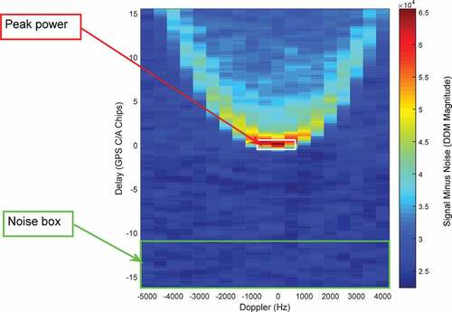
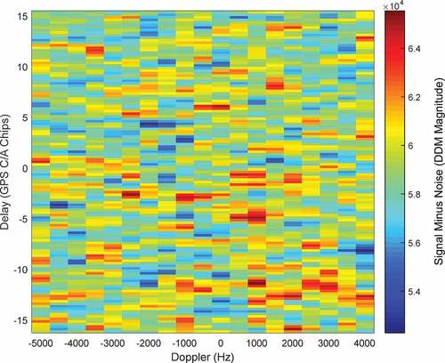
Due to system noise and sea ice effects, the DDM from SGR-ReSI does not always exhibit the “horseshoe” shape, as shown in Figure 1, but a garbled situation as shown in Figure 2. In Figure 2, the characteristic horseshoe shape is lost in the noise. Therefore, quality control (QC) is required to remove these inferior quality DDMs before wind speed retrieval. Comparing Figures 1 and 2, the fluctuations are relatively small in the DDM noise box, which show the characteristic “horseshoe” shape in Figure 1, while the fluctuations of noisy DDMs are large in Figure 2. These noisy DDMs usually exist in the observables at high incident angles and low AGSP. Therefore, the DDMs withincident angles larger than 35° and AGSPs less than 0 dB are considered for further analysis. Besides, the DDMs with the difference between the maximum and minimum values greater than 10,000 in the noise box are also removed.

Figure 2. An example of a noisy DDM retrieved by the SGR-ReSi instrument.

To balance the accuracy and spatial coverage, the process of wind speed retrieval is as follows. First, DDM datasets are divided into two parts: high SNR (>0 dB) and low SNR (>−10 dB and ≤0 dB). Then, QC is applied to filter out poor-quality data both at high and low SNR datasets. After correcting the receiver antenna gain effects and GNSS-R geometry effects, the remaining datasets are divided into different parts according to different GPS blocks to develop GMF and to retrieve wind speed. Finally, the influence of Hs on SNR observables is analyzed.

3. Dataset

3.1. UK TechDemoSat-1

In this study, the datasets from TDS-1, ASCAT and ECMWF are used. TDS-1 can process GPS reflected signals into DDMs, from which ocean roughness and wind field can be retrieved. TDS-1 has been operated in two modes, including Unmonitored Automatic Gain Control (UAGC) (from September 2014 to April 2015) and Fixed Gain Mode (FGM) (After May 2015). Since the receiver absolute powers operated in UAGC were unknown, the receiver operated in FGM is more effective for calibration purposes. Both modes can generate DDMs, which belong to level 1b data in the TDS-1 datasets. Besides the L1b dataset, TDS-1 datasets also provide levels 0 and 2 datasets, including raw data and wind speeds (Jales and Unwin 2016). The level 1b data, from May 2015 to May 2016, is used in this study. In order to avoid the influence of sea ice, the ocean data at latitudes between ±55° are used. The datasets are available at http://merrbys.co.uk/.

3.2. Advanced scatterometer

The ASCAT, operating at a frequency of 5.255 GHz (C-band), is one of the instruments using vertically polarized antennas. As an aperture radar, ASCAT onboard the Meteorological Operational (Metop) polar satellites, Metop-A, Metop-B, and Metop-C, have been launched on autumn of 2006, 2012, 2018, respectively, by the European Space Agency (ESA). The three missions have been operated by the European organization for the Exploitation of Meteorological Satellites (EUMETSAT). It generates radar beams on both sides of the satellite ground track, which illuminates as wide as 550 km swaths (separated by about 700 km). As the satellite moves along its orbit, each swath provides measurements of radar backscatter from the ocean surface on a 25 km or 12.5 km grid, which is divided into 21 or 41 so-called wind vector cells (WVCs). In this way, ASCAT provides 25-km and 12.5-km products for the effective swath width to 525 km (21 × 25) or 512.5 km (41 × 12.5), respectively. Compared with buoys data, the RMSE of ASCAT wind speed data is less than 1.72 m/s (Bentamy 2008). The ASCAT data are available from the Physical Oceanography Distributed Active Archive Center (https://podaac.jpl.nasa.gov/). In this study, the ASCAT dataset is matched with the TDS-1 dataset applying the following criteria: time ≤30 minutes and distance ≤25 km in space.

3.3. ECMWF

For each hour a day, the fifth-generation ECMWF atmospheric reanalysis of the global climate so-called ERA5 provides wind speed, the Hs, and pressure levels. Reanalysis combines modeled data with observations from across the world to a globally complete and consistent dataset by using the physics laws. The ECMWF dataset can be downloaded from the European Center for Medium-Range Weather Forecasts (https://www.ecmwf.int/). In this study, the wind speed and Hs from ERA5 are used for analysis. The ERA5 data is matched with the TDS-1 dataset applying the following criteria: time ≤30 minutes and latitude and longitude ≤0.25°.

4. Results and discussions

4.1. GMF and wind speed retrieval results against ASCAT/ECMWF winds at high SNR

As mentioned above, the data at high SNR with SNRs >0 dB are used to develop GMF. Figures 3 and 5 show SNRc against ASCAT/ECMWF wind speed matchup dataset randomly used for training (75% of samples) all GPS blocks and each GPS block as well as GMF. Outliers are removed according to the three sigma rules. Figures 4 and 6

Figure 3. TDS-1 SNRc with SNRs >0 dB and the corresponding ASCAT wind speeds for the training dataset (75% of samples) of all GPS blocks in (a) and each GPS block in (b)–(f). The white curve represents GMF. The form of GMF is $U_{10}=\mathit{A}{e}^{\mathit{xB}}$, where $\mathit{x}$ represents SNRc.

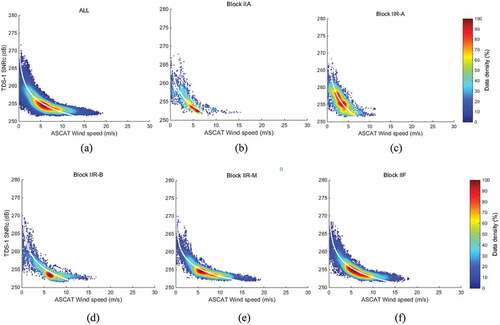
Figure 4. (a)–(f) The wind speed retrievals of TDS-1 versus collocated ASCAT wind speed for the remaining test dataset (25% of samples) of all GPS blocks and each GPS block. The black line represents TDS-1 wind speed equal to ASCAT wind speed.

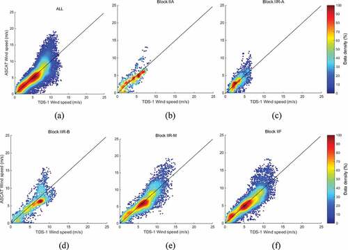
Figure 5. TDS-1 SNRc with SNRs >0 dB and the corresponding ECMWF wind speeds for the training dataset (75% of samples) of all GPS blocks in (a) and each GPS block in (b)–(f). The white curve represents GMF. The form of GMF is $U_{10}=\mathit{A}{e}^{\mathit{xB}}$, where $\mathit{x}$ represents SNRc.

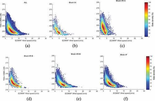
Figure 6. The wind speed retrievals of TDS-1 and the corresponding ECMWF wind speed for the remaining test dataset (25% of samples) of all GPS blocks in (a) and each GPS block in (b)–(f). The black line represents TDS-1 wind speed equal to ECMWF wind speed.

show the wind speed retrievals against ASCAT/ECMWF winds for the remaining independent test subset (25% of samples) for all GPS blocks and each GPS block. Similar trends of GMFs and wind speed results are found in each GPS block. For further analysis, Table 1 shows the results against ASCAT and ECMWF at high SNRs.

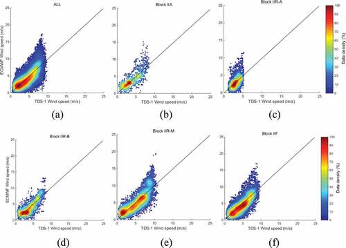
Table 1. Performance of each GPS block against ASCAT and ECMWF at high SNR

	GPS block	All	Block IIA	Block IIR-A	Block IIR-B	Block IIR-M	Block IIF
ASCAT	RMSE (m/s)	2.19	1.48	1.47	2.01	1.95	1.93
	Correlation coefficient	0.79	0.78	0.70	0.80	0.85	0.84
	Samples	67825	3477	8035	7182	20036	27356
ECMWF	RMSE (m/s)	1.88	1.69	1.51	1.53	1.86	1.72
	Correlation coefficient	0.72	0.76	0.49	0.76	0.79	0.76
	Samples	110265	5030	16979	10826	27390	47291

In general, although the winds from ECMWF especially at low winds are more discrete than ASCAT for all GPS blocks, the GMF trends and the wind speed retrieval results versus ASCAT and ECMWF are similar. It is worth mentioning that most of the on-orbit GPS satellites are the types of Block IIR and Block IIF, thus having more training or test samples for these two kinds of blocks. Compared with ASCAT and ECMWF, their accuracy values of wind speed retrieval are 2.19 m/s and 1.88 m/s, respectively, when all TDS data are processed without distinguishing GPS block types. However, if the TDS data are separately processed and used to develop wind GMF through different blocks, both the accuracy and correlation coefficient can be improved to some extent. Block IIA and block IIR-A show smaller RMSEs of 1.48 m/s and 1.47 m/s for ASCAT and 1.69 m/s and 1.51 m/s for ECMWF, which may be attributed to the following two reasons. On the one hand, the wind speeds of blocks IIA and IIR-A are mostly concentrated at lower speed (<15 m/s). On the other hand, the numbers of available samples of these two block types are much smaller than the other blocks.

4.2. GMF and wind speed retrieval results against ASCAT/ECMWF winds at low SNR

Likewise, the data at low SNR with 10 dB < SNR ≤ 0 dB are used to develop GMF. Figures 7 and 9 show the SNRc against ASCAT/ECMWF wind speed matchup dataset randomly used for training (75% of samples) all GPS blocks and each GPS block. Different from the GMF form at high SNR, the GMF form at low SNR is a linear model. Figures 8 and 10 show the wind speed retrievals against ASCAT/ECMWF winds for the remaining independent test subset (25% of samples) of all GPS blocks and each GPS block

Figure 7. TDS-1 SNR_c with SNRs ≤ 0 dB and SNRs > −10 dB and the corresponding ASCAT wind speeds for the training dataset (75% of samples) of all GPS blocks in (a) and each GPS block in (b)–(f). The white curve represents GMF. The form of GMF is $U_{10}=\mathit{Ax}$, where $\mathit{x}$ represents SNRc.

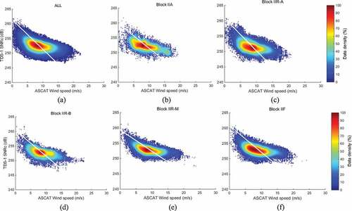
Figure 8. The wind speed retrievals of TDS-1 and the corresponding ASCAT wind speed for the remaining test dataset (25% of samples) of all GPS blocks in (a) and each GPS block in (b)–(f). The black line represents TDS-1 wind speed equal to ASCAT wind speed.

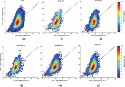
Figure 9. TDS-1 SNR_c with SNRs ≤ 0 dB and SNRs > −10 dB of the corresponding ECMWF wind speeds for the training dataset (75% of samples) of all GPS blocks in (a) and each GPS block in (b)–(f). The white curve represents GMF. The form of GMF is $U_{10}=\mathit{Ax}$, where $\mathit{x}$ represents SNRc.

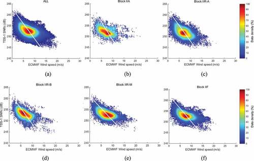
Figure 10. The wind speed retrievals of TDS-1 and the corresponding ECMWF wind speeds for the remaining test dataset (25% of samples) of all GPS blocks in (a) and each GPS block in (b)–(f). The black line represents that TDS-1 wind speed is equal to ECMWF wind speed.

. Table 2 shows the results against ASCAT and ECMWF at low SNR.

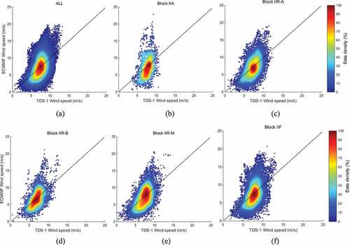
Table 2. Performance of each GPS block against ASCAT and ECMWF at low SNR

	GPS block	All	Block IIA	Block IIR-A	Block IIR-B	Block IIR-M	Block IIF
ASCAT	RMSE (m/s)	3.13	3.09	2.92	3.04	2.96	3.03
	Correlation coefficient	0.50	0.57	0.52	0.56	0.59	0.52
	Samples	202344	18179	56754	24124	45807	54930
ECMWF	RMSE (m/s)	2.74	3.14	2.52	2.49	2.54	2.82
	Correlation coefficient	0.49	0.36	0.53	0.54	0.54	0.48
	Samples	197612	11245	54300	21459	42698	64855

Note that the GMF in this section is Linear model. The reason for choosing linear model is that the Linear model has better performance with smaller RMSE and higher correlation coefficient compared with other functions, e.g. exponential and power Law. In addition, GMFs from low SNR do not cross the center point of the contour like high SNR. The reason is that if the GMF crosses the center point, the slope of the GMF at high wind will be very large, which will lead to a large wind speed range corresponding to one SNRc and severely decrease the wind speed retrieval accuracy. Therefore, Figures 7 and 9 show GMFs corresponding to the minimum RMSEs and maximum correlation coefficients. Compared with ASCAT and ECMWF, the accuracy values of wind speed retrieval are 3.13 m/s and 2.74 m/s, respectively, when all TDS data are processed without distinguishing GPS block types. The performance at low SNR data is poorer than the performance at high SNR due to the high wind speed data at low SNR larger than that of high SNR. On the other hand, it also demonstrates that the quality of SNR data is better than that of low SNR data. Since there are many winds (>13 m/s) that deviate from the GMF, the RMSE of block IIA is larger than that of all blocks in ECMWF, thus leading to poor GMF and small correlation coefficients. However, the samples of low SNR with 202344 and 197612 for ASCAT and ECMWF, respectively, are larger than the samples of high SNR, 67825 and 110265 for ASCAT and ECMWF, respectively, which can maintain large spatial coverage. Furthermore, similar to high SNR, if the TDS data are separately processed and used to develop wind GMF through different blocks, both the accuracy and correlation coefficient can be improved at low SNR. In addition, our analysis was done with TDS, which only has one antenna and one observatory limited publicly available characterizations, specifically related to their actual transmit power, antenna patterns, and attitude. This calibration issue may be attributed to the unknown GPS transmit powers from different PRNs, not correctly accounted for in the bistatic radar equation. Because TDS-1 has limited publicly available characterizations specifically related to their actual transmit power and antenna patterns, we can only analyze the influence of different GPS blocks on wind speed retrieval.

5. Observable versus sea state

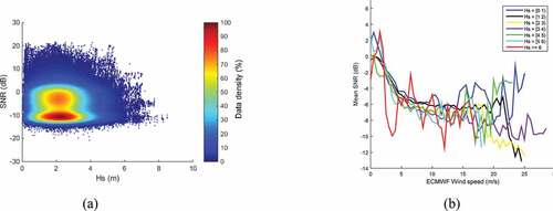
As described in (Soisuvarn et al. 2016), the DDM is affected not only by wind field but also by the sea state such as swell. Therefore, it is worth investigating the relationship between observables and other parameters other than wind. Here, we consider the sensitivity of observables to Hs. Figure 11(a) shows the relationship between Hs and SNR. As shown in Figure 11(a), there are a lot of lower SNRs (<−10 dB) between 0 m and 4 m of Hs. Thus, it is necessary to use QC to filter out poor DDMs. To more intuitively see the effect of Hs on the observables, Figure 11(b) shows the relationship between ECMWF wind speed and mean SNR at different Hs. As the wind speed increases, the SNR decreases. When Hs is greater than 6 m, the SNR changes drastically due to the limited number of samples

Figure 11. (a) Relationship between Hs and SNR collocated with ECMWF. (b) Relationship between ECMWF wind speed and mean SNR.

.

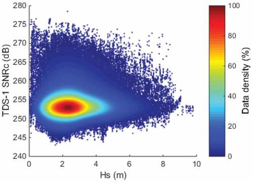
Since SNRc is applied to develop GMF, it is worth to analyze whether the SNRc is influenced by Hs. Figure 12 shows the relationship between ECMWF Hs and SNRc. In general, the SNRc decreased with Hs. Hs is mainly distributed in 0–4 m, and the SNRc are clustered around 252.5 dB. There is no obvious linear or nonlinear relationship between SNRc and Hs in the concentrated part. However, adding a Hs for the corrected factor into GMF into a discrete part may contribute a better wind speed retrieval, which needs further study.

Figure 12. Relationship between ECMWF Hs and SNRc.

6. Conclusions

In this paper, the TDS-1 GNSS reflectometry wind geophysical model function response to GPS block was proposed. First, the method of wind speed retrieval from DDMs was presented. To balance the accuracy and spatial coverage, this method divided DDM datasets into two parts: high SNR (>0 dB) and low SNR (>−10 dB and ≤0 dB) to develop wind GMF. During the progress, the observable was accounted for by the receiver antenna gain effects and GNSS-R geometry effects. After correcting the above elements, the sensitivity of the corrected SNR (SNRc) to GPS block was investigated. Then, the SNRc was used to develop GMF by using different GPS blocks. Finally, the influence of Hs on SNR observables is analyzed.

The results show that although the winds from ECMWF are more discrete than ASCAT for all GPS blocks especially at low winds, the GMF trends and the wind speed retrieval results versus ASCAT and ECMWF are similar. The block types have impacts on wind GMF and the use of a prior GPS block can contribute to a better wind speed retrieval at both high and low SNR. Compared with ASCAT, the RMSE values of wind speed retrieval at high and low SNR are 2.19 m/s and 3.13 m/s, respectively, when all TDS-1 data are processed without distinguish GPS block types. However, if the TDS-1 data are separately processed and used to develop wind GMF through different blocks, both the accuracy and correlation coefficient can be improved to some extent. Although the performance of low SNR is poorer than high SNR, the samples of low SNR is larger than high SNR, which can maintain large spatial coverage.

Acknowledgments

The authors would like to thank the TDS-1 team at Surrey Satellite Technology Ltd. for providing TDS-1 data as well as the team associated with ASCAT and ECMWF.

Disclosure statement

No potential conflict of interest was reported by the author(s).

Data availability statement

The TDS-1 dataset is available at http://merrbys.co.uk/. The ASCAT dataset is available at https://podaac.jpl.nasa.gov/. The ECMWF dataset is available at https://www.ecmwf.int/.

Additional information

Funding

This work is supported by the Funds for Creative Research Groups of China [Grant no. 41721003] and the National Natural Science Foundation of China [Grant nos. 41825009 and 41774034].

Notes on contributors

Fade Chen

Fade Chen is currently a PhD candidate at Wuhan University. He completed his B.Sc. degree in 2015 and his master’s degree in 2018 at Guilin University of Technology. His current research focuses on GNSS Reflectometry.

Xiaohong Zhang

Xiaohong Zhang is currently a professor at Wuhan University. He obtained his B.Sc., M.Sc. and Ph.D. degrees with distinction in geodesy and engineering surveying at Wuhan University in 1997, 1999 and 2002, respectively. His main research interests include PPP, GNSS/INS navigation, and their applications in geoscience and engineering.

Fei Guo

Fei Guo is currently a professor at Wuhan University. He received his B.Sc. degree in survey engineering from Nanjing Forestry University in 2007. He obtained his M.Sc., and PhD degrees with distinction in geodesy from Wuhan University in 2009 and 2013, respectively. His current research mainly focuses on precise GNSS positioning and its application in geoscience.

Jiazhu Zheng

Jiazhu Zheng is currently an associate professor at Nanjing Forestry University. He received his PhD degrees in Geodesy in Hohai University. His research interests include indoor positioning and remote sensing.

Yang Nan

Yang Nan is currently a PhD candidate at Wuhan University. His current research focuses on GNSS Reflectometry.

Mohamed Freeshah

Mohamed Freeshah is currently a post-doctoral at Wuhan University. He received a Bachelor of Engineering in Surveying from Benha University, Egypt in 2010; Scholarship from Academy of Scientific Research and Technology for funding MSc, Egypt in 2013. Master of Engineering in Geodesy and Surveying from Benha University, Egypt in 2016. He received his PhD degree in 2021 in Wuhan University. His main research interests include GNSS and ionospheric disturbances.

References

- Alonso-Arroyo, A., V. U. Zavorotny, and A. Camps. 2016. “Sea Ice Detection Using GNSS-R Data from UK TDS-1.” In IEEE International Geoscience and Remote Sensing Symposium (IGARSS). Beijing, November 3.
- Asgarimehr, M., J. Wickert, and S. Reich. 2018. “TDS-1 GNSS Reflectometry: Development and Validation of Forward Scattering Winds.” IEEE Journal of Selected Topics in Applied Earth Observations & Remote Sensing 11 (11): 4534–4541. doi:10.1109/JSTARS.2018.2873241.
- Auber, J. C., A. Bibaut, and J. M. Rigal. 1994. “Characterization of Multipath on Land and Sea at GPS Frequencies.” In The 7th International Technical Meeting of the Satellite Division of The Institute of Navigation (ION GPS 1994). Salt Lake City, September 20–23.
- Balasubramaniam, R., and C. Ruf. 2020. “Characterization of Rain Impact on L-Band GNSS-R Ocean Surface Measurements.” Remote Sensing of Environment 239 (15): 111607. doi:10.1016/j.rse.2019.111607.
- Bentamy, A. 2008. “Characterization of ASCAT Measurements Based on Buoy and QuikSCAT Wind Vector Observations.” Ocean Science Discussions 5 (1): 77–101.
- Camps, A., H. Park, M. Pablos, G. Foti, C. P. Gommenginger, P. W. Liu, and J. Judge. 2016. “Sensitivity of GNSS-R Spaceborne Observations to Soil Moisture and Vegetation.” IEEE Journal of Selected Topics in Applied Earth Observations & Remote Sensing 9 (10): 4730–4742. doi:10.1109/JSTARS.2016.2588467.
- Cardellach, E., F. Fabra, O. Nogues-Correig, S. Oliveras, S Ribó, and A. Rius. 2011. “GNSS-R Ground-based and Airborne Campaigns for Ocean, Land, Ice, and Snow Techniques: Application to the GOLD-RTR Data Sets.” Radio Science 46 (6): 1–16. doi:10.1029/2011RS004683.
- Chew, C., and E. Small. 2020. “Description of the UCAR/CU Soil Moisture Product.” Remote Sensing 12 (10): 1558. doi:10.3390/rs12101558.
- Chew, C., R. Shah, C. Zuffada, G. Hajj, D. Masters, and A. J. Mannucci. 2016. “Demonstrating Soil Moisture Remote Sensing with Observations from the UK TechDemoSat-1 Satellite Mission.” Geophysical Research Letters 43 (7): 3317–3324. doi:10.1002/2016GL068189.
- Clarizia, M. P., C. P. Gommenginger, S. T. Gleason, M. A. Srokosz, and M. D. Bisceglie. 2009. “Analysis of GNSS-R delay-Doppler Maps from the UK-DMC Satellite over the Ocean.” Geophysical Research Letters 36 (2): L02608. doi:10.1029/2008GL036292.
- Clarizia, M. P., C. S. Ruf, P. Jales, and C. Gommenginger. 2014. “Spaceborne GNSS-R Minimum Variance Wind Speed Estimator.” IEEE Transactions on Geoscience & Remote Sensing 52 (11): 6829–6843. doi:10.1109/TGRS.2014.2303831.
- Foti, G., C. Gommenginger, M. Unwin, P. Jales, J. Tye, and J. Roselló. 2017. “An Assessment of Non-geophysical Effects in Spaceborne GNSS Reflectometry Data from the UK TechDemoSat-1 Mission.” IEEE Journal of Selected Topics in Applied Earth Observations & Remote Sensing 10 (7): 3418–3429. doi:10.1109/JSTARS.2017.2674305.
- Foti, G., C. Gommenginger, P. Jales, M Unwin, and J. Roselló. 2015. “Spaceborne GNSS-Reflectometry for Ocean Winds: First Results from the UK TechDemoSat-1 Mission: Spaceborne GNSS-R: First TDS-1 Results.” Geophysical Research Letters 42 (13): 5435–5441. doi:10.1002/2015GL064204.
- Garrison, J. L., A. Komjathy, V. U. Zavorotny, and S. J. Katzberg. 2002. “Wind Speed Measurement Using Forward Scattered GPS Signals.” IEEE Transactions on Geoscience & Remote Sensing 40 (1): 50–65. doi:10.1109/36.981349.
- Garrison, J. L., S. J. Katzberg, and M. I. Hill. 1998. “Effect of Sea Roughness on Bistatically Scattered Range Coded Signals from the Global Positioning System.” Geophysical Research Letters 25 (13): 2257–2260. doi:10.1029/98GL51615.
- Gleason, S. T. 2006. “Remote Sensing of Ocean, Ice and Land Surfaces Using Bistatically Scattered GNSS Signals from Low Earth Orbit.” Ph.D diss., University of Surrey.
- Gleason, S. T., S. Hodgart, Y. Sun, C. Gommenginger, and M Unwin. 2005. “Detection and Processing of Bistatically Reflected GPS Signals from Low Earth Orbit for the Purpose of Ocean Remote Sensing.” IEEE Transactions on Geoscience & Remote Sensing 43 (6): 1229–1241. doi:10.1109/TGRS.2005.845643.
- Gleason, S. T. 2010. “Towards Sea Ice Remote Sensing with Space Detected GPS Signals: Demonstration of Technical Feasibility and Initial Consistency Check Using Low Resolution Sea Ice Information.” Remote Sensing 2 (8): 2017–2039. doi:10.3390/rs2082017.
- Hall, C., and R. Cordey. 1988. “Multistatic Scatterometry.” In International Geoscience and Remote Sensing Symposium, ‘Remote Sensing: Moving Toward the 21st Century’. Edinburgh, September 12–16.
- Jales, P., and M. Unwin. 2016. MERRByS Product Manual: GNSS-Reflectometry on TDS-1 with the SGR-ReSI. Guildford: Surrey Satellite Technology Limited.
- Komjathy, A., M. Armatys, D. Masters, P. Axelrad, V. Zavorotny, and S. Katzberg. 2004. “Retrieval of Ocean Surface Wind Speed and Wind Direction Using Reflected GPS Signals.” Journal of Atmospheric and Oceanic Technology 21 (3): 515–526. doi:10.1175/1520-0426(2004)021<0515:ROOSWS>2.0.CO;2.
- Li, C., and W. Huang. 2014. “An Algorithm for Sea-Surface Wind Field Retrieval from GNSS-R Delay-Doppler Map.” IEEE Geoscience and Remote Sensing Letters 11 (12): 2110–2114. doi:10.1109/LGRS.2014.2320852.
- Lin, W., M. Portabella, G. Foti, A. Stoffelen, C. Gommengiger, and Y. He. 2019. “Toward the Generation of a Wind Geophysical Model Function for Spaceborne GNSS-R.” IEEE Transactions on Geoscience & Remote Sensing 57 (12): 655–666. doi:10.1109/TGRS.2018.2859191.
- Liu, Y., W. Jiang, and X. Zhou. 2008. “Ocean Loading Tides Corrections of GPS Stations in Antarctica.” Geo-spatial Information Science 11 (2): 148–151. doi:10.1007/s11806-008-0060-5.
- Llaveria, D., J. F. Munoz-Martin, C. Herbert, M. Pablos, and A. Camps. 2021. “Sea Ice Concentration and Sea Ice Extent Mapping with L-Band Microwave Radiometry and GNSS-R Data from the FFSCat Mission Using Neural Networks.” Remote Sensing 13 (6): 1139. doi:10.3390/rs13061139.
- Lowe, S. T., C. Zuffada, Y. Chao, P. Kroger, L. E. Young, and J. L. Labrecque. 2002. “5-cm-precision Aircraft Ocean Altimetry Using GPS Reflections.” Geophysical Research Letters 29 (10): 13-1–13-4. doi:10.1029/2002GL014759.
- Martín-Neira, M. 1993. “A Passive Reflectometry and Interferometry System (PARIS): Application to Ocean Altimetry.” ESA Journal 17 (4): 331–355.
- Nogues-Correig, O., S. Ribo, J. C. Arco, E. Cardellach, and M. Martín-Neira. 2010. “The Proof of Concept for 3-cm Altimetry Using the Paris Interferometric Technique.” In International Geoscience and Remote Sensing Symposium (IGARSS). Honolulu, July 25–30.
- Portabella, M., A. Stoffelen, W. Lin, A. Turiel, A. Verhoef, J. Verspeek, J. Ballabrera-Poy, et al. 2012. “Rain Effects on ASCAT-retrieved Winds: Toward an Improved Quality Control.” IEEE Transactions on Geoscience & Remote Sensing 50 (7): 2495–2506. DOI:10.1109/TGRS.2012.2185933.
- Rodriguez-Alvarez, N., D. M. Akos, V. U. Zavorotny, J. A. Smith, A. Camps, and C. W. Fairall. 2013. “Airborne GNSS-R Wind Retrievals Using delay–Doppler Maps.” IEEE Transactions on Geoscience & Remote Sensing 51 (1): 626–641. doi:10.1109/TGRS.2012.2196437.
- Ruf, C. S., S. Gleason, Z. Jelenak, S. Katzberg, A. Ridley, R. Rose, J. Scherrer, and V. Zavorotny. 2012. “The CYGNSS Nanosatellite Constellation Hurricane Mission.” In IEEE Geoscience & Remote Sensing Symposium, Munich, Germany, 22–27 July 2012, 214–216.
- Ruf, C., D. J. Posselt, S. Majumdar, S. Gleason, M. P. Clarizia, D. Starkenburg, D. Provost, et al. 2016. CYGNSS Handbook. Ann Arbor: Michigan Publishing.
- Ruffini, N. G., F. Soulat, M. Caparrini, O. Germain, and M. Martín-Neira. 2004. “The Eddy Experiment: Accurate GNSS-R Ocean Altimetry from Low Altitude Aircraft.” Geophysical Research Letters 31 (12): L12306. doi:10.1029/2004GL019994.
- Said, F., Z. Jelenak, P. S. Chang, and S. Soisuvarn. 2019. “An Assessment of CYGNSS Normalized Bistatic Radar Cross Section Calibration.” IEEE Journal of Selected Topics in Applied Earth Observations & Remote Sensing 12 (1): 50–65. doi:10.1109/JSTARS.2018.2849323.
- Soisuvarn, S., Z. Jelenak, F. Said, P. S. Chang, and A. Egido. 2016. “The GNSS Reflectometry Response to the Ocean Surface Winds and Waves.” IEEE Journal of Selected Topics in Applied Earth Observations & Remote Sensing 9 (10): 4678–4699. doi:10.1109/JSTARS.2016.2602703.
- Stiles, B. W., and S. H. Yueh. 2002. “Impact of Rain on Spaceborne Ku-band Wind Scatterometer Data.” IEEE Transactions on Geoscience & Remote Sensing 40 (9): 1973–1983. doi:10.1109/TGRS.2002.803846.
- Tye, J., P. Jales, M. Unwin, and C. Underwood. 2016. “The First Application of Stare Processing to Retrieve Mean Square Slope Using the SGR-ReSI GNSS-R Experiment on TDS-1.” IEEE Journal of Selected Topics in Applied Earth Observations & Remote Sensing 9 (10): 4669–4677. doi:10.1109/JSTARS.2016.2542348.
- Unwin, M., P. Jales, J. Tye, C. Gommenginger, G. Foti, and J. Rosello. 2016. “Spaceborne GNSS-reflectometry on TechDemoSat-1: Early Mission Operations and Exploitation.” IEEE Journal of Selected Topics in Applied Earth Observations & Remote Sensing 9 (10): 4525–4539. doi:10.1109/JSTARS.2016.2603846.
- Wang, F., D. Yang, B. Zhang, W. Li, and J. Darrozes. 2016. “Wind Speed Retrieval Using Coastal Ocean-scattered GNSS Signals.” IEEE Journal of Selected Topics in Applied Earth Observations & Remote Sensing 9 (11): 5272–5283. doi:10.1109/JSTARS.2016.2611598.
- Yan, Q., and W. Huang. 2016. “Spaceborne GNSS-R Sea Ice Detection Using Delay-Doppler Maps: First Results from the UK TechDemoSat-1 Mission.” IEEE Journal of Selected Topics in Applied Earth Observations & Remote Sensing 9 (11): 4795–4801. doi:10.1109/JSTARS.2016.2582690.
- Yan, Q., W. Huang, S. Jin, and Y. Jia. 2020. “Pan-tropical Soil Moisture Mapping Based on a Three-layer Model from CYGNSS GNSS-R Data.” Remote Sensing of Environment 247: 111944. doi:10.1016/j.rse.2020.111944.
- Zhou, Z., Y. Fu, Z. Xue, and H. Cui. 2006. “Remote Sensing of Sea Surface Wind of Hurricane Michael by GPS Reflected Signals.” Geo-spatial Information Science 9 (1): 24–31. doi:10.1007/BF02826684.