A novel method for road network mining from floating car data

ABSTRACT

Vehicles have been increasingly equipped with GPS receivers to record their trajectories, which we call floating car data. Compared with other data sources, these data are characterized by low cost, wide coverage, and rapid updating. The data have become an important source for road network extraction. In this paper, we propose a novel approach for mining road networks from floating car data. First, a Gaussian model is used to transform the data into bitmap, and the Otsu algorithm is utilized to detect road intersections. Then, a clothoid-based method is used to resample the GPS points to improve the clustering accuracy, and the data are clustered based on a distance-direction algorithm. Last, road centerlines are extracted with a weighted least squares algorithm. We report on experiments that were conducted on floating car data from Wuhan, China. To conclude, existing methods are compared with our method to prove that the proposed method is practical and effective.

KEYWORDS:

• GPS trajectory
• floating car data
• road intersection extraction
• data clustering

1. Introduction

A road map is a compilation of roads and transport links (“Roadmap” 2021). It plays an important role in many aspects of our lives, such as navigation, urban management (Wu, Gui, and Yang 2020) and Location-Based Services (LBSs) (Huang and Wang 2020; Zuo, Liu, and Fu 2020). Along with the development of LBSs, demands for map accuracy are increasingly stringent. However, road construction is a frequent activity, and roads are quickly updated. For instance, in China, the total length of highways was $3.73\times {10}^6$ km in 2008, and grew to $5.2\times {10}^6$ km in 2020. Therefore, the road map needs to keep up to date to follow the increase in road construction. There are two main sources of update data: (1) road information extracted from aerial images (Yuan and Cheriyadat 2016; Karaduman, Cinar, and Eren 2019; Zhang et al. 2019; Wang, Hou, and Ren 2017) and (2) road information collected by professionally operated probe cars (Gwon et al. 2017; Jo and Sunwoo 2014; Massow et al. 2016). The first source consists of high-resolution satellite images that are processed with a shape classification algorithm to estimate the boundaries of roads. Aerial images are an important source of road map updates. However, it is costly to acquire suitable satellite images. The second source requires probe cars equipped with on-board sensors such as Real-Time Kinematic (RTK) GPS, Post-Processing Kinematic (PPK) devices, and laser scanners to collect road information (Sester 2020). The accuracy of the resulting maps is higher than that of the first method. However, in addition to the high cost of on-board sensors, this method is a labor-intensive way to collect road information.

Considering the limitations of the two mentioned methods, some researchers have proposed extracting road maps from floating car data (Wang et al. 2015; Zheng and Zhu 2019; Fang et al. 2016). As the cost of GPS and communication technologies has decreased this year, many vehicles are equipped with a GPS to record trace data. In contrast to aerial images, floating car data is accessible, has wide coverage, is available in large amounts, and is quickly updated. However, the accuracy of GPS data can only reach 5 m – 30 m due to signal interruptions and multipath transmission. The large set of trajectories can compensate for the shortcomings in accuracy, but the accuracy makes it difficult to mine road networks from these data. In this paper, we propose a novel method of extracting road maps from floating car data.

In general, the main contributions of this paper are as follows:

1. An Otsu-based background segmentation algorithm is introduced to detect road intersections;

2. A gamma-correction-based spatiotemporal prediction algorithm is utilized to increase the accuracy of intersection detection;

3. A clothoid curve is used to resample the GPS data, and the distance and direction similarity are combined to cluster the data.

2. Related work

There are three main steps to mining road maps from floating car data: intersection detection, data clustering, and centerline extraction of roads from the clustering data. As an important component of roads, the structure of intersection is more complex than road segments. Therefore, intersection detection is the first step in generating a road network from floating car data. Then, it is necessary to cluster the trajectories together that belong to the same road. Finally, to describing the shape of road, centerline extraction is essential.

Road intersection extraction is one of the most important and difficult steps in road network mining. Some studies have identified road intersections and segments from the angle and distance of their trajectory (Fathi and Krumm 2010; Yang et al. 2018). In addition, the speed threshold combined with direction changes was used to detect intersections (Chen et al. 2020). In reference (Deng et al. 2018), a local G* statistic was introduced to detect GPS points with large turning angles. Wang et al. (2015) determined intersection boundaries by analyzing conflict points that have large intersection angles. The turning angle is an important feature for detecting intersections from trajectory data in the studies mentioned above. However, the heading angles of GPS points are inaccurate because of signal interruptions and multipath transmission.

The methods of clustering include (1) clustering based on the density of GPS points (Biagioni and Eriksson 2012; Li et al. 2018) and (2) clustering based on the direction and distance features of GPS traces (Tang et al. 2016; Deng et al. 2018; Li et al. 2012; Liu et al. 2012). The kernel density method is the most commonly used way to build the probability function of similar GPS points for clustering (Biagioni and Eriksson 2012). The Delaunay triangulation network is also utilized to cluster the GPS points (Li et al. 2018). However, this density-based method cannot cluster points correctly in road intersections.

Clustering methods based on the direction and distance of traces are widely used and work on most occasions. Tang et al. (2016) presented a region growing clustering method to cluster GPS trajectories that used the vertical and angular differences of trajectory vectors and assigned different weighting values to the vertical distance and angle to calculate trajectory similarity. Deng et al. (2018) combined the longest common sub-track with a distance-direction function to calculate the total similarity of adjacent tracks. First, the shape similarity of two adjacent tracks was measured by calculating the ratio of the longest matched sub-trace between two associated trajectories. Then, a distance-direction function was used to compute the heading direction similarity. The overall similarity was measured by combining the two steps. Based on the position and direction components of GPS traces, Li et al. (2012) added a semantic relationship to classify GPS points. In addition, Liu et al. (2012)further optimized the distance and direction-based method. The orientation similarity and geographical distance were used first to perform basic clustering. Then, a clustering refinement method was proposed. The main concept of the refinement method was to calculate backbone curves to represent roads first and then group the closest samples to a smaller cluster. The algorithms mentioned above can work effectively in some instances, but they fail on complex roads.

Extracting the centerline of a road from floating car data is an important step. Various algorithms have been proposed to accurately describe the geometrical shape of roads. Some researches converted floating car data into bitmaps and used a grayscale map skeletonization method to thin and prune the data to generate its centerline (Shi, Shen, and Liu 2009; Biagioni and Eriksson 2012; Chen and Cheng 2008). This method can extract centerlines successfully when the density of GPS points remains moderate. However, it failed when the density of points became very large or small. Li et al. (2012) and Bruntrup et al. (2005) used an incremental method to generate road networks from GPS data. They grouped the traces that belonged to the same road first and utilized an incremental approach to generate the centerline. This method needs to match all trajectories and modify the centerline step by step, causing low efficiency. Some studies introduced a Gaussian mixture model to extract the number and location of lanes from GPS data (Chen and Krumm 2010; Guo, Iwamura, and Koga 2007), assuming that these data follow a normal distribution. However, this method is better suited to data with high accuracy and obtained in a controlled environment (Winden, Biljecki, and Van Der Spek 2016; Ahmed et al. 2015). In addition, Cao and Krumm (2009) proposed a point-based physical attraction model to generate the centerline. It was assumed that there are two types of forces acting on a GPS point. One is the total gravitation force from the neighboring points. Another is the spring force to keep a point in its original position. The efficiency of this method is low and is invalid when the density of GPS points is high.

In contrast to these methods, in this paper, the Otsu algorithm, which is often used in computer vision to segment foreground and background, is adopted to detect road intersections. Furthermore, a clothoid curve is utilized to resample the floating car data, and a direction-distance clustering algorithm is used to cluster the data to group similar trajectories together. Finally, the centerline of the road is extracted with a weighted least squares algorithm.

3. Method

In this section, we elaborate on our methods, which include road intersection detection and data clustering. First, we convert the GPS data to raster data with a Gaussian model and detect road intersections with the Otsu algorithm. Then, we use a clothoid-based method to resample the trajectories and calculate their distance and direction similarity to cluster the similar ones together. Finally, we describe a piecewise weighted least square fitting method that extracts the centerline of the clustered data and builds a road network that describes the topology and geometry of the roads.

3.1. Problem statement

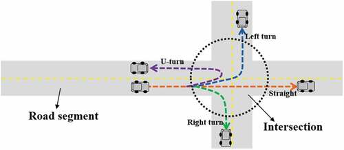
A complete road can be separated into road segments and intersections, as shown in Figure 1. Road intersection detection is critical to mining road networks from floating car data. A road intersection is a junction where more than two roads meet or cross. Compared with a road segment, intersections are more complex because they may include a left-turn lane, right-turn lane, straight lane, and U-turn lane as represented in Figure 1. To exactly represent the road shape, the road intersection cannot be described by a single point. Therefore, clustering is necessary to group similar GPS trajectories. Centerline extraction is another important step in mining road networks. We need to calculate the centerline from the clustered data to describe the road. Specific to these problems, this paper proposes a novel method to extract the road network from floating car data. To detect road intersections from trajectories, we attempt an Otsu-based background segmentation method. To the best of our knowledge, this is the first study to use this method to extract intersections from floating car data.

Figure 1. An e

xample of a road segment and an intersection.

3.2. Road intersection detection

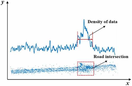
To avoid interference with other traffic, the speed of vehicles will be slowdown and traffic signals are usually assigned in the intersection. As a result, there are significant differences in the distribution of floating car data between road segments and intersections. Compared with the road segment, the data are more dense in the intersection, as shown in Figure 2. Based on this, an Otsu-based background segmentation algorithm is utilized to detect road junctions. First, a Gaussian model is used to resample the data to a grid. To increase the distinction between the segments (background) and intersections (foreground), we utilize a gamma-correction-based spatiotemporal prediction algorithm to process the grid images. Finally, Otsu is introduced to divide the background and foreground features.

Figure 2. Data density difference between road intersections and segments.

3.2.1. Resampling

Resampling is used to transform the GPS data into raster data. A raster can integrate a large amount of GPS data efficiently. A Gaussian model is used to calculate the weight of each grid cell. The cell’s intensity is calculated from the weight of the surrounding GPS points as illustrated in Figure 3(a)

Figure 3. An example of the resampling process.

. P is a grid cell, and B is a buffer with a $3\mathit{\sigma }$ radius ($\mathit{\sigma }$ is relevant to the error of GPS). The weight values of GPS points in B are calculated with Equation (1)(1) $\mathit{W}\left(x_i,y_i\right)=\frac{1}{\sqrt{2\mathit{\pi }}\sigma }exp\left(-\frac{{\left(x_i-x_0\right)}^2+{\left(y_i-y_0\right)}^2}{2{\sigma }^2}\right),\left(x_i,y_i\right)\in \mathit{B}$(1) . The intensity of P is computed by accumulating the weights in buffer B as Equation (2)(2) $\mathit{G}\left(\mathit{P}\right)={\sum }_{\left(x_i,y_i\right)\in \mathit{B}}\mathit{W}\left(x_i,y_i\right)$(2) shows.

(1) $\mathit{W}\left(x_i,y_i\right)=\frac{1}{\sqrt{2\mathit{\pi }}\sigma }exp\left(-\frac{{\left(x_i-x_0\right)}^2+{\left(y_i-y_0\right)}^2}{2{\sigma }^2}\right),\left(x_i,y_i\right)\in \mathit{B}$(1)

(2) $\mathit{G}\left(\mathit{P}\right)={\sum }_{\left(x_i,y_i\right)\in \mathit{B}}\mathit{W}\left(x_i,y_i\right)$(2)

(3) $\mathit{dist}\left(\mathit{P},P_i\right)<3\mathit{\sigma }$(3)

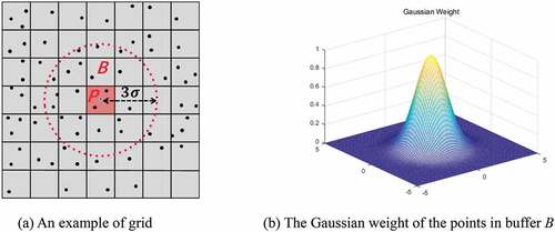
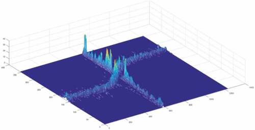
where $\mathit{W}\left(x_i,y_i\right)$ is the weight value of any point $P_i$ in B, $\mathit{G}\left(\mathit{P}\right)$ is the intensity value of grid P, $\mathit{\sigma }$ represents the variance, and $\left(x_0,y_0\right)$ represents the coordinate of the center point of the gird. $(x_i,y_i)$ is the coordinate of GPS point $P_i$. $\mathit{dist}\left(\mathit{P},P_i\right)$ is the distance between $\mathit{P}$ and $P_i$. The result of resampling is depicted in Figure 4. The brighter the color, the greater the intensity value, and the result reveals that the intensity value of intersection points is obviously larger than the GPS points in the road segment.

Figure 4. The result of resampling in a crossroad.

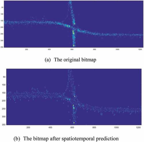
3.2.2. Gamma-correction-based spatiotemporal prediction

As Figure 4 shows, the population of GPS points in intersections is obviously greater than that of points in road segments. With the increase in GPS data, the intensity differences become increasingly distinct. However, the calculation load also increases. To improve the accuracy and efficiency of Otsu, a gamma-correction-based spatiotemporal prediction algorithm is used in this paper. Gamma correction modifies the gamma curve of an image to edit the image non-linearly to detect the dark part and light part in the image, and increase the ratio of the two part to improve the image contrast and is widely used in image processing. We introduce a time coefficient A based on gamma correction as in Equation (4)(4) $I_g=\mathit{A}\ast I_i^{\gamma }$(4) . A is the ratio of target time to test time. The gamma- correction-based spatiotemporal prediction method can increase the variance between the background (segments) and foreground (intersections), which can improve the accuracy of Otsu.

(4) $I_g=\mathit{A}\ast I_i^{\gamma }$(4)

(5) $\mathit{A}=\mathit{T}/T_0$(5)

(6) $I_i=\frac{G_i-G_{\mathit{min}}}{G_{\mathit{max}}-G_{\mathit{min}}},\left\{G_i\in \mathit{G}\mathit{and}{G}_i\ne 0\right\}$(6)

where A is the time coefficient based on the ratio of the prediction time T and to base time $T_0$. $\mathit{\gamma }$ is the separation coefficient between the background and foreground. $I_i$ represents the normalization intensity of the grid. $G_i$ is the density of the gird corresponding to Equation (3)(3) $\mathit{dist}\left(\mathit{P},P_i\right)<3\mathit{\sigma }$(3) . The results of the gamma-correction-based spatiotemporal prediction algorithm are shown in Figure 5. From the figure, it can be seen that the variance between the background and foreground is increased with this method.

Figure 5. An example of a gamma-correction-based spatiotemporal prediction algorithm.

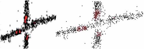
3.2.3. Otsu-based intersections detection

Otsu is a method often used in computer vision and image processing. It assumes that images contain two classes of pixels, background and foreground, and calculates the optimum threshold to maximize the interclass variance and separate the two classes (Otsu 1979). In this paper, we utilize this method to detect intersections from the results of the gamma- correction-based spatiotemporal prediction method. The ratios of intersections and segments are represented by $w_1,w_2$. The mean values are $u_1,u_2$. The interclass variance can be calculated with Equation (7). By traversing different gray thresholds, the relevant ratio and mean value are calculated. Finally, the optimum gray threshold is calculated to classify the road segments and intersections, and the result is illustrated in Figure 6. The red dots indicate the points selected as foreground by Otsu, and the black dots are the background points.

(7) $\mathit{g}=w_1{w}_2{\left(u_1-u_2\right)}^2$(7)

Figure 6. The result of Otsu.

3.3. Clustering

Because the sampling frequency of floating car data ranges from 20s to 60s, the distance between two consecutive GPS points is usually long and changeable. We introduce a clothoid-based method to resample the trajectory. We cluster the trajectories in road segments and road intersections separately, as we have detected the boundary of a road intersection in Section 3.2.

3.3.1. Clothoid-based trajectory resampling

Clothoids are widely used as transition curves in road engineering for their connection to the geometry between tangents and circular curves (Meek and Walton 1992). The curvature of a clothoid changes linearly with its curve length, which is in accordance with the law of vehicle dynamics. Therefore, we utilize a clothoid curve to resample the trajectories. A clothoid curve can be described with an expansion of the Fresnel integral as shown in equations (8)(8) $\mathit{x}\left(\mathit{s}\right)=x_0+{\int }_0^{s}cos\left(\frac{1}{2}\mathit{k}{ }^{\mathrm{\prime }}{\tau }^2+\mathit{k\tau }+{\vartheta }_0\right)\mathit{d\tau },$(8) and (9(9) $\mathit{y}\left(\mathit{s}\right)=y_0+{\int }_0^{s}sin\left(\frac{1}{2}\mathit{k}{ }^{\mathrm{\prime }}{\tau }^2+\mathit{k\tau }+{\vartheta }_0\right)\mathit{d\tau }$(9) ).

(8) $\mathit{x}\left(\mathit{s}\right)=x_0+{\int }_0^{s}cos\left(\frac{1}{2}\mathit{k}{ }^{\mathrm{\prime }}{\tau }^2+\mathit{k\tau }+{\vartheta }_0\right)\mathit{d\tau },$(8)

(9) $\mathit{y}\left(\mathit{s}\right)=y_0+{\int }_0^{s}sin\left(\frac{1}{2}\mathit{k}{ }^{\mathrm{\prime }}{\tau }^2+\mathit{k\tau }+{\vartheta }_0\right)\mathit{d\tau }$(9)

where s is the length of the curve from its start point ($x_{0,}{y}_0$), ${\vartheta }_0$ is the direction of the start point, k is the curvature of the curve at the start point, and k’ is the rate of change of curvature.

In floating vehicle data, the positions of the start and end points and their directions can be deduced. The main problem of generating a clothoid curve between two adjacent GPS points on a trajectory is to calculate the k and k^’ of the clothoid curve. According to the proposed method in reference (Bertolazzi and Frego 2015), the parameters of a clothoid curve can be calculated by the positions and directions of two points as depicted in Figure 7(a)

Figure 7. Clothoid-based trajectory resampling.

. To generate a clothoid curve between two points, the distance d between the points and the incline angle $\mathit{\phi }$ of the line segment are calculated first. Then, the angle between the incline angle $\mathit{\phi }$ and the direction of the start and end points ${\vartheta }_0$, ${\vartheta }_1$ are denoted as ${\mathrm{\varnothing }}_0\mathit{and}{\mathrm{\varnothing }}_1$. The total arc length S_t of the curve is calculated by dividing the value between d and the Fresnel integrals of ${\mathrm{\varnothing }}_0$-${\mathrm{\varnothing }}_1$, ${\vartheta }_0$-${\vartheta }_1$ and ${\mathrm{\varnothing }}_0$. The curvature of the start points $\mathit{k}$ and the rate of curvature change $\mathit{k}{ }^{\mathrm{\prime }}$ is calculated based on the arc length S_t according to reference (Bertolazzi and Frego 2015).

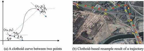
According to the previous step, we create a series of clothoid curves to link the trajectories. To calculate the similarity accurately between different trajectories, we resample the clothoid curve of the trajectories with an arc length step l as shown in Figure 7(b). The orange dots are the original GPS points, and the red points represent the resample points. The blue line is the polyline composed of the original GPS points, and the green line is the clothoid curve composed of the original points and the resample points. The red arrows depict the direction of the original points.

3.3.1. Distance similarity

There is a high probability that two adjacent trajectories belong to the same road. Therefore, we propose a distance-contribution function to calculate the distance similarity of two associated trajectories. As illustrated in Figure 8,

Figure 8. An example of two associated trajectories.

$T_1$ and $T_2$ are two adjacent trajectories $T_1=\left\{p_1,p_2,\cdots ,p_k\right\}$, and $T_2=\left\{q_1,q_2,\cdots ,q_k\right\}$ after resampling by a clothoid curve. We set $T_1$ as the matching trajectory and set $T_2$ as the reference trajectory. In the first step, we calculate the shortest distance $d_i$ from $p_i$ to $T_2$. If $d_i$ < r (r is the distance threshold), then we continue to calculate the discrimination $\mathit{di}{s}_{\mathit{radius}}$ of the turning radius of two points. If $\mathit{di}{s}_{\mathit{radius}}<d_r$ ($d_r$ is the turning radius threshold), as depicted in Figure 9(a),

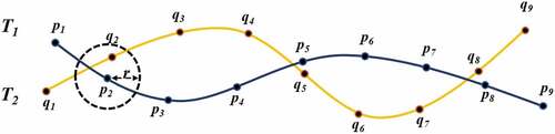
Figure 9. Different scenarios for ${\mathit{f}}_{\mathit{c}\mathit{on}}$.

$\left(d_i<\mathit{rdi}{s}_{\mathit{radius}}<d_r\right)$. We calculate the value of the distance-contribution function $f_{\mathit{con}}$ with Equation (10)(10) $f_{\mathit{con}}=\sqrt{2\mathit{\pi }}\mathit{\sigma }\times exp\left(\frac{r^2}{{\sigma }^2}\right),d_i<\mathit{r}{d}_{\mathit{radius}}<d_r$(10) . If $\mathit{di}{s}_{\mathit{radius}}>d_r$, as shown in Figure 9(b), the value of $f_{\mathit{con}}$ is zero. In addition, if d_i > r at first, as represented in Figure 9(c), the value of $f_{\mathit{con}}$ is zero.

Then, the total value of the distance-contribution function of $T_1$ is calculated with Equation (11)(11) $F_{\mathit{CON}}={\sum }_{\mathit{i}\in \left(1,\mathit{k}\right)}(f_{\mathit{con}}\times \mathit{s})\mathit{\hspace{0.17em}}$(11) . Finally, the distance similarity from $T_1$ to $T_2$ is calculated as the ratio of $F_{\mathit{CON}}$ to the length of $T_2$ as shown in Equation (12)(12) $\mathit{Si}{m}_{\mathit{dis}}=\frac{F_{\mathrm{CON\_}{T}_1}}{\mathit{Le}{n}_{T_2}}$(12) .

(10) $f_{\mathit{con}}=\sqrt{2\mathit{\pi }}\mathit{\sigma }\times exp\left(\frac{r^2}{{\sigma }^2}\right),d_i<\mathit{r}{d}_{\mathit{radius}}<d_r$(10)

(11) $F_{\mathit{CON}}={\sum }_{\mathit{i}\in \left(1,\mathit{k}\right)}(f_{\mathit{con}}\times \mathit{s})\mathit{\hspace{0.17em}}$(11)

(12) $\mathit{Si}{m}_{\mathit{dis}}=\frac{F_{\mathrm{CON\_}{T}_1}}{\mathit{Le}{n}_{T_2}}$(12)

where $d_i$ is the distance from $p_i$ to $T_2$ and $\mathit{\sigma }$ represents the precision of the position. $F_{\mathit{CON}}$ denotes the total value of the distance-contribution function of $T_1$, and $\mathit{Si}{m}_{\mathit{dis}}$ is the distance similarity of $T_1$ and $T_2$. $\mathit{Le}{n}_{T_2}$ represents the length of $T_2$.

3.3.2. Direction similarity

Direction is another important parameter for clustering floating car traces. According to the expansion of a clothoid in Equations (8)(8) $\mathit{x}\left(\mathit{s}\right)=x_0+{\int }_0^{s}cos\left(\frac{1}{2}\mathit{k}{ }^{\mathrm{\prime }}{\tau }^2+\mathit{k\tau }+{\vartheta }_0\right)\mathit{d\tau },$(8) and (9(9) $\mathit{y}\left(\mathit{s}\right)=y_0+{\int }_0^{s}sin\left(\frac{1}{2}\mathit{k}{ }^{\mathrm{\prime }}{\tau }^2+\mathit{k\tau }+{\vartheta }_0\right)\mathit{d\tau }$(9) ), the direction of any point on the curve can be calculated using the arc length to the start point of the curve. Therefore, we can use a piecewise function to calculate the direction of all the resample nodes. When the resampled node is between two GPS points $N_i$ and $N_{\mathit{i}+1}$ of a trajectory, the direction of the resample node can be calculated with Equation (13)(13) $\mathit{D}\left(\mathit{s}\right)={\vartheta }_i+k_i\left(\mathit{s}-s_i\right)+\frac{1}{2}{k}_i^{\mathrm{\prime }}{\left(s-s_i\right)}^2,\mathit{s}\in \left[s_i,s_{\mathit{i}+1}\right],\mathit{i}\in \left(0,\mathit{m}\right)\mathit{\hspace{0.17em}}$(13) .

(13) $\mathit{D}\left(\mathit{s}\right)={\vartheta }_i+k_i\left(\mathit{s}-s_i\right)+\frac{1}{2}{k}_i^{\mathrm{\prime }}{\left(s-s_i\right)}^2,\mathit{s}\in \left[s_i,s_{\mathit{i}+1}\right],\mathit{i}\in \left(0,\mathit{m}\right)\mathit{\hspace{0.17em}}$(13)

where s is the arc length to the start point of the trajectory, ${\vartheta }_i$ is the direction of $N_i$, $k_i$ is the curvature of the curve at $N_i$, and $k_i^{\mathrm{\prime }}$ is the rate of the change in the curvature.

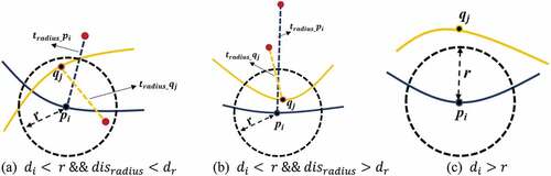
The direction similarity between two trajectories can be calculated using a resample node that meets the distance and turning radius requirements. Figure 9(a) shows a resampling node $q_j$ in the reference trajectory $T_2$ that has a corresponding nearest node $p_i$ in the matching trajectory $T_1$ that meets the distance and turning radius requirements. The direction similarity function can be described, as in Equation (14)(14) $\mathit{Si}{m}_{\mathit{ori}}={\sum }_{i=0}^n\mathit{min}\left(\left|D_1\left(s_i\right)-D_2\left(s_j\right)\right|,\left|D_1\left(s_{p_i}\right)-D_2\left(s_{q_j}\right)\right|-\mathit{\pi }\right)/\mathit{\pi }$(14) .

(14) $\mathit{Si}{m}_{\mathit{ori}}={\sum }_{i=0}^n\mathit{min}\left(\left|D_1\left(s_i\right)-D_2\left(s_j\right)\right|,\left|D_1\left(s_{p_i}\right)-D_2\left(s_{q_j}\right)\right|-\mathit{\pi }\right)/\mathit{\pi }$(14)

3.3.3 Clustering the trajectories

The overall similarity function is calculated by considering both the distance similarity and the direction similarity as in Equation (15)(15) $\mathit{Sim}\left(T_1,T_2\right)=0.5\ast \mathit{Si}{m}_{\mathit{dis}}+0.5\ast \mathit{Si}{m}_{\mathit{ori}}$(15) .

(15) $\mathit{Sim}\left(T_1,T_2\right)=0.5\ast \mathit{Si}{m}_{\mathit{dis}}+0.5\ast \mathit{Si}{m}_{\mathit{ori}}$(15)

A hierarchical clustering method is used to classify all the trajectories in the intersections for different turning directions.

Step 1: All the trajectories are marked as “unused”, and the base clusters are initialized to empty.

Step 2: Two trajectories are chosen and their similarity value is calculated. If the similarity is less than a given threshold $T_g$, two different clusters are added to the base clusters, and the trajectories are marked as the corresponding base cluster index.

Step 3: The following trajectories are compared to all the list clusters. If the similarity between one trajectory of the list is larger than the given threshold, the trajectory is added to that cluster. If the similarity value to all the list clusters is smaller than the given threshold, the trajectory is realized as a new cluster and added to the base clusters.

Step 4: After all the trajectories of the intersection are clustered, the clusters that have more than N trajectories are selected.

3.4. Centerline extraction

In the clustering result for an intersection, the trajectories having the same direction contain many discrete points that have certain aggregation characteristics. A piecewise weighted least square fitting method is used to extract the centerline of the clusters. The detailed step of the proposed method are as follows:

Step 1: A rectangular fitting region is created in front of the entry point of the cluster. The direction of the region is the same as the direction of the entry point as shown in Figure 10.

Figure 10. An example of a rectangular fitting region.

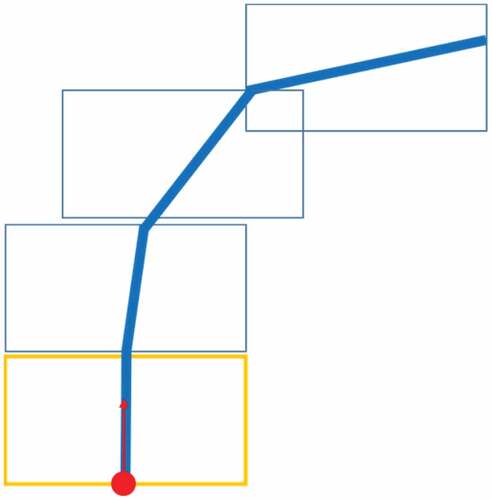
Step 2: Corresponding bitmap generated in Section 3.2 that corresponds to the rectangular region are selected if they contain intensities greater than the threshold $T_i$ The selected girds are designed as the key points to fit the line segments of the region.

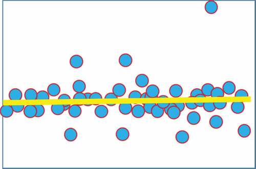
Step 3: A weighted least squares fit is used to compute the parameters of the line segment of the region. The weights of the key points are the normalized values of their intensities. The result of the weighted least squares fitting is shown in Figure 11.

Figure 11. An example of weighted least squares fitting.

The fitting line segment of the rectangular region can be described as follows:

(16) $\mathit{f}\left(\mathit{x}\right)=\mathit{ax}+\mathit{b}$(16)

The residual error E of fitting the line segment under weight W is shown as Equation (17)(17) $\mathit{E}={\sum }_{i=0}^n{W}_i\times \left(\mathit{f}\left(x_i\right)-y_i\right)$(17) .

(17) $\mathit{E}={\sum }_{i=0}^n{W}_i\times \left(\mathit{f}\left(x_i\right)-y_i\right)$(17)

By minimizing the residual error E, the parameter matrix $\mathit{c}={\left[\mathit{a},\mathit{b}\right]}^{\mathrm{T}}$ can be calculated with Equation (18)(18) $\mathit{c}={\left({\mathit{A}}^{\mathrm{T}}\mathit{WA}\right)}^{-1}{A}^{\mathrm{T}}\mathit{Wb}$(18) .

(18) $\mathit{c}={\left({\mathit{A}}^{\mathrm{T}}\mathit{WA}\right)}^{-1}{A}^{\mathrm{T}}\mathit{Wb}$(18)

where A and b are the matrix styles of the horizontal and vertical coordinates, respectively, and W is the weight matrix.

(19) $\mathit{A}=\left[\begin{array}{cc}1& x_1\\ ⋮& ⋮\\ 1& x_n\end{array}\right],\mathit{\hspace{0.17em}}\mathit{b}=\left[y_1\cdots y_n\right],\mathit{W}=\left[\begin{array}{c}{W}_1\\ \ddots \\ W_n\end{array}\right]\mathit{\hspace{0.17em}}$(19)

Step 4: Sequences of line segments are extracted along with the cluster in Step 1 to Step 3. The direction of the next rectangular region is replaced with the direction of the current rectangular region.

Step 5: A clothoid curve is used to fit the global segments of the clusters, which can make the centerline smooth and more like the real road.

3.5. Road network building

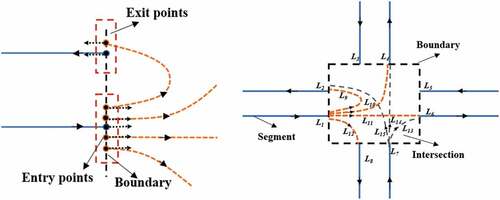
Because we calculate the boundary of an intersection in section 3.2.3, the traces are divided into two parts: road segment and intersection. The cutting points are the crossing points of the centerline of the clustered data and the boundary of the intersection. If the direction of a point is toward the inside of a road intersection, it is defined as an entry point. Otherwise, it is defined as an exit point as depicted in Figure 12. If the start point of a road can be matched with the endpoint of another road, it means that the two roads are connected. As shown in Figure 12, $L_1$ is connected to $L_9$ $L_{10}$, $L_{11}$ and $L_{12}$. The road segments are connected by road intersections. The connectivity attribute of Figure 12 is expressed in Table 1.

Figure 12. An example of building a road network.

Table

Exit Entry	L2	L4	L6	L8
L1	L9	L10	L11	L12
L7	L15	L14	L13	0

4. Experimental results and discussions

To evaluate the proposed approach, experiments are conducted on two datasets in Wuhan, China. In this section, we first introduce two datasets and the parameters used in this paper. Thereafter, we show the results of intersection detection, clustering and centerline extraction. Then, we compare and evaluate the proposed method with the two other methods. Finally, we discuss the advantages and disadvantages of the proposed method.

4.1. Experimental data and parameters

To test the method proposed in this paper, we use two datasets collected by thousands of vehicles in Wuhan, China. Figure 13(a) illustrates data 1, which contains 700,000 track points and was cleaned in our previous study (Li et al. 2018). The sampling frequency of the data ranges from 20 s to 60 s and the position accuracy ranges from 5 m to 30 m. Figure 13(b) illustrates the original floating car data (data 2). We collected approximately 1.4 million track points in one week. The parameter setting values are shown in Table 2.

Figure 13. The experimental floating car data.

Table 2. The parameter setting values

Intersection detection			clustering
$\mathit{\sigma }$	$\mathit{A}$	r	l	$\mathit{r}$	$d_r$	Tg	N	Ti
30	12	2	5	10	20	0.45	10	6

In this article, some parameters need to be set. First, $\mathit{\sigma }$ is relevant to the GPS error, and we set $\mathit{\sigma }=30$. A means the time coefficient in the gamma-correction-based spatiotemporal prediction process. In our study, $\mathit{A}=12$. $\mathit{\gamma }$ is the separation coefficient between the background and foreground. The arc length step $\mathit{l}$ is used to resample the clothoid curve of the trajectories, and we set $\mathit{l}=5$ for this paper. Between two different trajectories, the distance threshold r and turning radius threshold $d_r$ are used to calculate their distance similarity. We set r = 10 m and $d_r$ = 20 m. To cluster all the trajectories, we use a threshold $T_g$ to decide whether different trajectories are similar to each other. When the number of a cluster is more than N, the cluster is selected as a director of the intersection. We set $T_g$ = 0.45 and N = 10.

For centerline extraction, the centerlines of the clusters are generated along the trajectories by a series of rectangular regions. The bitmaps of the rectangular regions are used in this step. The intensities of the grid cells that are larger than $T_i$ are selected as key points to fit the centerline segment in this rectangular region with the least squares method. In addition, we set $T_i$ = 6 for this paper.

4.2. Results

4.2.1. Intersection detection results

The results of intersection detection in data 1 are depicted in Figure 14. Figure 14(a)

Figure 14. The results of intersection detection in data 1.

shows the results of Otsu, and the detection results are shown in Figure 14(b). Each circle presents the spatial coverage of the intersection. There are four kinds of results by manual inspection: correctly detected, incorrectly detected, correctly excluded and not detected.

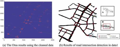
As the area of data 1 is one of the CBDs of Wuhan, there is high traffic flow and often traffic jams there. However, more than 92% of the intersections are correctly detected by our method, indicating the validity of the Otsu-based intersection detection algorithm. There is one road intersection not detected, as shown in rectangle A. The main reason for not being detected in A is that the variation of the data density in this intersection is not obvious compared with the nearby road segments. In addition, three intersections are incorrectly detected. As shown in rectangle B, the density of data in the red rectangle is greater than that of the near data as it is the entrance to a community, as a result, these data are incorrectly detected as intersections.

The results of intersection detection in data 2 are depicted in Figure 15.

Figure 15. The results of intersection detection in data 2.

Data 2 is the original floating car data that are full of noise points. Compared with data 1, data 2 contains more road scenarios and is more complex. However, from Figure 15(a,b), we can see that more than 85% of the road intersections are accurately detected by our method, demonstrating the robustness of the algorithm.

Some of the minor intersections are not detected or are incorrectly detected. For instance, intersections C and D in Figure 15(b) are not detected. The main reason is that there are few vehicles turning at these intersections, so the data density is not significantly different than the surrounding data. In this case, Otsu cannot tell the foreground from the background. Additionally, intersections E and F are incorrectly detected, and the main reasons for the “incorrectly detected” are that on these roads, there is frequent traffic blockage or there is a community or shopping mall entrance and many vehicles stop there. Therefore, the data density is significantly greater than that of the surroundings.

4.2.2. Results of clustering and centerline extraction

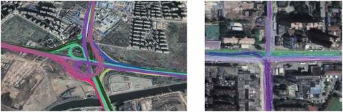
In the data clustering part, we use a clothoid-based method to resample the GPS trajectory first. The clothoid-curve can correctly resample the trajectory to make it closer to the real trajectory of the vehicle, and the accuracy of clustering is not affected by the low sampling frequency of floating cars after clothoid-based resampling. Then, we calculate the distance and direction similarity of the trajectories to cluster them. Data with greater distance and direction similarity have a greater probability of belonging to the same cluster. We use satellite images as the background for comparison with the clustering and centerline extraction results as shown in Figure 16. The results demonstrate that the proposed clustering and centerline extraction method can correctly delineate the geometries of road intersections and segments.

Figure 16. The results of clustering in different road intersections.

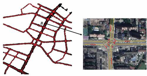
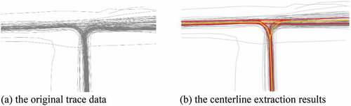
The result of centerline extraction is illustrated in Figure 17. Most road segments and intersections are correctly extracted. In addition, the clothoid curve is also used in the centerline extraction part to fit the global segments of the clusters, which can make the centerline smoother and closer to the real road compared with a polyline. The position accuracy of the road network can reach 2 m to 5 m.

Figure 17. Centerline extraction results of data 1.

4.2.3. Results comparison and evaluation

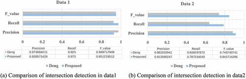
In the intersection detection step, we compare the proposed method with the algorithm proposed by Deng et al. (2018) through three indicators precision, recall, and F value in data 1 and data 2, illustrated in Equation (20–22). Deng detected intersections by a hotspot analysis, and we detected intersections through a computer-vision based OTSU method. The comparative results of the two methods are shown in Figure 18. The recall value of our method is higher than Deng’s method for data 1. However, the precision of our method is lower than that of the method by Deng. The main reason for the result is that our method is sensitive to the data density change. The roads where a traffic block frequently form are easily recognized as intersections by our algorithm. For data 2, road scenarios are complex and data quality is low. However, our method achieved higher precision value and significantly higher recall value and F value than Deng’s method, which proved the robustness of our method for intersection detection.

(20) $\mathrm{precision}=\frac{\mathrm{correctly}\mathrm{detected}}{\mathrm{correctly}\mathrm{detected}+\mathrm{incorrectly}\mathrm{detected}}$(20)

(21) $\mathrm{recall}=\frac{\mathrm{correctly}\mathrm{detected}}{\mathrm{correctly}\mathrm{detected}+\mathrm{not}\mathrm{detected}}$(21)

(22) $\mathrm{F}-\mathrm{value}=\frac{2\ast \mathrm{precision}\ast \mathrm{recall}}{\mathrm{presion}+\mathrm{recall}}$(22)

Figure 18. Results comparison of intersection detection.

In addition, in the centerline extraction parts, we compare our method with the existing algorithm proposed by Biagioni and Eriksson (2012). The author proposed a classic map inference method. First, the author extracted the map centerline from density estimate data through a grayscale map skeletonization method. Then, the author pruned and merged the edge and intersection based on a trajectory-based topology refinement technique. Finally, the author estimated intersection geometries by a trajectory-based geometric refinement technique. We used a manually interpreted section of OpenStreetMap as ground truth. The method proposed in reference (Liu et al. 2012b) is used to perform a quantitative measurement of the two methods. In reference (Liu et al. 2012b), the author performed a quantitative evaluation by measuring the precision and recall of the inferred map M and ground truth map $T_m$. In addition, the author determined the true positive length $T_p=\mathit{M}{\cap }^{T_m}$ as a measure of common road length. To calculate the true positive length $T_p$, we sample the map at 5 m intervals first and then compute it by one-to-one map matching.

(23) $\mathrm{precision}=\frac{T_p}{∥\mathit{M}∥}$(23)

(24) $\mathrm{recall}=\frac{T_p}{∥T_m∥}$(24)

The comparison result is shown in Figure 19. In data1 and data 2, the proposed method achieved a significantly higher precision and recall value. The main reason is that the proposed method clustered the data first and extracted the centerline of the road from the clustering results, which can describe the geometry of the road more specifically. In addition, we use a clothoid-based trajectory resampling algorithm to increase the density of data, which also improves the accuracy of the results, as shown in Figure 20.

Figure 19. Results comparison of centerline extraction.

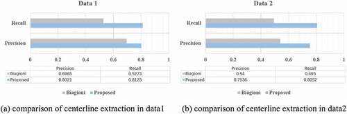
Figure 20. Results comparison of centerline extraction. Red lines represent the results of our method, and the yellow lines are the results of Biagioni.

4.3. Discussion

The overall method of this paper can be divided into two parts: (1) intersection detection and (2) data clustering and centerline extraction. In the first part, we experimented with the algorithm on two datasets and compared our method with Deng’s. The results show that our method can achieve an obviously higher recall value, which proves the robustness of our method. However, the precision of the algorithm needs to be further improved, as it is sensitive to data density changes. The roads where a traffic block frequently formed or the entrance to a shopping mall may be recognized as intersections. But in general, the method in this paper can achieve better results in complex environments as we use a computer-vision based OTSU method. In our future work, we will consider the direction change of the data at the intersection, combine the direction change and density difference of road intersections and segments, and try to use machine learning to extract road intersections. In part two, we compared our method with Biagioni’s. The algorithm in this article achieved a higher precision and recall value. Our method can describe the geometry and topology of roads in more detail, because we resample the trajectories based on clothoid curves and cluster the data in different classes. However, in places where GPS satellite coverage is severely occluded, trajectory errors will make it impossible to resample, which will affect the results of clustering and centerline extraction. In our future work, we will try to incorporate the image data to infer higher precision road information.

5. Conclusions

In this paper, we proposed a novel method to mine road networks from floating car data. We first presented an Otsu-base algorithm in the intersection detection part, which is the first time using this method in intersection detection. In the clustering step, we proposed a clothoid-based method to resample the trajectory for improved cluster accuracy. Then, a distance-direction method was used to cluster the data. Last, a piecewise weighted least square fitting method was used to extract the cluster centerlines. We compared the proposed method with others. Our method can detect intersections effectively and robustly, and the extracted road centerline is more accurate and smoother than other algorithms. The geometric information and topological structure of the road are important parts of HD maps. Our method can be used to update the road map and provide a geometric basis for the HD map, and in our future work, we can try to extract more detailed and accurate road information and build a complete HD map.

Disclosure statement

No potential conflict of interest was reported by the author(s).

Data availability statement

The data that support the findings of this study are available from DF GO. DF GO is a mobility technology platform. It offers app-based services including taxi-hailing. Restrictions apply to the availability of these data, which were used under license for this study. Data are available with the permission of DF GO (www.dfcx.com.cn).

Additional information

Funding

This work is supported by the Joint Fund for Innovation and Development of Automobile Industry of National Natural Science Foundation of China [Grant Number U1764262], the National Natural Science Foundation of China [Grant Number 42101448].

Notes on contributors

Yuan Guo

Yuan Guo .

Bijun Li

Bijun Li is a professor in the State Key Laboratory of Information Engineering in Surveying, Mapping and Remote Sensing (LIESMARS), Wuhan University. He received the PhD degree from Wuhan University in 2008. His research interests are mostly focused on navigation and location services, intelligent driving, and vehicle-road collaboration.

Zhi Lu

Zhi Lu is a PhD student in the State Key Laboratory of Information Engineering in Surveying, Mapping and Remote Sensing (LIESMARS), Wuhan University. His research interests include autonomous driving and intelligent transportation system.

Jian Zhou

Jian Zhou received the PhD degree in cartography and geographic Information system from the Wuhan University in 2019. He is currently a postdoc with The State Key Laboratory of Information Engineering in Surveying, Mapping and Remote Sensing (LIESMARS) of Wuhan University. His research interests include high-accuracy map, computer vision, and autonomous vehicles.

References

- “Roadmap” 2021. “Wikipedia.” https://en.wikipedia.org/w/index.php?title=Roadmap.
- Ahmed, M., S. Karagiorgou, D. Pfoser, and C. Wenk. 2015. “A Comparison and Evaluation of Map Construction Algorithms Using Vehicle Tracking Data.” GeoInformatica 19 (3): 601–632. doi:10.1007/s10707-014-0222-6.
- Bertolazzi, E., and M. Frego. 2015. “G1 Fitting with Clothoids.” Mathematical Methods in the Applied Sciences 38 (5): 3. doi:10.1002/mma.3114.
- Biagioni, J., and J. Eriksson. 2012. “Map Inference in the Face of Noise and Disparity.” In International Conference on Advances in Geographic Information Systems, 79–88. New York, NY.
- Bruntrup, R., S. Edelkamp, S. Jabbar, and B. Scholz. 2005. “Incremental Map Generation with GPS Traces.” In Intelligent Transportation Systems, 2005. Proceedings, 574–579. Vienna, Austria.
- Cao, L., and J. Krumm. 2009. “From GPS Traces to a Routable Road Map.” In The Workshop on Advances in Geographic Information Systems, 3–12. New York, NY.
- Chen, B., C. Ding, W. Ren, and G. Xu. 2020. “Extended Classification Course Improves Road Intersection Detection from Low-Frequency GPS Trajectory Data.” Isprs International Journal of Geo-Information 9 (3): 181. doi:10.3390/ijgi9030181.
- Chen, C., and Y. Cheng. 2008. “Roads Digital Map Generation with Multi-Track GPS Data.” In International Workshop on Education Technology and Training & 2008 International Workshop on Geoscience and Remote Sensing , 508–511. Shanghai China.
- Chen, Y., and J. Krumm. 2010. “Probabilistic Modeling of Traffic Lanes from GPS Traces.” In Sigspatial International Conference on Advances in Geographic Information Systems, 81–88. New York, NY.
- Deng, M., J. Huang, Y. Zhang, H. Liu, L. Tang, J. Tang, and X. Yang. 2018. “Generating Urban Road Intersection Models from Low-Frequency GPS Trajectory Data.” International Journal of Geographical Information Science 32 (12): 2337–2361. doi:10.1080/13658816.2018.1510124.
- Fang, W., H. Rong, X. Xiang, Y. Xia, and M.H. Hung. 2016. “A Novel Road Network Change Detection Algorithm Based on Floating Car Tracking Data.” Telecommunication Systems, March.
- Fathi, A., and J. Krumm. 2010. “Detecting Road Intersections from GPS Traces.” In Geographic Information Science, edited by Fabrikant, S.I., Reichenbacher, T., van Kreveld, M., and Schlieder, C. Lecture Notes in Computer Science, 56–69. Berlin, Heidelberg: Springer.
- Guo, T., K. Iwamura, and M. Koga. 2007. “Towards High Accuracy Road Maps Generation from Massive GPS Traces Data.” In 2007 IEEE International Geoscience and Remote Sensing Symposium, 667–670. Barcelona, Spain.
- Gwon, G.P., W.S. Hur, S.W. Kim, and S.W. Seo. 2017. “Generation of a Precise and Efficient Lane-Level Road Map for Intelligent Vehicle Systems.” IEEE Transactions on Vehicular Technology 66 (6): 4517–4533. doi:10.1109/TVT.2016.2535210.
- Huang, B., and J. Wang. 2020. “Big Spatial Data for Urban and Environmental Sustainability.” Geo-Spatial Information Science 23 (2): 125–140. doi:10.1080/10095020.2020.1754138.
- Jo, K., and M. Sunwoo. 2014. “Generation of a Precise Roadway Map for Autonomous Cars.” IEEE Transactions on Intelligent Transportation Systems 15 (3): 925–937. doi:10.1109/TITS.2013.2291395.
- Karaduman, M., A. Cinar, and H. Eren. 2019. “UAV Traffic Patrolling via Road Detection and Tracking in Anonymous Aerial Video Frames.” Journal of Intelligent & Robotic Systems 95 (2): 675–690. doi:10.1007/s10846-018-0954-x.
- Li, B., Y. Guo, J. Zhou, and Y. Cai. 2018. “A Data Correction Algorithm for Low-Frequency Floating Car Data.” Sensors 18 (11): 3639–3656.
- Li, J., Q. Qin, C. Xie, and Y. Zhao. 2012. “Integrated Use of Spatial and Semantic Relationships for Extracting Road Networks from Floating Car Data.” International Journal of Applied Earth Observations & Geoinformation 19 (1): 238–247. doi:10.1016/j.jag.2012.05.013.
- Liu, X., J. Biagioni, J. Eriksson, Y. Wang, G. Forman, and Y. Zhu. 2012a. “Mining Large-Scale, Sparse GPS Traces for Map Inference: Comparison of Approaches.” In Proceedings of the 18th ACM SIGKDD International Conference on Knowledge Discovery and Data Mining. KDD ’12, 669–677. New York, NY: Association for Computing Machinery.
- Liu, X., Y. Zhu, Y. Wang, G. Forman, L.M. Ni, Y. Fang, and M. Li. 2012b.” Road recognition using coarse-grained vehicular traces.“ Tech. rep. HPL-2012-26 . HP Laboratories.
- Massow, K., B. Kwella, N. Pfeifer, F. Haeusler, J. Pontow, I. Radusch, J. Hipp, F. Doelitzscher, and M. Haueis. 2016. “Deriving HD Maps for Highly Automated Driving from Vehicular Probe Data.” 2016 IEEE 19th International Conference on Intelligent Transportation Systems (ITSC). New York: IEEE.
- Meek, D. S., and D. J. Walton. 1992. “Clothoid Spline Transition Spirals.” Mathematics of Computation 59 (199): 117–133. doi:10.1090/S0025-5718-1992-1134736-8.
- Otsu, N. 1979. “A Threshold Selection Method from Gray-Level Histograms.” IEEE Transactions on Systems, Man, and Cybernetics 9 (1): 62–66. doi:10.1109/TSMC.1979.4310076.
- Sester, M. 2020. “Analysis of Mobility Data – A Focus on Mobile Mapping Systems.” Geo-Spatial Information Science 23 (1): 68–74. doi:10.1080/10095020.2020.1730713.
- Shi, W., S. Shen, and Y. Liu. 2009. “Automatic Generation of Road Network Map from Massive GPS, Vehicle Trajectories.” In International IEEE Conference on Intelligent Transportation Systems, 1–6. St. Louis, Mo.
- Tang, L., X. Yang, Z. Dong, and Q. Li. 2016. “CLRIC: Collecting Lane-Based Road Information Via Crowdsourcing.” IEEE Transactions on Intelligent Transportation Systems 17 (9): 2552–2562. doi:10.1109/TITS.2016.2521482.
- Wang, H., Y.Y. Hou, and M. Ren. 2017. “A Shape-Aware Road Detection Method for Aerial Images.” International Journal of Pattern Recognition and Artificial Intelligence 31 (4): 1750009. doi:10.1142/S0218001417500094.
- Wang, J., X. Rui, X. Song, X. Tan, C. Wang, and V. Raghavan. 2015. “A Novel Approach for Generating Routable Road Maps from Vehicle GPS Traces.” International Journal of Geographical Information Systems 29 (1): 69–91. doi:10.1080/13658816.2014.944527.
- Winden, K.V., F. Biljecki, and S. Van Der Spek. 2016. “Automatic Update of Road Attributes by Mining GPS Tracks.” Transactions in Gis 20 (5): 664–683. doi:10.1111/tgis.12186.
- Wu, H., Z. Gui, and Z. Yang. 2020. “Geospatial Big Data for Urban Planning and Urban Management.” Geo-Spatial Information Science 23 (4): 273–274. doi:10.1080/10095020.2020.1854981.
- Yang, X., L. Tang, L. Niu, X. Zhang, and Q. Li. 2018. “Generating Lane-Based Intersection Maps from Crowdsourcing Big Trace Data.” Transportation Research Part C Emerging Technologies 89: 168–187. doi:10.1016/j.trc.2018.02.007.
- Yuan, J., and A.M. Cheriyadat. 2016. “Image Feature Based GPS Trace Filtering for Road Network Generation and Road Segmentation.” Machine Vision and Applications 27 (1): 1–12. doi:10.1007/s00138-015-0722-x.
- Zhang, X., X. Han, L. Chen, X. Tang, H. Zhou, and L. Jiao. 2019. “Aerial Image Road Extraction Based on an Improved Generative Adversarial Network.” Remote Sensing 11 (8): 930. doi:10.3390/rs11080930.
- Zheng, K., and D. Zhu. 2019. “A Novel Clustering Algorithm of Extracting Road Network from Low-Frequency Floating Car Data.” Cluster Computing 22 (S5): 12659–12668. doi:10.1007/s10586-018-1718-x.
- Zuo, Y., Z. Liu, and X. Fu. 2020. “Measuring Accessibility of Bus System Based on Multi-Source Traffic Data.” Geo-Spatial Information Science 23 (3): 248–257. doi:10.1080/10095020.2020.1783189.