Population spatialization with pixel-level attribute grading by considering scale mismatch issue in regression modeling

ABSTRACT

Population spatialization is widely used for spatially downscaling census population data to finer-scale. The core idea of modern population spatialization is to establish the association between ancillary data and population at the administrative-unit-level (AU-level) and transfer it to generate the gridded population. However, the statistical characteristic of attributes at the pixel-level differs from that at the AU-level, thus leading to prediction bias via the cross-scale modeling (i.e. scale mismatch problem). In addition, integrating multi-source data simply as covariates may underutilize spatial semantics, and lead to incorrect population disaggregation; while neglecting the spatial autocorrelation of population generates excessively heterogeneous population distribution that contradicts to real-world situation. To address the scale mismatch in downscaling, this paper proposes a Cross-Scale Feature Construction (CSFC) method. More specifically, by grading pixel-level attributes, we construct the feature vector of pixel grade proportions to narrow the scale differences in feature representation between AU-level and pixel-level. Meanwhile, fine-grained building patch and mobile positioning data are utilized to adjust the population weighting layer generated from POI-density-based regression modeling. Spatial filtering is furtherly adopted to model the spatial autocorrelation effect of population and reduce the heterogeneity in population caused by pixel-level attribute discretization. Through the comparison with traditional feature construction method and the ablation experiments, the results demonstrate significant accuracy improvements in population spatialization and verify the effectiveness of weight correction steps. Furthermore, accuracy comparisons with WorldPop and GPW datasets quantitatively illustrate the advantages of the proposed method in fine-scale population spatialization.

KEYWORDS:

• Random forest (RF)
• point of interests (POIs)
• mobile positioning data
• natural breaks
• spatial filtering
• population mapping
• dasymetric downscaling

1. Introduction

The population distribution data with fine spatial resolution is critical for urban planning (Bakillah et al. 2014; Dong et al. 2017), disaster prevention (Ahola et al. 2007; Aubrecht et al. 2016), public health (Fecht et al. 2020), and socioeconomic activities analyses (Li et al. 2018a). Census data typically reported at AU-level is authoritative, normative but in coarse resolution; thus, it is hard to reveal the spatial heterogeneity of population distribution within statistical district and in turn benefit various applications. Generally, detailed population distribution can be acquired by redistributing coarse administrative unit level population data to a finer scale (e.g. pixel-level) through downscaling approach (Sinha et al. 2019; Ye et al. 2019). During the past decades, some methods have been proposed to produce fine-scale population gridded data sets at global and region level for supporting various applications (Leyk et al. 2019). For example, area weighting (Lwin 2010; Goodchild and Lam 1980) was used to produce Gridded Population of the World (GPWv4, 1 km resolution), while dasymetric mapping (Zhao et al. 2019; Ye et al. 2019; Stevens et al. 2015) was applied to generate LandScan (1 km resolution) and WorldPop (100 m resolution). Among these methods, dasymetric mapping has been demonstrated to be more effective in generating more accurate population estimates than other approaches (Mennis and Hultgren 2006; Stevens et al. 2015; Zhao et al. 2019).

Although dasymetric mapping methods are widely used techniques (Nagle et al. 2014), the issues associated with cross-scale modeling is often overlooked (Sinha et al. 2019). Meanwhile, the underutilization of semantic information and the neglect of autocorrelation of population also limit the accuracy of population spatialization. The main idea of dasymetric mapping is to generate a gridded prediction of population density, which is then used as the weighting layer to perform dasymetric redistribution of the census counts (Zhao et al. 2019). Due to the lack of actual population at fine-scale, the association between the modeling factors and population is constructed at AU-level, then transferred to predict the gridded population. However, there is a mismatch that exists between training and prediction data under a change of scale, resulting in low accuracy of population estimation (Bai, Wang, and Yang 2013; Sinha et al. 2019; Dong, Yang, and Cai 2016b). Additionally, the accuracy of population spatialization significantly depends on the features used. Semantic information embodied in multi-source data can be used jointly to support more accurate population spatialization. For instance, the spatial distribution of resident population is constrained by building in physical world; hence, building data can be used to alleviate the overestimation of population from POI-density-based modeling in suburban areas (Wang, Fan, and Wang 2020). Mobile positioning data record human activities in a particular time and locations, which can be utilized to balance the population estimation deviation (Yang et al. 2019). Whereas in the context of dasymetric mapping, semantic information is likely underutilized in existing studies, where multi-source data are mostly integrated as covariates for model training (Ye et al. 2019; Stevens et al. 2015). What’s more, the neglect of the characteristic of spatial autocorrelation in geography phenomena lead to the overdiscretization of the generated population data that may contradict to the real population distribution, especially when fine-grained and discrete data are used in modeling (Du, Zhang, and Zhang 2007).

To tackle the abovementioned issues, this paper proposed a cross-scale population spatialization method, and explored its effectiveness in different districts and streets with different population densities. The main contributions are listed as follows:

• Rather than simply counting attribute statistics at each pixel, CSFC grades pixels according to pixel-level attributes (e.g. counts of POIs) and then calculates the proportion of pixel grades at AU-level, which can reduce the scale differences in feature representation between training and prediction, hence ameliorate the scale mismatch problem of statistical unit in cross-scale modeling.

• To adjust population weights for better disaggregation, we fuse building patch and mobile positioning data that refine the spatial coverage of population and balance the estimation bias generated from urban facility POI-based modeling.

• Gaussian spatial filtering is incorporated to model the autocorrelation of population and avoid overdiscretization problem of population distribution. Besides, we analyzed its validity by exploring the influence of pixel resolution, size of filtering template on the accuracy of population spatialization at different districts.

The remainder of the paper is organized as follows. Related work is provided in the next section. The approach is demonstrated in Section 3. Section 4 presents the experiments and the discussion of results. Section 5 concludes the paper and outlines future work.

2. Related work

2.1. Modeling methods of population spatialization

Representative methods for population spatialization can be categorized into spatial interpolation, statistical modeling and deep learning methods.

Spatial interpolation is implemented based on Tobler’s First Law of Geography, which believes near things are more related than distant things (Tobler 1970), but it is usually hard to achieve fine-scale population spatialization (Bai, Wang, and Yang 2013; Wu, Qiu, and Wang 2005). Area weighting assumes the population to be uniformly distributed and transforms it according to the overlapping area (Lwin 2010; Goodchild and Lam 1980). The distance-decay models interpolate according to the decreasing trend of urban population density from the center to the outside, such as negative index model (Clark 1951), Gaussian model (Smeed 1963), and gravity-based model (Wang and Guldmann 1996). Inconsistent with the classical urban geography theories, the urban polycentricity of modern cities and the irregular urban area lead to uncertainties and errors in estimation (Bai, Wang, and Yang 2013). The results obtained by simple interpolation are of coarse resolution and low precision (Fan et al. 2004), while sophisticated interpolation models need to combine varieties of auxiliary data and is also difficult to transfer from region to region due to that different regions may follow different laws.

Statistical modeling methods aim to establish the regression model between multi-source data and population (Nagle et al. 2014; Wu, Qiu, and Wang 2005) and are widely adopted in recent studies. Multivariate Linear Regression model is usually applied to large-scale population estimation but of insufficient fineness (Zeng et al. 2011; Zhuo et al. 2005). Spatial regression models make use of the geographic location and spatial accumulation characteristics of the study data, but specifying the appropriate spatial weight matrix and bandwidth remains a challenge (Brunsdon, Fotheringham, and Charlton 1998; Lo 2008; De Knegt et al. 2010; Chen 2018). By contrast, random forest (RF), a machine learning model evolved from decision trees, can cope with high-dimensional features and improve the spatial precision of population spatialization (Ye et al. 2019; Stevens et al. 2015; Sinha et al. 2019; Breiman 2001, 1996). As a result, the focus can be placed on how to effectively integrate multi-source data and construct features in regression, which may affect the accuracy significantly. However, existing studies simply model with attributes in each pixel and ignore neighboring influence and spatial autocorrelation of population. What’s more, aforementioned regression methods generally establish association between modeling factors and the population at the administrative-unit and then transfer it to pixel-level for achieving population estimation. However, modeling finer scale distribution with coarser scale training data will incur the underestimation of extreme values (Sinha et al. 2019).

In the past few years, deep learning has been applied in population spatialization (Tiecke et al. 2017; Doupe et al. 2016; Robinson, Hohman, and Dilkina 2017; Zhao et al. 2020). Satellite image pixels can be converted into gridded population estimates by training Convolutional Neural Networks (CNNs) (Doupe et al. 2016; Robinson, Hohman, and Dilkina 2017). Unfortunately, the lack of pixel-level training data makes such conversion impractical in real-world applications. By detecting large-scale building footprints from satellite imagery with computer vision technology, Facebook Connectivity Lab allocates the statistical population to the buildings equally (Tiecke et al. 2017). However, how to accurately distribute population counts to building structures need to be further studied. In country-level population spatialization, CNNs and Deep Neural Networks (DNNs) learn representations from multisource data better than shallow machine learning (e.g. RF) and achieve a higher quality (Zhao et al. 2020). Nevertheless, the insufficient training samples make it hard to model with deep learning methods at city-level population spatialization.

In summary, regression modeling is a practical and prevailing solution for generating large-scale and fine-grained population dataset, while RF provides a promising approach for yielding reliable spatialization results. It can model complex nonlinear associations between predictions and heterogeneous predictor variables and achieve high accuracy and stability. Besides the modeling methods, spatialization accuracy is also affected by the selection of ancillary data; hence, more attention should be paid on how to effectively integrating multi-source data.

2.2. Integration of multi-source data in population spatialization

With the development of remote sensing, volunteer geographic information and global positioning technologies, the acquisition of multi-source geospatial data has been greatly facilitated. The ancillary data of population spatialization is becoming more multi-sourced, fine-grained, and dynamic (Dong, Yang, and Cai 2016b; Wu, Gui, and Yang 2020).

The spatial distribution of population is affected by many factors, such as geographic location, land cover, convenience of road networks, water areas, and economic development (Wu and Gao 2010; Xiao et al. 2010). As important indicators for reflecting human activities, land cover and nighttime light (NTL) imagery have been widely adopted for disaggregating census population (Sutton et al. 2001; Jia and Gaughan 2016; Zeng et al. 2011). Land use data can describe the overall spatial coverage of population but is difficult to reveal the heterogeneity of population density under the same land type, while the intensity of NTL data compensates for this shortcoming but with the problem of excessive high light radiance (Yu et al. 2019; Zheng et al. 2020). A recent trend is integrating diverse data sources (Stevens et al. 2015; Bai et al. 2015) to enrich the representation of population distribution, such as water body, networks of roads, DEM, etc. More data provide more comprehensive auxiliary information and spatial constraints for better population disaggregation. However, these ancillary data are coarse-grained and inadequate to reflect refined spatial distribution of population.

Fine-grained modeling data has more detailed location and spatial semantics, which are capable to support fine-resolution population mapping. As a type of social sensing data, different types of facility POIs have different levels of attraction to population (Bakillah et al. 2014). POIs have been combined with NTL imagery data for population spatialization (Yang et al. 2019; Ye et al. 2019; Wang, Fan, and Wang 2020); these approaches mainly build POI-density-based indexes for regression modeling. Moreover, POIs have been utilized to define urban functional districts to assist population disaggregation (Gao, Janowicz, and Couclelis 2017; Li, Chen, and Li 2018). Although POIs reflect potential social activities surrounding or within them, they cannot accurately describe the distribution range of resident population. Buildings are the essential carriers of people’s daily living (Peng et al. 2020). Considering the factors such as public area rate and the total number of floors of a building, different residential spaces have different population densities (Dong, Yang, and Cai 2016a; Li et al. 2018b). As complementary data, POIs can be used to classify residential building patches (Dong et al. 2018), while building data can constrain the distribution range of population generated by POIs. These fine-grained static data facilitate to improve estimation accuracy, but they cannot explicitly indicate the population, while human mobility-related dynamic data can be utilized to balance prediction bias.

In recent years, advancements in positioning technology and increased accessibility of the mobile devices have provided a large amount of dynamic location data. Such data have been successfully used in fine-scale population mapping (Deville et al. 2014; Patel et al. 2017; Bachir et al. 2017). Deville et al. (2014) demonstrate how mobile phone data can cost-effectively generate accurate and detailed maps of population distribution. Yu et al. (2019) incorporate taxi trajectory data to optimize the initial population grid generated based on the NTL data. These mobile positioning data provide spatiotemporal semantics of human activities, hence can approximately indicate the distribution of resident population by selecting sampled data within appropriate period. However, issues of incomplete and biased population coverage (Fecht et al. 2020) means that the combination of dynamic and fine-grained static data is an intensively important direction of generating fine-scale population grid data.

Overviewing existing studies, this paper proposes a population spatialization method based on RF. To address scale mismatch problem in downscaling, CSFC is proposed to reduce the differences of feature representation between training and prediction. Considering that spatial influence of adjacent space is often neglected in RF regression modeling, we utilize spatial filtering to take autocorrelation of population distribution into account. Additionally, to alleviate overestimation and underestimation of population in rural areas and main urban areas suffered from POI-based models, respectively, we incorporate building patch and mobile positioning data for weight correction.

3. Methodology

The workflow of the proposed method is shown in Figure 1. The method consists of three main steps: (1) Cross-scale feature construction. (2) Modeling based on the RF. (3) Weight correction and population disaggregation.

Figure 1. Workflow of the proposed population spatialization method.

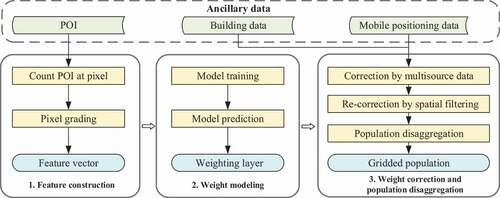
In step (1), feature vectors are constructed by grading pixels according to the number of POIs. In step (2), we input the constructed vectors as independent variables and population density as dependent variable to fit RF model at street-level for predicting population weights at pixel-level. In step (3), the weighting layer is corrected and recorrected based on multi-source data and spatial filtering, respectively; then it is used for population disaggregation from districts to pixels. Step (1) and (3) are the key steps of the proposed method and will be introduced in detail as follows.

3.1. Cross-scale feature construction (CSFC)

To address the scale mismatch problem in downscaling, the grade proportions of pixel-level attributes are constructed as feature vectors. Quantitative relation between graded POIs and population can distinguish the difference in population densities (Peng et al. 2020), so we use POIs as the pixel-level attributes for representing fine-grained population distribution. The illustration of feature construction method is shown in Figure 2. First, the study area is divided into pixels, and then the number of POIs for each selected POI type in a pixel is counted. Second, pixels are graded into levels using Natural Breaks according to the counted POIs. Finally, feature vectors are constructed based on the grading results.

Figure 2. Illustration of cross-scale feature construction using POIs.

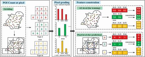
3.1.1. POI-based pixel grading

Pixel grading is carried on according to the counts of POIs for all pixels in study area, as shown in Figure 2. For each type of POIs, $L+1$ levels are set. To better reflect differences in population density for pixels with POIs, we adopt Natural Breaks to split a range of numbers into contiguous $L$ levels. Because it can minimize the squared deviation within each level by picking the level breaks that best group similar values (Chen et al. 2013). Meanwhile, a separated level of zero is assigned to the pixels without POIs (i.e. empty pixels).

3.1.2. Constructing feature vector of pixel grade proportions

Based on the grading results, feature vectors at AU-level (i.e. street-level) and pixel-level for training and prediction are constructed accordingly.

At street-level, we calculate the pixel proportions of each grading level and construct a $m\times \left(L+1\right)$ -dimensional feature vector for each street as Equation (1)(1) ${\beta }_i=\left[\begin{array}{c}{N}_i^{1,0},\dots ,N_i^{1,L},N_i^{2,0},\dots ,N_i^{2,L},\\ \dots ,N_i^{t,l},\dots ,N_i^{m,0},\dots ,N_i^{m,L}\end{array}\right]/N_i\left(0\le l\le L\right)$(1) :

(1) ${\beta }_i=\left[\begin{array}{c}{N}_i^{1,0},\dots ,N_i^{1,L},N_i^{2,0},\dots ,N_i^{2,L},\\ \dots ,N_i^{t,l},\dots ,N_i^{m,0},\dots ,N_i^{m,L}\end{array}\right]/N_i\left(0\le l\le L\right)$(1)

where ${\beta }_i$ is the feature vector for street $i$, $N_i$ is the total number of pixels of street $i$, $N_i^{t,l}$ is the number of pixels belonging to grading level $l$ for POI type $t$, and $m$ is the number of types of POIs.

At pixel-level, the constructed feature is also $m\times \left(L+1\right)$ -dimensional but a binary vector as Equation (2)(2) ${\alpha }_j=\left[\begin{array}{c}{B}_j^{1,0},\dots ,B_j^{1,L},B_j^{2,0},\dots ,B_j^{2,L}\\ ,\dots ,B_j^{t,l},\dots ,B_j^{m,0},\dots ,B_j^{m,L}\end{array}\right]\left(0\le l\le L\right)$(2) :

(2) ${\alpha }_j=\left[\begin{array}{c}{B}_j^{1,0},\dots ,B_j^{1,L},B_j^{2,0},\dots ,B_j^{2,L}\\ ,\dots ,B_j^{t,l},\dots ,B_j^{m,0},\dots ,B_j^{m,L}\end{array}\right]\left(0\le l\le L\right)$(2)

where ${\alpha }_j$ is the feature vector for pixel $j$, $B_j^{t,l}$ is 1 if pixel $j$ belongs to grading level $l$ for POI type $t$, otherwise it is 0. Although the data type of the feature vector entries at pixel-level differs from that at AU-level, 0 or 1 in each entry represents the proportion of pixel grades in each statistical unit as well. Compared with traditional feature construction method, statistical characteristic in CSFC is in the form of pixel proportions, and its differences and bimodality distribution (Sinha et al. 2019) will not be easily averaged out at AU-level. Therefore, the quantitative relation that how each grade contributes to population density is less affected by scale mismatch and can be transferred in cross-scale modeling.

3.2. Weight correction and population disaggregation

3.2.1. Weight correction based on multi-source data

Weight correction by utilizing multi-source data is indispensable. Although population is more concentrated around POIs, this relation is not linear. POI data have fine-grained location and rich semantics of urban facilities, but it might lead to bias as the spatial distribution of population is affected by multiple factors, such as residential conditions, surrounding environments and so on (Dong, Yang, and Cai 2016b; Bai, Wang, and Yang 2013). Therefore, building patch and mobile positioning data are employed to correct the initial weighting layer. The flow of weight correction is shown as Figure 3.

Figure 3. Flow of weight correction based on multi-source data.

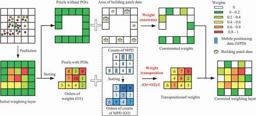
1. Weight Constraint (WC) based on building patch data

Building data constrain the spatial coverage of resident population and is helpful to describe the details of urban population (Dong, Yang, and Cai 2016a). Unlike linear regression model, which can set constant term to 0, RF assigns a non-zero weight value to all empty pixels. In that case, all empty pixels are considered to be inhabited and undifferentiated, which leads to prediction bias. In fact, empty pixels without buildings can be recognized uninhabited, while those with buildings might have different population size. As the area of building patch can be considered to have a proportional relation with population (Dong, Yang, and Cai 2016a), it can be utilized to constrain the weights of these pixels.

We set the population weights of the empty pixels without building patch data to 0, and differentiate the weights of the rest pixels according to the area of building patches. The formula is shown as Equation (3)(3) $w_j=w_{no\mathrm{\_}poi}\times {\left(\frac{are{a}_j}{are{a}_{max}}\right)}^{\theta }\times \gamma$(3) ..

(3) $w_j=w_{no\mathrm{\_}poi}\times {\left(\frac{are{a}_j}{are{a}_{max}}\right)}^{\theta }\times \gamma$(3)

where $w_{no\mathrm{\_}poi}$ is the uniform non-zero weight value assigned by RF model for empty pixels, $w_j$ is the weight after correction, $are{a}_j$ is the building patch area of pixel $j$, $are{a}_{max}$ is the largest building patch area of all empty pixels. $\theta$ is the exponential representing proportional relationship between population and area of building patch data, and $\gamma$ denotes the coefficient which stretches and limits the extent of corrected weights.

• (2) Weight Transposition (WT) based on mobile positioning data

As mobile positioning data reflect human activities at a specific moment, it can be used to balance the prediction bias by selecting the sample data within a certain time period. For better represent the spatial distribution of resident population, we select mobile positioning data from midnight period (detailed in Section 4.1.2) when most people stay at home.

Population weights represent the relative population density between pixels rather than the absolute population amounts. Due to incomplete and biased population coverage, the absolute and relative amounts of mobile users between pixels may differ from real-world situation; while the relative order of amounts is more reliable and stable, which can be utilized to adjust the order of population weights (i.e. the transposition of the population weights between the pixels). Original population weights and the amounts of mobile positioning users are sorted, respectively, into array $W$ and $M$ in ascending order, and the formula of weight transposition is shown in Equations (4)(4) $w_j=W_{inde{x}_j}$(4) ..

$inde{x}_j=\left(index\mathrm{\_}or{i}_j+index\mathrm{\_}mp{d}_j\right)\times 0.5$

(4) $w_j=W_{inde{x}_j}$(4)

where $index\mathrm{\_}or{i}_j$ is original index of the weight of pixel $j$ in the array $W$, $index\mathrm{\_}mp{d}_j$ is the index of pixel $j$ in array $M$, $inde{x}_j$ is the new index of the weight of pixel $j$ in array $W$ and $w_j$ is the new population weight of pixel $j$.

3.2.2. Spatial filtering for weight recorrection

The spatial distribution of population is continuous, smooth, and with the nature of spatial autocorrelation (Du, Zhang, and Zhang 2007; Gao et al. 2019). The population in a pixel not only rely on the statistical characteristics of the pixel itself but also affected by that of its neighboring pixels. However, pixel weights obtained from regression and correction using discrete POIs, building patch and mobile positioning data might lead to patchiness and discretization of population, which may contradict to real-world distribution. Learning from image smoothing in digital image processing (Banham and Katsaggelos 1997), we adopt spatial filtering to model the spatial autocorrelation in adjacent space. Gaussian filter template is selected considering that spatial influence of population decrease with distance (Peng et al. 2020) and approximately follows the Gaussian normal distribution (Chen 2000).

For each pixel $\left(x,y\right)$, we perform a convolution operation on a certain neighborhood of the pixel $\left(x,y\right)$, and assign the recorrected population weight to it. Assuming the size of filtering template is odd (i.e. $A=2\times a+1$), the recorrected population weight $g\left(x,y\right)$ is calculated as Equation (5)(5) $g\left(x,y\right)=\sum _{dx=-a}^{dx=a}\sum _{dy=-a}^{dy=a}w\left(a+1+dx,a+1+dy\right)\times f\left(x+dx,y+dy\right)$(5) ..

(5) $g\left(x,y\right)=\sum _{dx=-a}^{dx=a}\sum _{dy=-a}^{dy=a}w\left(a+1+dx,a+1+dy\right)\times f\left(x+dx,y+dy\right)$(5)

where $w\left(a+1+dx,a+1+dy\right)$ is the weight of cell $\left(a+1+dx,a+1+dy\right)$ in the filter template, $f\left(x+s,y+t\right)$ is the original population weight of pixel $\left(x+dx,y+dy\right)$.

3.2.3. Population disaggregation

After weight recorrection, census population can be disaggregated from districts to pixels with the generated weighting layer using Equation (6)(6) $PO{P}_{pixel\mathrm{\_}j}=PO{P}_{district\mathrm{\_}k}\times \frac{w_{pixel\mathrm{\_}j}}{w_{district\mathrm{\_}k}}$(6) :

(6) $PO{P}_{pixel\mathrm{\_}j}=PO{P}_{district\mathrm{\_}k}\times \frac{w_{pixel\mathrm{\_}j}}{w_{district\mathrm{\_}k}}$(6)

where $w_{pixel\mathrm{\_}j}$ is the population weight for pixel $j$, $w_{district\mathrm{\_}k}$ represents the summed population weight of all pixels in district $k$ that pixel $j$ belongs to, $PO{P}_{district\mathrm{\_}k}$ is the census population of district $k$, and $PO{P}_{pixel\mathrm{\_}j}$ represents the predicted population of pixel $j$.

4. Experiments and analysis

4.1. Experimental Setting

Experiments were designed to validate the effectiveness of the cross-scale feature construction and each weight correcting step. In section 4.2, the impact of grading level amounts on population estimation accuracy was discussed, and CSFC was validated by comparing with traditional feature construction method followed by the variable importance analysis on population weights for different POI types. The effectiveness of weight correction was examined by comparing with traditional data fusion method in Section 4.3. To evaluate the effects of spatial filtering, we explored the influence of pixel resolution, region and template size in Section 4.4. Overall accuracy was assessed through a comparison with WorldPop and GPW, and errors of population spatialization were visualized and analyzed in Section 4.5.

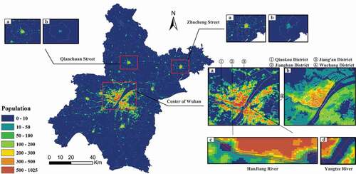
4.1.1. Study area

Wuhan, the capital city of Hubei Province, China (Figure 4(a), is selected as the study area. It is located in the east of Jianghan Plain and the middle reaches of Yangtze River. The geographic extent is 29°58′ to 31°22′ N and 113°41′ to 115°05′ E. In 2015, the resident population was about 10.607 million, accounting for 18.13% of the total population of Hubei Province. The city consists of 13 districts, which are divided into 186 streets. Among the 13 districts as shown in Figure 4(b), there are 7 central districts (account for 61.67% of total population) and 6 suburban districts (account for 38.33% of total population). Wuhan extends over areas with high and low population densities, and the population distribution patterns are complex, which makes Wuhan a suitable experimental area for validating the effectiveness and robustness of the proposed population spatialization method.

Figure 4. Overview of the study area Wuhan. (a) Location of Wuhan in Hubei Province. (b) Spatial distribution of 13 districts. (c) Spatial distribution of 186 streets with high, medium, and low population densities, respectively.

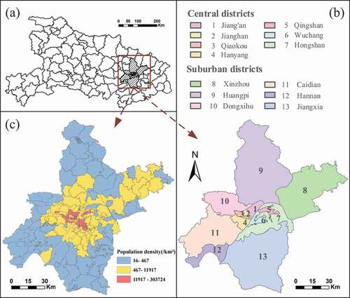
To better evaluate effects of the proposed method in different population density regions, we divide Wuhan streets into high, medium and low population density levels using Natural Breaks. The result of density grading of 186 streets is shown in Figure 4(c), among which there are 57, 69, and 60 streets with high, medium, and low population densities, respectively. It can be seen that most of the high-density streets are located in main urban area, while low-density streets are mainly located in suburban area.

4.1.2. Experimental data

POIs, building patch, mobile positioning, census population, WorldPop, and GPW data were used in this study as experimental data (Table 1). All spatial references of these data were unified to WGS-84. The acquisition and preprocessing of these data in the current study are described below.

Table 1. Type, year, and source of experimental data.

Dataset		Year	Source
Ancillary data	POIs	2017	Gaode Map Services, China (https://www.amap.com/)
	Building patch data	2015	National Geoinformation Survey
	Mobile positioning data	2018	Wayz.AI
Reference data	Census population data	2015	Wuhan Statistical Yearbook, Wuhan Community Demographic Census
	WorldPop dataset	2015	WorldPop Mainland China dataset for 2015 (http://www.worldpop.org.uk/)
	GPW v4 dataset	2015	Socioeconomic Data and Applications Center (http://srtm.csi.cgiar.org)

The POI data was retrieved from Gaode Map, which is one of the most popular commercial map services in China. After removal of types with few and incomplete records, twelve types of POIs, which are highly correlated with population distribution, were selected, as shown in Table 2. Building patch data was obtained from National Geoinformation Survey, in which the patches with area less than 200 m² were not included. Two months (April to May, Year 2018) of desensitized mobile positioning data was collected from Wayz.AI, a location-based service company who provides positioning function for various Apps. We excluded holidays, weekends, and the days with incomplete data and randomly selected 4 days data that contains 266,460 mobile users, accounting for 2.7% of the total population of Wuhan. Then we generated grid-based statistics of the amounts of mobile users in the midnight period (from 11:00 pm to 3:00 am) with 500 m, 200 m, and 100 m spatial resolutions, respectively. The district-level and street-level census data were obtained from the Wuhan Statistical Yearbook in 2015 and the Wuhan Community Demographic Census in 2015, respectively. The WorldPop and GPW dataset were obtained from the WorldPop project and Socioeconomic Data and Applications Center, respectively, which are chosen as validation data in accuracy assessments.

Table 2. Types and counts of the selected POIs in experiments.

Type	Count	Type	Count
Research and education	6640	Hospital	3864
Medical service	6357	Shopping	42,014
Financial services	4689	Accommodation	3564
Restaurant	13,900	Residential community	11,279
Leisure and entertainment	5273	Government agency	9618
Parking lot	3460	Auto service	5716

4.1.3. Model parameters

Random forest model is implemented using python Sklearn library. The main parameters of RF model are set to the following: (1) n_estimators = 250, (2) max_features = sqrt and (3) min_samples_leaf = 1. The term n_estimators represents the number of decision trees, the larger n_estimators is, the better the RF performs. As the number of trees increases, the computing time increases accordingly. 250 is the trade-off of training time and accuracy. The term max_features is the number of subsets of the randomly selected feature set. The fewer the number of subsets, the faster the variance decreases, but the deviation increases. The term min_samples_leaf represents the minimum sample leaf node number. The parameter values of sqrt and 1 are selected after tuning parameters.

4.1.4. Evaluation metrics

Since there are no real pixel-level population dataset, validation is conducted by comparing the aggregated predicted population with census counts for each street (Sinha et al. 2019). We perform experiments at 100 m, 200 m, and 500 m spatial resolutions, respectively. The street-level accuracy evaluation indexes include the Mean Absolute Error (MAE), the Root Mean Square Error (RMSE), and coefficient of determination (R²), which are calculated as Equation (7)(7) $RMSE=\sqrt{\frac{1}{n}\sum _{i=1}^n{\left(Predic{t}_i-Rea{l}_i\right)}^2}$(7) :

$MAE=\frac{1}{n}\sum _{i=1}^n\left|Predic{t}_i-Rea{l}_i\right|$

(7) $RMSE=\sqrt{\frac{1}{n}\sum _{i=1}^n{\left(Predic{t}_i-Rea{l}_i\right)}^2}$(7)

$R^2=1-\frac{{\sum }_i{\left(Rea{l}_i-Predic{t}_i\right)}^2}{{\sum }_i{\left(Rea{l}_i-\overline{Real}\right)}^2}$

where $Predic{t}_i$ represents the predicted population of street $i$, $Rea{l}_i$ represents census counts of street $i$,$\overline{Real}$ is the average population of all streets and $n$ is the total number of streets.

4.2. Validation of cross-scale feature construction method

4.2.1. Impact of the number of grading levels

As pixels of different grading levels represent different population densities, dividing appropriate levels is crucial for feature construction. This experiment aims to select an appropriate number of grading levels for conducting subsequent experiments and investigate how the results change under different grading levels. Thus, we vary the numbers of grading levels from 2 to 8, i.e. the non-empty pixel grades divided by Natural Breaks ranging from 1 to 7. The results are presented in Figure 5.

Figure 5. Accuracy comparison under an increasing numbers of grading levels at 500 m, 200 m, and 100 m resolutions, respectively.

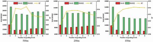
As shown in Figure 5, accuracies display different trends under an increasing numbers of grading levels at different resolutions, and there is no global optimal number of grading levels. The accuracy is lowest when the number of grading levels is 2 for all three resolutions, possibly because the pixels are only graded according to whether containing POIs or not, neglecting the quantity information of POIs. At 500 m and 200 m resolutions, the accuracy is higher when the number of grading levels is small in general. While at 100 m resolution, accuracy increases first until the number of grading levels reaches a certain threshold. Small pixels with fine resolution (e.g. 100 m) contain less types and counts of POIs, where subtle attribute differences might indicate a distinctly different attraction degree to population. Thus more levels are needed to capture these differences in grades. We can also find that the accuracy is relatively high when the number of grading levels is 5 at all three resolutions. Thereby the number of grading levels is set to 5 in the following experiments.

4.2.2. Comparison of feature construction method

To validate the effectiveness of CSFC, we compare its accuracy with Traditional Feature Construction (TFC) method, as shown in Figure 6. TFC builds POI-density index and inputs POI density as independent variables for model training and prediction. To eliminate the influence of weight adjustment on the result, we remove the steps of weight correction and recorrection, and the initial weighting layer obtained from RF is directly used for population disaggregation.

Figure 6. Accuracy comparison between CSFC method and TFC method. (a) The result at 500 m, 200 m and 100 m resolution, respectively. (b)-(c) Scatterplots of the predicted and the census population density at the street-level at 100 m resolution. A log10-log10 transformation was conducted for the population density. The red, green, and blue points represent high, medium, and low population density streets, while red, green, and blue line are fitting lines, respectively. The black dash line is the global fitting line.

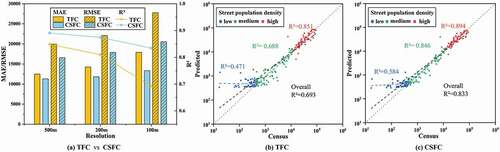
Figure 6 manifests that CSFC can alleviate the scale mismatch problem in downscaling and improve the accuracy of population spatialization. As shown in Figure 6(a), when the spatial resolution getting higher, the accuracy of both methods decreased. Nonetheless, the proposed method is less affected when significant scale differences exist between training and prediction. Figure 6(b,c) shows the fitting results between predicted and census population density in which each scatter point corresponds to a street. A match of 100% would be visible as a straight diagonal line. CSFC has similar distribution pattern of scatter points with TFC, but scatter points are more convergent to the diagonal line. In many cases, POI-density-based models suffer from underestimation of population in main urban areas and overestimation in rural areas (Wang, Fan, and Wang 2020). It leads to that blue points are mainly above the diagonal line, while red and green points are mostly distributed below the line. According to the comparison of R² between CSFC and TFC, we can find that accuracies in low- and medium-density streets are effectively improved, which means that CSFC can ameliorate the overestimation and underestimation in several extreme population density regions to some extent. However, as there are many empty pixels without POIs are assigned a non-zero population weight by RF model, the severe overestimation of population still exists in rural areas (blue points). Therefore, it is necessary to further correct the prediction errors by integrating multi-source data.

4.2.3. Variable importance analysis on population weights for different POI types

As different types of POIs have different levels of correlation with population density, the analysis of feature importance helps to understand how POIs impact on population weights, and in turn better explain the influencing mechanism of different POI types on population distribution. To achieve this goal, we extract estimated importance of all input variables from RF model established upon Sklearn, a Python-based machine learning library, using built-in application Programming Interface (API) “RandomForestRegressor.feature_importances_”. The variables importance for RF regression in our population estimation task is shown in Figure 7.

Figure 7. Variables importance for RF regression. The blue heatmap represents variables importance of 5 grading levels where the number of POIs in the pixel is from less to more accordingly for each POI type, while red heatmap represents the sum of variables importance of 5 grading levels.

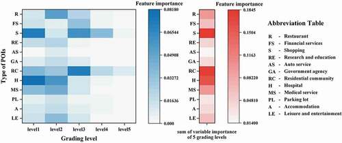
Figure 7 displays variables importance of 5 grading levels and its sum, respectively, for each POI type. It can be found that hospital (H), shopping (S), and residential community (RC) are highly correlated with population weights and followed by medical service (MS) and restaurant (R), while auto service (AS), commercial parking lot (PL), government agency (GA), and accommodation (A) have less impact on that. These observations are in line with our common sense. While the importance of financial service (FS), and leisure and entertainment (LE) are in between them, because these facilities also link with our daily life, but may have less revisiting frequency than shopping and restaurant. Research and education (RE) is less important than financial service but more than auto service etc., probably because this type of POI contains high schools and universities that with large number of resident students inside, as well as scientific research institutions, which don’t contribute to residential population. Meanwhile, we can also find that variables at low-level play more important roles in RF regression in general, since high-density level pixels only account for small proportions. More specifically, for POI types such as hospital, medical service and research education, the first two levels are significantly more important than the other levels, because presence or absence of such POIs matters, which determines whether population residence forms nearby. While for POI types like shopping and residential community, each level has a certain degree of importance, which shows that the number of such types of POIs is directly correlated to the population, and these POIs are more likely concentrated and thus forming more density levels and spatial agglomerations.

4.3. Effectiveness of weight correction based on multi-source data

Based on initial weighting layer, weight constraint and weight transposition are conducted sequentially. In this experiment, we compare the accuracy of the proposed weight correction method with traditional data fusion method, i.e. so-called Input Variable Method (IVM) in this paper, which input statistics of the amounts of mobile users and area of building patch as covariates for regression directly. The results are presented in Figure 8.

Figure 8. Accuracy comparison between weight correction method and traditional data fusion method (IVM). CSFC+WC represents the building patch data is used for Weight Constraint (WC) to correct the initial population weighting layer obtained from modeling based on CSFC, CSFC+WC+WT represents the further utilization of mobile positioning data for Weight Transposition (WT). (a) The result at 500 m, 200 m, and 100 m resolution, respectively. (b)-(c) Scatterplots of the predicted and the census population density at the street-level at 100 m resolution.

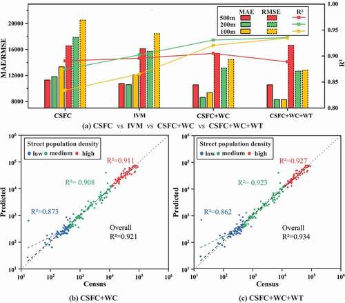
Figure 8 illustrates weight correction method outperforms IVM, although incorporating more data as input variables for regression improves accuracy as well. As shown in Figure 8(a), weight correction method has a better accuracy improvement at fine resolution than at coarse resolution. However, according to R² and RMSE, we can find that WT reduces the accuracy when the spatial resolution is 500 m. It might be because large pixels with coarse resolution contain more types of POIs with abundant semantic information, which will not cause severe misestimation of population in commercial zones and residential areas; while biased population coverage of mobile positioning data increases the errors. Comparing with Figure 6(c), the overestimation of population in low-density streets is significantly corrected in Figure 8(b), because population weight of the pixels without building patch data is set to 0. Besides, since weights are transposed between the pixels with POIs, which are mainly distributed in main urban areas, accuracies in high-density and medium-density streets are further improved (Figure 8(c)). In general, WC corrects the overestimation problem of low population density regions, while WT refines the population distribution in high population density regions.

4.4. Effects of spatial filtering for weight recorrection

To find the optimal distance to perform spatial filtering, we compare the accuracy at three pixel resolutions by varying the size of Gaussian filter templates, as shown in Figure 9. In this experiment, filtering is performed in central districts, suburban districts and entire Wuhan, respectively, to explore the effect of region on the results.

Figure 9. Accuracy comparison under different sizes of filtering template and different regions at 500 m, 200 m, and 100 m resolutions, respectively.

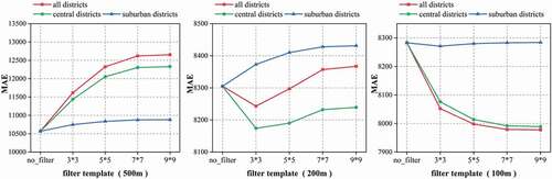
The results in Figure 9 indicate that spatial filtering can improve the accuracy of population spatialization at fine resolution but have an opposite effect at coarse resolution. At 500 m resolution, accuracy decreases after performing spatial filtering. At 200 m resolution, filtering with small template size is effective, but with large size increases errors. While at 100 m resolution, accuracy increases first and then slows down its upward trend. In general, the performance of spatial filtering become less effective and even worse as the size of filtering template continuously increases. By observing the effect of different sizes of filtering template on the results for all three resolutions, it can be found that the optimal distance to perform spatial filtering is about 600 m. From the perspective of the spatial distribution, it will be more useful to perform spatial filtering in central districts rather than suburban districts because of the close and strong spatial association between population inside urban city. Therefore, spatial filtering is recommended for fine-resolution population spatialization in central urban areas.

4.5. Accuracy assessment and agreement analysis

WorldPop and GPW are used as benchmarks to evaluate the accuracy of the proposed method. Meanwhile, we made a comparison with a RF based model (Ye et al. 2019). Ye’s model uses POI, road networks, NDVI, elevation, slope and NTL to form the relationship between population distribution and multi-source data. Table 3 lists accuracies of GPW, WorldPop, Ye’s model and the proposed method at different resolutions. On the whole, our method has a higher overall accuracy. The best accuracy of our method is achieved at 100 resolution as demonstrated by MAE, which is about one-sixth, one-third and half of GPW, WorldPop and Ye’s model, respectively. Although the accuracy decreases with resolution getting lower, our method still outperforms other datasets and methods. We can find that, with the help of fine-grained ancillary data and CSFC, the proposed method is more likely to be adopted in population spatialization scenario with fine-resolution.

Table 3. Accuracies of GPW, WorldPop, Ye’s model and the proposed method at 500 m, 200 m, and 100 m resolutions, respectively.

Dataset/Method	Resolution (m)	MAE	RMSE	R^2
GPW	1000	46,919	81,077	0.49
WorldPop	100	23,763	40,500	0.55
Ye’s model	100	16,922	25,259	0.74
	200	15,451	23,181	0.78
	500	14,581	21,744	0.81
Proposed method	100	7992	12,365	0.939
	200	8174	12,502	0.937
	500	10,569	16,653	0.887

Figure 10 exhibits the population spatialization results of our method at 100 m resolution and WorldPop dataset in whole city of Wuhan and selected regions. They share a similar spatial pattern of population, but are visually different in details. It is found that population is mainly distributed in the central area of Wuhan (i.e. Jiang’an District, Jianghan District, Qiaokou District and Wuchang District) in both results, while our method can identify high-density nuclei of population in the periphery, such as Qianchuan street and Zhucheng street. From Figure 10(a,b), we can also find WorldPop is difficult to depict sporadic population distribution, while our method can better capture these details as fine-grained POIs are incorporated for modeling. Meanwhile, the result of the WorldPop follow the similar spatial patterns of the contours of land patches, which present a wide coverage but homogeneous spatial distribution of population, and has clear boundaries around water body. In contrast, the proposed method depicts a higher density mapping of population clustered around POIs, which has more obvious graininess and prominent texture. It reveals the spatial heterogeneity of population distribution within statistical district, and better present the details of population distribution. However, spatial filtering leads to slight spillover of population at boundary of water body (Figure 10(c,d)), which especially has great impact on small river and lakes (e.g. Hanjiang River) as the population of pixels dropped into a narrow river might be affected by neighbor pixels located outside the water body from multiple directions. By incorporating water body data, such errors could be eliminated furtherly.

Figure 10. Population spatialization results of our method at 100 m resolution and WorldPop dataset. For each amplified subregion, subgraphs (a) and (b) represents our results and WorldPop, respectively, while subgraphs (c) and (d) show the vector boundaries of Hangjiang River and Yangtze River in our results.

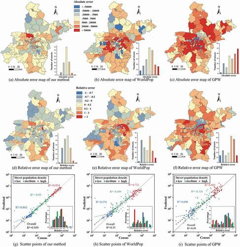
Accuracy assessments and agreement analysis with WorldPop and GPW are conducted furtherly by evaluating absolute and relative errors at street-level (Figure 11). As shown in absolute error maps (Figure 11(a–c)), our method has lower errors in high-, medium-, and low-density streets compared to WorldPop and GPW. From the statistical histograms in the right-bottom of Figure 11(a–c), we can find that the numbers of overestimated and underestimated streets are roughly equal in our method and WorldPop, while GPW overestimates population in most streets. This is because census counts are redistributed from AU-level to pixel-level in our method and WorldPop, but GPW interpolates population directly according to overlapping area. In relative error maps (Figure 11(d–f)), the streets with low predicted error (from −0.2 to 0.2) of our method account for 61% of the total number of streets, whereas those of WorldPop and GPW are 29% and 18%, respectively. Figure 11(g–i) show that scatter points for the predicted population in all streets of our method are concentrated on both sides of the diagonal line, while those of WorldPop and GPW are more discrete. R² of our method is 0.939, around 1.7 times and 1.9 times those of WorldPop and GPW, respectively, which demonstrates our method can better fit the real population distribution. As WorldPop presents a more homogeneous population distribution, it leads to underestimation in high-density streets (red points) and overestimation in low-density streets (blue points). Scatter points of GPW have greater discretization and its errors are mainly derived from overestimation in most streets. Meanwhile, from the percentage histograms of the relative error (detailed in Table A1 in Appendix), it can be seen that the errors of our method are normally distributed and more balanced in general, i.e. with more streets located in low relative error ranges and less streets in high error ranges. However, for low-density streets, this observation is not hold. A few streets are significantly overestimated and make the corresponding scatter points deviate from the diagonal line, which indicates that our method suffers from accuracy problem in rural areas like many other POI-based studies (Wang, Fan, and Wang 2020). Nonetheless, R² of low-density streets is 0.865, lower than 0.93 in medium and 0.934 in high-density streets, it has achieved significant improvement after weight correction and performs much better than WorldPop and GPW.

Figure 11. Accuracy comparison between our method, WorldPop and GPW at street-level. (a) -(c) Absolute error maps and accuracy histograms. (d)-(f) Relative error maps and accuracy histograms. (g)-(i) Scatterplots of the predicted and the census population density, and percentage histograms of the relative error.

5. Conclusion and future work

This paper proposed a cross-scale method of population spatialization based on RF. Specifically, by considering pixel-level grading of POI counts, CSFC partially overcomes the scale mismatch problem in downscaling. Comparing with traditional feature construction method, CSFC can achieve relatively high accuracy especially when significant scale differences exist between inputs of training and prediction (i.e. AU-level and pixel-level). Additionally, by integrating multiple fine-grained ancillary data to correct population weight and using spatial filtering to model the autocorrelation of population distribution, the accuracy can be further improved. Through comparisons, our results showed higher estimation accuracy than WorldPop dataset. Therefore, the proposed method can be used for fine-resolution population estimation. Furthermore, it could provide insights on spatial downscaling modeling scenarios for disaggregating aggregated counts to a finer scale.

It should be pointed out that there is still much space for improvement. Future work would focus on the following directions. First, we can further study the adaptive cross-scale population spatialization method. An adaptive rule should be adopted to determine the number of grading levels according to the attribute characteristics of different modeling data. Besides, adaptive kernel density estimation algorithm (Yuan et al. 2019) could be used for reference to choose filter template size. Second, multi-source data such as building patch and mobile positioning data are mainly for weight correction in this study, which is the rule we set manually based on prior knowledge and not integrated into the machine learning model in a data-driven way. Meanwhile, our method suffers from overestimation in rural areas. Better feature modeling methods, as well as more data types remain to be explored to address these problems. Finally, many geographic features (e.g. water body, bridges, viaducts) in a city might influence the spatial connectivity and interaction, but spatial filtering based on Euclidean distance cannot depict such effects appropriately. In the future, we can design a non-Euclidean spatial filter or adopt spatial context modeling using representation learning (Yao et al. 2017; Liu, Andris, and Rahimi 2019) to model the connectivity of population and spatial relations between ancillary data.

Disclosure statement

No potential conflict of interest was reported by the author(s).

Data availability statement

The code and data that support the findings of this study are openly available in GitHub at https://github.com/ZPGuiGroupWhu/PopulationSpatialization

Additional information

Funding

This paper is supported by National Natural Science Foundation of China [Grant Nos. 42090010, U20A2091, 41971349, and 41930107] and National Key R&D Program of China [Grant Nos. 2018YFC0809800 and 2017YFB0503704].

Notes on contributors

Yuao Mei

Yuao Mei is a master student in the School of Remote Sensing and Information Engineering, Wuhan University. His research interests are population spatialization and spatiotemporal data analysis.

Zhipeng Gui

Zhipeng Gui is an Associate Professor in the School of Remote Sensing and Information Engineering, Wuhan University. His research interests include geospatial artificial intelligence, spatiotemporal data analysis and high-performance geocomputation.

Jinghang Wu

Jinghang Wu received his master’s degree from the School of Remote Sensing and Information Engineering, Wuhan University. His research interests are population spatialization and high-performance geocomputation.

Dehua Peng

Dehua Peng is a PhD student in the State Key Laboratory of Information Engineering in Surveying, Mapping and Remote Sensing, Wuhan University. His research interests are clustering algorithms and point pattern mining.

Rui Li

Rui Li is a full Professor in the State Key Laboratory of Information Engineering in Surveying, Mapping and Remote Sensing, Wuhan University. Her research interests are networking communication, spatial-temporal computing, and networks GIS.

Huayi Wu

Huayi Wu is a full Professor in the State Key Laboratory of Information Engineering in Surveying, Mapping and Remote Sensing, Wuhan University. His research interests are high-performance geospatial computing and intelligent geospatial web services.

Zhengyang Wei

Zhengyang Wei received her bachelor’s degree from the School of Remote Sensing and Information Engineering, Wuhan University. She is now pursuing her master degree in Stanford Unversity. Her research interests are text classification and computer vision.

Appendix

Table A1. The number and proportion of streets under different relative error ranges for three density levels.

Method/dataset	Relative Error range	Number and proportion of streets for three density levels
		Low-density	Medium-density	High-density
Our method	−1 – −0.7	0 (0%)	0 (0%)	1 (1.7%)
	−0.7- −0.2	10 (16.6%)	12 (17.3%)	11 (19.3%)
	−0.2 – 0	15 (25%)	26 (37.6%)	12 (21%)
	0 – 0.2	16 (26.6%)	29 (42%)	25 (43.8%)
	0.2 – 1	15 (25%)	9 (13%)	8 (14%)
	1 – 3	3 (5%)	1 (1.4%)	0 (0%)
	> 3	1 (1.6%)	1 (1.4%)	0 (0%)
WorldPop	−1 – −0.7	0 (0%)	1 (1.4%)	1 (1.7%)
	−0.7- −0.2	6 (10.2%)	10 (14.5%)	29 (50.9%)
	−0.2 – 0	6 (10.2%)	10 (14.5%)	14 (24.6%)
	0 – 0.2	7 (11.9%)	11 (15.9%)	6 (10.5%)
	0.2 – 1	25 (42.4%)	20 (29%)	7 (12.3%)
	1 – 3	10 (16.9%)	13 (18.8%)	0 (0%)
	> 3	5 (8.5%)	4 (5.8%)	0 (0%)
GPW	−1 – −0.7	0 (0%)	5 (7.2%)	10 (17.5%)
	−0.7- −0.2	4 (6.8%)	10 (14.5%)	10 (17.5%)
	−0.2 – 0	6 (10.2%)	4 (5.8%)	4 (7%)
	0 – 0.2	8 (13.6%)	5 (7.2%)	6 (10.5%)
	0.2 – 1	17 (28.9%)	21 (30.4%)	15 (26.3%)
	1 – 3	20 (33.9%)	16 (23.2%)	11 (19.3%)
	> 3	5 (8.5%)	8 (11.6%)	1(1.7%)

References

- Ahola, T., K. Virrantaus, J.M. Krisp, and G.J. Hunter. 2007. “A Spatio-temporal Population Model to Support Risk Assessment and Damage Analysis for Decision-making.” International Journal of Geographical Information Science 21 (8): 935–953. doi:10.1080/13658810701349078.
- Aubrecht, C., R. Gunasekera, J. Ungar, and O. Ishizawa. 2016. “Consistent yet Adaptive Global Geospatial Identification of Urban-rural Patterns: The iURBAN Model.” Remote Sensing of Environment 187 (15): 230–240. doi:10.1016/j.rse.2016.10.031.
- Bachir, D., V. Gauthier, M. El Yacoubi, and G. Khodabandelou. 2017. “Using Mobile Phone Data Analysis for the Estimation of Daily Urban Dynamics.” In 2017 IEEE 20th international conference on intelligent transportation systems (ITSC), Yokohama, Japan, October 16-19.
- Bai, Z., J. Wang, H. Jiang, and M. Gao. 2015. “The Gridding Approach to Redistribute Population Based on Multi-source Data.” Journal of Geo-Information Science 17 (6): 653–660. doi:10.3724/SP.J.1047.2015.0065.
- Bai, Z., J. Wang, and F. Yang. 2013. “Research Progress in Spatialization of Population Data.” Progress in Geography 32 (11): 1692–1702. doi:10.11820/dlkxjz.2013.11.012.
- Bakillah, M., S. Liang, A. Mobasheri, J. Jokar Arsanjani, and A. Zipf. 2014. “Fine-resolution Population Mapping Using OpenStreetMap Points-of-interest.” International Journal of Geographical Information Science 28 (9): 1940–1963. doi:10.1080/13658816.2014.909045.
- Banham, M.R., and A.K. Katsaggelos. 1997. “Digital Image Restoration.” IEEE Signal Processing Magazine 14 (2): 24–41. doi:10.1109/79.581363.
- Breiman, L. 1996. “Bagging Predictors.” Machine Learning 24 (2): 123–140. doi:10.1007/BF00058655.
- Breiman, L. 2001. “Random Forests.” Machine Learning 45 (1): 5–32. doi:10.1023/a:1010933404324.
- Brunsdon, C., S. Fotheringham, and M. Charlton. 1998. “Geographically Weighted Regression.” Journal of the Royal Statistical Society: Series D (The Statistician) 47 (3): 431–443. doi:10.1111/1467-9884.00145.
- Chen, J., S. Yang, H. Li, B. Zhang, and J. Lv. 2013. “Research on Geographical Environment Unit Division Based on the Method of Natural Breaks (Jenks).” International Archives of the Photogrammetry, Remote Sensing and Spatial Information Sciences XL-4/W3: 47–50. doi:10.5194/isprsarchives-XL-4-W3-47-2013.
- Chen, X. 2018. “A Spatial and Temporal Analysis of the Socioeconomic Factors Associated with Breast Cancer in Illinois Using Geographically Weighted Generalized Linear Regression.” Journal of Geovisualization and Spatial Analysis 2 (1): 1–16. doi:10.1007/s41651-017-0011-5.
- Chen, Y. 2000. “A Theoretical Proof of Clark’s Model on Spatial Distribution Density of Urban Population.” Journal of Xinyang Teachers College(Natural Science Edition) 13 (2): 185–188.
- Clark, C. 1951. “Urban Population Densities.” Journal of the Royal Statistical Society. Series A (General) 114 (4): 490–496. doi:10.2307/2981088.
- De Knegt, H., F. V. van Langevelde, M. Coughenour, A. Skidmore, W. De Boer, I. Heitkönig, N. Knox, R. Slotow, C. Van der Waal, and H. Prins. 2010. “Spatial Autocorrelation and the Scaling of Species–environment Relationships.” Ecology 91 (8): 2455–2465. doi:10.1890/09-1359.1.
- Deville, P., C. Linard, S. Martin, M. Gilbert, F.R. Stevens, A.E. Gaughan, V.D. Blondel, and A.J. Tatem. 2014. “Dynamic Population Mapping Using Mobile Phone Data.” Proceedings of the National Academy of Sciences 111 (45): 15888–15893. doi:10.1073/pnas.1408439111.
- Dong, N., X. Yang, and H. Cai. 2016a. “A Method for Demographic Data Spatialization Based on Residential Space Attributes.” Progress in Geography 35 (11): 1317–1328. doi:10.18306/dlkxjz.2016.11.002.
- Dong, N., X. Yang, and H. Cai. 2016b. “Research Progress and Perspective on the Spatialization of Population Data.” Journal of Geo-Information Science 18 (10): 1295–1304. doi:10.3724/SP.J.1047.2016.01295.
- Dong, N., X. Yang, H. Cai, and F. Xu. 2017. “Research on Grid Size Suitability of Gridded Population Distribution in Urban Area: A Case Study in Urban Area of Xuanzhou District, China.” PloS one 12 (1): e0170830. doi:10.1371/journal.pone.0170830.
- Dong, N., X. Yang, D. Huang, and D. Han. 2018. “Spatialization Method of Demographic Data Based on Urban Public Facility Elements.” Journal of Geo-Information Science 20 (7): 918–928. doi:10.12082/dqxxkx.2018.170625.
- Doupe, P., E. Bruzelius, J. Faghmous, and S.G. Ruchman. 2016. “Equitable Development through Deep Learning: The Case of Sub-national Population Density Estimation.” In Proceedings of the 7th Annual Symposium on Computing for Development, Nairobi, Kenya, November 18-20.
- Du, G., S. Zhang, and Y. Zhang. 2007. “Analyzing Spatial Auto-correlation of Population Distribution: A Case of Shenyang City.” Geographical Research 26 (2): 383–390. doi:10.11821/yj2007020020.
- Fan, Y., P. Shi, Z. Gu, and X. Li. 2004. “A Method of Data Gridding from Administration Cell to Gridding Cell.” Scientia Geographica Sinica 24 (1): 105–108. doi:10.13249/j.cnki.sgs.2004.01.105.
- Fecht, D., S. Cockings, S. Hodgson, F.B. Piel, D. Martin, and L.A. Waller. 2020. “Advances in Mapping Population and Demographic Characteristics at Small-area Levels.” International Journal of Epidemiology 49 (Supplement_1): i15–i25. doi:10.1093/ije/dyz179.
- Gao, S., K. Janowicz, and H. Couclelis. 2017. “Extracting Urban Functional Regions from Points of Interest and Human Activities on Location‐based Social Networks.” Transactions in GIS 21 (3): 446–467. doi:10.1111/tgis.12289.
- Gao, Y., J. Cheng, H. Meng, and Y. Liu. 2019. “Measuring Spatio-temporal Autocorrelation in Time Series Data of Collective Human Mobility.” Geo-spatial Information Science 22 (3): 166–173. doi:10.1080/10095020.2019.1643609.
- Goodchild, M.F., and -N.S.-N. Lam. 1980. “Areal Interpolation: A Variant of the Traditional Spatial Problem.” Geo-Processing 1 (3): 297–312. doi:10.1068/a121427.
- Jia, P., and A.E. Gaughan. 2016. “Dasymetric Modeling: A Hybrid Approach Using Land Cover and Tax Parcel Data for Mapping Population in Alachua County, Florida.” Applied Geography 66: 100–108. doi:10.1016/j.apgeog.2015.11.006.
- Leyk, S., A.E. Gaughan, S.B. Adamo, A. de Sherbinin, D. Balk, S. Freire, A. Rose, F.R. Stevens, B. Blankespoor, and C. Frye. 2019. “The Spatial Allocation of Population: A Review of Large-scale Gridded Population Data Products and Their Fitness for Use.” Earth System Science Data 11 (3): 1385–1409. doi:10.5194/essd-11-1385-2019.
- Li, F., Z. Gui, H. Wu, J. Gong, Y. Wang, S. Tian, and J. Zhang. 2018a. “Big Enterprise Registration Data Imputation: Supporting Spatiotemporal Analysis of Industries in China.” Computers, Environment and Urban Systems 70: 9–23. doi:10.1016/j.compenvurbsys.2018.01.010.
- Li, K., Y. Chen, and Y. Li. 2018. “The Random Forest-based Method of Fine-resolution Population Spatialization by Using the International Space Station Nighttime Photography and Social Sensing Data.” Remote Sensing 10 (10): 1650. doi:10.3390/rs10101650.
- Li, L., J. Li, Z. Jiang, L. Zhao, and P. Zhao. 2018b. “Methods of Population Spatialization Based on the Classification Information of Buildings from China’s First National Geoinformation Survey in Urban Area: A Case Study of Wuchang District, Wuhan City, China.” Sensors 18 (8): 2558. doi:10.3390/s18082558.
- Liu, X., C. Andris, and S. Rahimi. 2019. “Place Niche and Its Regional Variability: Measuring Spatial Context Patterns for Points of Interest with Representation Learning.” Computers, Environment and Urban Systems 75: 146–160. doi:10.1016/j.compenvurbsys.2019.01.011.
- Lo, C. 2008. “Population Estimation Using Geographically Weighted Regression.” GIScience & Remote Sensing 45 (2): 131–148. doi:10.2747/1548-1603.45.2.131.
- Lwin, K.K. 2010. “Online Micro-spatial Analysis Based on GIS Estimated Building Population: A Case of Tsukuba City.” Ph. D. in Science, University of Tsukuba.
- Mennis, J., and T. Hultgren. 2006. “Intelligent Dasymetric Mapping and Its Application to Areal Interpolation.” Cartography and Geographic Information Science 33 (3): 179–194. doi:10.1559/152304006779077309.
- Nagle, N.N., B.P. Buttenfield, S. Leyk, and S. Spielman. 2014. “Dasymetric Modeling and Uncertainty.” Annals of the Association of American Geographers 104 (1): 80–95. doi:10.1080/00045608.2013.843439.
- Patel, N.N., F.R. Stevens, Z. Huang, A.E. Gaughan, I. Elyazar, and A.J. Tatem. 2017. “Improving Large Area Population Mapping Using Geotweet Densities.” Transactions in GIS 21 (2): 317–331. doi:10.1111/tgis.12214.
- Peng, Z., R. Wang, L. Liu, and H. Wu. 2020. “Fine-Scale Dasymetric Population Mapping with Mobile Phone and Building Use Data Based on Grid Voronoi Method.” ISPRS International Journal of Geo-Information 9 (6): 344. doi:10.3390/ijgi9060344.
- Robinson, C., F. Hohman, and B. Dilkina. 2017. “A Deep Learning Approach for Population Estimation from Satellite Imagery.” In Proceedings of the 1st ACM SIGSPATIAL Workshop on Geospatial Humanities, CA, USA, November 7-10.
- Sinha, P., A.E. Gaughan, F.R. Stevens, J.J. Nieves, A. Sorichetta, and A.J. Tatem. 2019. “Assessing the Spatial Sensitivity of a Random Forest Model: Application in Gridded Population Modeling.” Computers, Environment and Urban Systems 75: 132–145. doi:10.1016/j.compenvurbsys.2019.01.006.
- Smeed, R.J. 1963. “Road Development in Urban Areas.” Journal of the Institution of Highway Engineerin 10 (1): 5–30.
- Stevens, F.R., A.E. Gaughan, C. Linard, and A.J. Tatem. 2015. “Disaggregating Census Data for Population Mapping Using Random Forests with Remotely-sensed and Ancillary Data.” PloS one 10 (2): e0107042. doi:10.1371/journal.pone.0107042.
- Sutton, P., D. Roberts, C. Elvidge, and K. Baugh. 2001. “Census from Heaven: An Estimate of the Global Human Population Using Night-time Satellite Imagery.” International Journal of Remote Sensing 22 (16): 3061–3076. doi:10.1080/01431160010007015.
- Tiecke, T.G., X. Liu, A. Zhang, A. Gros, N. Li, G. Yetman, T. Kilic, S. Murray, B. Blankespoor, and E.B. Prydz. 2017. “Mapping the World Population One Building at a Time.” arXiv preprint arXiv:.05839. doi:10.1596/33700.
- Tobler, W.R. 1970. “A Computer Movie Simulating Urban Growth in the Detroit Region.” Economic Geography 46 (sup1): 234–240. doi:10.2307/143141.
- Wang, F., and J.-M. Guldmann. 1996. “Simulating Urban Population Density with a Gravity-based Model.” Socio-Economic Planning Sciences 30 (4): 245–256. doi:10.1016/S0038-0121(96)00018-3.
- Wang, L., H. Fan, and Y. Wang. 2020. “Improving Population Mapping Using Luojia 1-01 Nighttime Light Image and Location-based Social Media Data.” Science of the Total Environment 730 (15): 139148. doi:10.1016/j.scitotenv.2020.139148.
- Wu, H., Z. Gui, and Z. Yang. 2020. “Geospatial Big Data for Urban Planning and Urban Management.” Geo-spatial Information Science 23 (4): 273–274. doi:10.1080/10095020.2020.1854981.
- Wu, S., X. Qiu, and L. Wang. 2005. “Population Estimation Methods in GIS and Remote Sensing: A Review.” GIScience & Remote Sensing 42 (1): 80–96. doi:10.2747/1548-1603.42.1.80.
- Wu, W., and X. Gao. 2010. “Population Density Functions of Chinese Cities: A Review.” Progress in Geography 29 (8): 968–974. doi:10.11820/dlkxjz.2010.08.010.
- Xiao, H., H. Tian, P. Zhu, and H. Yu. 2010. “The Dynamic Simulation and Forecast of Urban Population Distribution Based on the Multi-agent System.” Progress in Geography 29 (3): 347–354. doi:10.11820/dlkxjz.2010.03.014.
- Yang, X., T. Ye, N. Zhao, Q. Chen, W. Yue, J. Qi, B. Zeng, and P. Jia. 2019. “Population Mapping with Multisensor Remote Sensing Images and Point-of-interest Data.” Remote Sensing 11 (5): 574. doi:10.3390/rs11050574.
- Yao, Y., X. Li, X. Liu, P. Liu, Z. Liang, J. Zhang, and K. Mai. 2017. “Sensing Spatial Distribution of Urban Land Use by Integrating Points-of-interest and Google Word2Vec Model.” International Journal of Geographical Information Science 31 (4): 825–848. doi:10.1080/13658816.2016.1244608.
- Ye, T., N. Zhao, X. Yang, Z. Ouyang, X. Liu, Q. Chen, K. Hu, W. Yue, J. Qi, and Z. Li. 2019. “Improved Population Mapping for China Using Remotely Sensed and Points-of-interest Data within a Random Forests Model.” Science of the Total Environment 658 (25): 936–946. doi:10.1016/j.scitotenv.2018.12.276.
- Yu, B., T. Lian, Y. Huang, S. Yao, X. Ye, Z. Chen, C. Yang, and J. Wu. 2019. “Integration of Nighttime Light Remote Sensing Images and Taxi GPS Tracking Data for Population Surface Enhancement.” International Journal of Geographical Information Science 33 (4): 687–706. doi:10.1080/13658816.2018.1555642.
- Yuan, K., X. Cheng, Z. Gui, F. Li, and H. Wu. 2019. “A Quad-tree-based Fast and Adaptive Kernel Density Estimation Algorithm for Heat-map Generation.” International Journal of Geographical Information Science 33 (12): 2455–2476. doi:10.1080/13658816.2018.1555831.
- Zeng, C., Y. Zhou, S. Wang, F. Yan, and Q. Zhao. 2011. “Population Spatialization in China Based on Night-time Imagery and Land Use Data.” International Journal of Remote Sensing 32 (24): 9599–9620. doi:10.1080/01431161.2011.569581.
- Zhao, S., Y. Liu, R. Zhang, and B. Fu. 2020. “China’s Population Spatialization Based on Three Machine Learning Models.” Journal of Cleaner Production 256 (20): 120644. doi:10.1016/j.jclepro.2020.120644.
- Zhao, Y., Q. Li, Y. Zhang, and X. Du. 2019. “Improving the Accuracy of Fine-grained Population Mapping Using Population-sensitive POIs.” Remote Sensing 11 (21): 2502. doi:10.3390/rs11212502.
- Zheng, H., Z. Gui, H. Wu, and A. Song. 2020. “Developing Non-Negative Spatial Autoregressive Models for Better Exploring Relation between Nighttime Light Images and Land Use Types.” Remote Sensing 12 (5): 798. doi:10.3390/rs12050798.
- Zhuo, L., J. Chen, P. Shi, Z. Gu, Y. Fan, and T. Ichinose. 2005. “Modeling Population Density of China in 1998 Based on DMSP/OLS Nighttime Light Image.” Acta Geographica Sinica 60 (2): 266–276. doi:10.3321/j.0375-5444.2005.02.010.