Delineation of groundwater potential zones by means of ensemble tree supervised classification methods in the Eastern Lake Chad basin

Abstract

This paper presents a machine learning method to map groundwater potential in crystalline domains. First, a spatially-distributed set of explanatory variables for groundwater occurrence is compiled into a geographic information system. Twenty machine learning classifiers are subsequently trained on a sample of 488 boreholes and excavated wells for a region of eastern Chad. This process includes collinearity, cross-validation, feature elimination and parameter fitting routines. Random forest and extra trees classifiers outperformed other algorithms (test score > 0.80, balanced score > 0.80, AUC > 0.87). Fracture density, slope, SAR coherence (interferometric correlation), topographic wetness index, basement depth, distance to channels and slope aspect proved the most relevant explanatory variables. Three major conclusions stem from this work: (1) using a large number of supervised classification algorithms is advisable in groundwater potential studies; (2) the choice of performance metrics constrains the relevance of explanatory variables; and (3) seasonal variations from satellite images contribute to successful groundwater potential mapping.

Keywords:

• Remote sensing
• groundwater exploration
• machine learning
• Lake Chad basin

1. Introduction

Well into the 21st Century, water access represents a challenge for millions of people around the planet. Securing water is particularly problematic in regions where rainfall is scarce or uneven, as well as in those places where the effects of climate change are more acute. Groundwater plays a fundamental role for drinking supplies in these geographical contexts. Today, one-third of the world’s population depends exclusively on groundwater (UNESCO 2015). In sub Saharan countries, like Burkina Faso, the Central African Republic, Chad, Ethiopia, Nigeria, South Sudan, Uganda, Zimbabwe and Somalia, groundwater is the main drinking water source for 70-90% of the population (Muchingami et al. 2019; Grönwall and Danert 2020).

Impervious or near-impervious materials underlie a significant part of Africa (MacDonald et al. 2012). Unfavourable hydrogeological conditions, coupled with limited aquifer knowledge, often leads to poor borehole siting and, in turn, high borehole failure rates. For instance, Harvey (2004) reported borehole success rates just in excess of 60% in the Greater Afram Plains region, Ghana; while Díaz-Alcaide et al. (2017) identified a number of regions in Mali where the long-term borehole success rate is less than 40%. Similarly, Muchingami et al. (2019) refer success rates as low as 25% in crystalline areas of Zimbabwe. Success rates in Eastern Chad oscillate between 40 and 60% depending on the hydrogeological conditions (Verjee and Gachet 2007; Oursingbé and Tang 2011). In this context, cost-effective methodologies such as groundwater potential mapping (GPM) may contribute to improve drilling success by providing reliable predictions of groundwater occurrence.

GPM is gaining recognition as a tool to underpin planning and exploration of groundwater resources (Elbeih 2015). Interestingly, a thorough review of the literature shows that there is no uniform definition of groundwater potential (Díaz-Alcaide and Martínez-Santos 2019). While the identification of areas that are favourable to groundwater-based development is common to all approaches, some authors identify groundwater potential with estimate of groundwater storage in a given region. Others interpret it as the probability of groundwater occurrence (i.e., finding areas with enough groundwater to support at least one hand pump)-, as the likelihood of finding springs, or as a prediction of where the highest borehole yields may take place. The definition of a positive or negative GPM depends on the geological environment, climatic conditions and borehole characteristics of each case study.

Groundwater potential may be inferred from existing maps (lithological cartographies or soil type), digital elevation models– and derived products, aerial photograph interpretation, satellite imagery and geophysical information (Schetselaar et al. 2007; Tolche 2021). Advances in remote sensing techniques and in spaceborne data availability, characterized by high spatial and temporal resolution, offer valuable information whose full potential is yet to be explored (Jha et al. 2007; Díaz-Alcaide and Martínez-Santos 2019).

Traditional GPM studies were exclusively based on expert judgement techniques, including analytical hierarchy and weight of evidence processes (Mohammadi-Behzad et al. 2019; Forootan and Seyedi 2021). These methods require a grouping of the variables in intervals. A bias is generated from the outset, since intervals rely almost exclusively on expert criteria. The advent of machine learning (ML), i.e., artificial intelligence systems apt to learn without explicit instructions by using algorithms and statistical models, opens up a new methodological dimension to GPM. Machine learning methods essentially attempt to find meaningful associations between explanatory variables and a target variable (i.e., groundwater potential). Once these associations are statistically robust, groundwater potential can be predicted. A major advantage of machine learning algorithms is that these can work directly with raw data, thus eliminating expert bias to a large extent. Furthermore, machine learning uses the advantages of artificial intelligence to find complex associations among explanatory variables that might otherwise pass unnoticed.

Instance-based learning algorithms, such as k-nearest neighbours and support vector machines, have been used to map spring and qanat potential in arid groundwater basins of Iran and South Korea (Naghibi, Ahmadi, et al. 2017; Naghibi et al. 2018; Fadhillah et al. 2021); whereas dimensionality reduction algorithms, like linear and quadratic discriminant analyses, were applied in GPM studies in southern Mali and Vietnam (Martínez-Santos and Renard 2020; Ha et al. 2021). Artificial Neural Networks such as multilayer perceptrons have successfully predicted suitable areas for groundwater development in catchments of countries so diverse as Vietnam and Ethiopia (Nguyen, Ha, Jaafari, et al. 2020; Tamiru and Wagari 2021), much like deep learning algorithms identified areas of groundwater potential in very dry and very humid catchments of South Korea and Nepal, respectively (Panahi et al. 2020; Pradhan et al. 2021). Tree-based algorithms rank among the most popular ML tools, largely due to their conceptual simplicity. These algorithms rely on simple decision trees or on ensembles of multiple trees (Naghibi and Pourghasemi 2015; Rahmati et al. 2021). The latter, including AdaBoost, Gradient Boosting, Random Forest, have been used to map groundwater potential in basins of Iran, China, India, Vietnam and South Korea (Chen, Li, et al. 2020; Chen, Zhao, et al. 2020; Lee et al. 2020; Chen et al. 2021; Mosavi et al. 2021; Park and Kim 2021; Phong et al. 2021; Sachdeva and Kumar 2021; Yen et al. 2021). It is worth mentioning that the majority of the available literature is relatively recent and pertains almost exclusively to Asian and Middle East catchments. African aquifers have received comparatively less attention.

Interest in machine learning GPM studies has risen in recent years (Díaz-Alcaide and Martínez-Santos 2019). Yet, it is safe to state that the full potential of machine learning remains unexplored, both in terms of method and choice of algorithms. Methodological contributions are continuously added to the literature. For instance, Martínez-Santos and Renard (2020) showed the advantages of combining different ML algorithms to depict uncertainties in GPM predictions, while Gómez-Escalonilla et al. (in press) illustrate the need to use scaling procedures to avoid bias-related problems associated with the reclassification of explanatory variables. Along the same lines, Martínez-Santos et al. (2021) demonstrates that complementing standard ML metrics with ad hoc indicators is suitable when the input dataset consists solely of unambiguous examples.

In terms of the choice of algorithms, studies based on promising classifiers such as the extra-trees classifier (ETC) are still uncommon. In fact, no precedents were found except for the work by Gómez-Escalonilla et al. (in press). These authors evidenced the strong performance of the ETC in terms of accuracy and AUC score when appraising groundwater potential across two administrative regions of southern Mali.

In this context, the goal of this paper is three-fold. In the first place, we provide the first ML-based attempt to map groundwater potential in the eastern Lake Chad basin. This is achieved by exploring the joint potential of a classic algorithm (random forest) and one that has seldom been applied in this type of study (extra trees classifier). Secondly, we explore the practical relevance of using different scoring metrics on predictions (AUC, test scores and balanced score). And thirdly, we attempt to show how seasonal fluctuations in satellite-based products can be used to enhance map outcomes.

2. Methodology

2.1. Study area

The study area spans across 12,000 km² between the Ouaddaï and Batha regions of Chad, in the eastern part of Lake Chad basin (Figure 1). The joint population of Ouaddaï and Batha exceeds 1.2 million. The largest town is Abeché, the capital of Ouaddaï, with a population of 75,000. In the near total absence of permanent surface water most of the population relies on groundwater for domestic supply.

Figure 1. Geographical setting. The study area is located between the Batha and Ouaddaï regions, Republic of Chad.

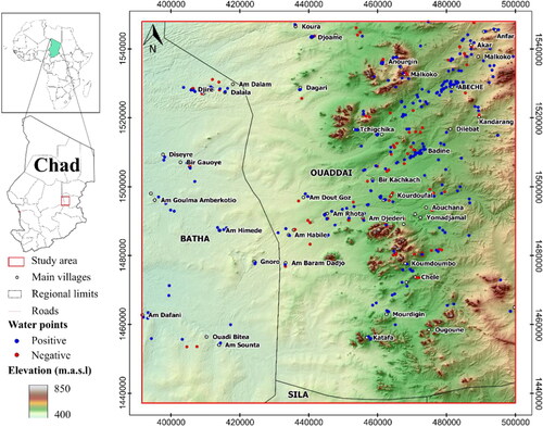
The landscape is predominantly flat towards the west (400 m.a.s.l.), and hillier towards the east, where altitudes exceed 850 m.a.s.l. Climate is hot semi-arid (BSh) as per the Köppen-Geiger classification. Mean daily temperature is 29 °C, ranging from 25 °C in January to 33 °C in May (Earthwise contributors 2017). Annual rainfall varies between 290 and 390 mm per year, distributed between the months of June and September-October. There is a certain irregular distribution of total precipitation between years. The effective rainfall, however, starts in June, as the low rainfall rates in May (generally < 10 mm/month) do not cause any significant change. Wadis start flowing between June and July, while small to medium-size rivers show surface runoff for a few weeks, the Batha river flows for about 3 months a year. In some particularly favourable years (i.e., 2019-2020) surface water accumulation can be observed up to November -December (MEH, in preparation). The region is characterized by a relatively dense river network, all of an ephemeral behaviour. Suitably, most of the region is sparsely vegetated and has seasonal patterns associated with the temporal distribution of rainfall. With the rains of June, the land covers progressively to whole vegetated. The peak is generally reached in august, then progressively decreases. Until December green areas are still visible, concentrating then only along the main wadi's course (i.e., Batha) from January on.

Close to 50% of the study area corresponds to open land without vegetation and 13% to cropland. Land uses such as dense vegetation, sparse vegetation, vegetation in rocky areas and humid open land appear to a lesser extent. A clear land cover gradient is observed from north to south. Desert landscapes predominate in the north, becoming a steppe or pseudo-steppe towards the central part. Shrubby savannah evolving into a wooded savannah and forest is observed further south (SSO, 2015). Arenosols take up 65% of the total surface area. These are best described as deep sandy soils, with high permeability. Vertisols (heavy clay soils with a high proportion of swelling clays), Cambisols (soils with at least an incipient subsurface soil formation) and Leptosols (very thin soils on continuous rock) are present in the 12%, 11% and 10% of the study area, respectively (IUSS Working Group WRB 2015)

Groundwater occurrence is heavily constrained by geological aspects (Figure 2). The study area is located along the borders of the Precambrian Massif of Ouaddaï, which conforms the eastern border of Lake Chad basin. Three major domains may be distinguished from the hydrogeological viewpoint (Upton et al. 2018). Crystalline rocks conform the central and eastern part. While these are impervious for practical purposes, fractures may store moderate amounts of groundwater. In the deeper valleys within the eastern granitic massifs, the crystalline substratum is weathered, thus resulting in low to moderate productivity aquifers. Piedmonts may also present a reasonable groundwater potential.

Figure 2. Main geological units of the study area.

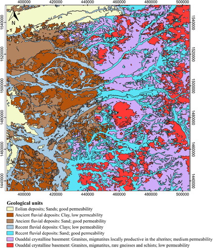
The Pliocene-Quaternary Chad formation predominates in the western part of the study area. The Chad formation consists mostly of unconsolidated sediments. While theoretically permeable, these are largely unproductive along the contact with crystalline outcrops. The transition zone between the crystalline basement and the productive sedimentary domain is known as the “biseau sec” (“dry fringe”). It represents an area where groundwater percolates from the crystalline outcrops into the sedimentary basin without necessarily resulting in a permanent water table (Figure 3).

Figure 3. Conceptual model of the "biseau sec" and principal hydrogeologic domains. Based on Detay et al. (1991).

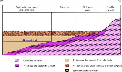
The third hydrogeological domain consists of Quaternary alluvium. Alluvium is associated with ephemeral streams running from the eastern highlands to the western flats. It is typically permeable and characterized by shallow water tables. Although of limited thickness and vulnerable to contamination, alluvial aquifers are important as a source of drinking water, as well as one of the most effective mechanism for the recharge of underlying crystalline and sedimentary units.

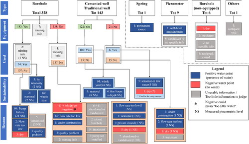
2.2. Borehole database and fieldwork verification

The national borehole database of Chad (SITEAU) comprises information on boreholes, springs, piezometers and dug wells (Figure 4). Prior to developing groundwater potential maps, all 488 water points were verified on a one-by-one basis during an extensive field campaign that took place between late 2019 and early 2020. Fieldwork focussed on validating coordinates, functional status and water point characteristics. The latter included use, equipment, seasonality, static level, electric conductivity and flow rate, among others. Outcomes were processed to determine the actual number of positive and negative water points in the region. The “positive” and “negative” labels are chiefly based on the presence of water at the moment of the inspection, as well as on reliability (seasonal vs. perennial). A water point was labelled positive when it provided enough water to supply a manual hand pump on a permanent basis. Those that operate seasonally but that were on use when inspected in the field were also considered positive. Conversely, negative points are those that failed to find groundwater during the drilling stage (or whose flow rate was < 0.5 m³/h). This classification led to 313 positive water points (74.7% of usable water points), 106 negative water points (25.3% of usable water points) and 69 water points that are unusable due to insufficient information. Additional negative training points were added to the dataset to represent both mountain outcrops and specific areas in the “biseau sec”. These are regions where borehole records are scarce, but where field experience confirms the absence of groundwater. This allowed to enrich the negative part of the dataset and reduce the imbalance between the positive and negative classes. All water points were subsequently incorporated into a QGIS 3 database.

Figure 4. Borehole database analysis. The location and status of all 488 water points in the study area was verified on site.

2.3. Mapping software and models

This research uses MLMapper 2.0, an evolution of the original MLMapper code developed by Martínez-Santos and Renard (2020). MLMapper provides spatially distributed predictions for a target variable based on supervised classification algorithms, a set of explanatory variables, and a training set of points where the outcome of the target variable is known (Figure 5). Major improvements to this update include automatic variable scaling, k-fold cross-validation procedures, feature number optimization and recursive feature elimination.

Figure 5. MLMapper methodological flowchart.

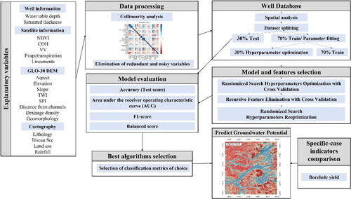
ML algorithms are inherently complex. Predicting whether one algorithm will outperform another, or whether an algorithm will yield good results on a given dataset, is typically unrealistic. To deal with this issue MLMapper applies a large number of ML classifiers from the SciKit-Learn 0.24.1 toolbox (Pedregosa et al. 2011). Then, it picks the best performers based on user-defined performance thresholds. MLMapper’s classifiers include support vector machines (SVC), linear support vector machines (LVC), logistic regression (LRG), decision tree classifier (CRT), random forest classifier (RFC), k-neighbor classification (KNN), linear discriminant analysis (LDA), Gaussian naïve Bayes classification (NBA), multilayer perceptron neural network (MLP), Ada-boost classifier (ABC), quadratic discriminant analysis (QDA), gradient boosting classification (GBC), Gaussian process classifier (GPC), ridge classifier (RID), stochastic gradient descent linear classifier (SGD), perceptron (PER), passive aggressive classifier (PASSI), nu-support vector classifier (nuSVC), and extra-trees classifier (ETC).

Several trial runs were carried out first, in order to identify the best performing algorithms. This led to the choice of random forest (RFC) and extra-tree (ETC) classifiers for the purpose of mapping groundwater potential.

RFC and ETC share a common background, as both use an ensemble application of the simple decision tree algorithm. RFC combines classifiers by averaging their probabilistic prediction (Breiman 2001). Each tree in the ensemble is built from a sample drawn with replacement (i.e., a bootstrap sample) from the training set. By splitting each node during the generation of a tree, the best split is found from all input features (explanatory variables) or from a random subset of the max_features parameter (the number of features to consider when looking for the best split). The aim of these two randomization sources is to decrease the variance of the forest estimator. Thus, RFC manages to reduce the variance compared to simple decision trees (high variance and tendency to overfit) by combining several trees, sometimes at the cost of a slight increase in bias. In practice, the reduction in variance is usually significant, resulting in an overall better model (Pedregosa et al. 2011).

ETC builds an ensemble of unpruned decision trees according to a classical top-down process (Geurts et al. 2006). Two major differences from other tree-based ensemble methods are that it splits the nodes by choosing the cut points completely randomly and that it uses the entire learning sample (instead of a bootstrap replica) to grow the trees.

2.4. Target variable and explanatory variables

In the case at hand, the target variable is groundwater potential, which is defined in binary terms as the likelihood that a borehole drilled at a given location would be positive.

Table 1 summarizes the explanatory variables used in this study. Figure 6 and Figure 7 show the maps of the most important explanatory variables according to the results obtained to predict GPM. Naghibi and Pourghasemi (2015) indicate that the importance of explanatory variables in GPM is considerably influenced by the characteristics of the study area. Díaz-Alcaide and Martínez-Santos (2019) identify the most frequent explanatory variables in groundwater potential studies. These include lithology, geological lineaments, landforms, topography, soil, land cover, drainage, slope-related variables, rainfall, and vegetation indices, among others. GPM assumes that the presence or absence of groundwater can be partially inferred from surface features. For instance, an inselberg is unlikely to hold groundwater, whereas the floodplain of a major river could be expected to be more productive. Similarly, a highly fissured area in crystalline outcrops is more likely to result in successful boreholes than areas where fracturing is absent. Subsoil information, such as borehole logs, is also important. The combination of stratigraphic columns and static levels can render estimates of saturated thickness, which also constrains borehole productivity.

Figure 6. Most important explanatory variables, according to the results obtained, used to predict GPM: (A) Aspect; (B) Basement depth; (C) COH Dry; (D) Evapotranspiration; (E) Fracture density 250 m radius; (F) Interpolated hydraulic heads from field measurements (January-February 2020); G) Rainfall; (H) Land use in the dry season; (I) Min COH difference.

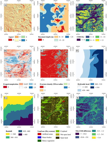
Figure 7. Most important explanatory variables, according to the results obtained, used to predict GPM: (A) NDVI Dry; (B) Slope; (C) Topographic wetness index; (D) Landforms; (E) Distance to ephemeral channels; (F) VV Dry.

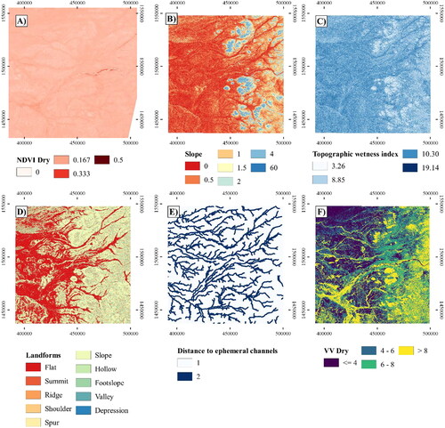
Table 1. Explanatory variable/shortname, description and information source.

Name/shorthand	Description	Unit of measurement	Source
COH Dry min	Minimum value of coherence dry season	Dimensionless	Sentinel-1
COH Wet min	Minimum value of coherence wet season	Dimensionless	Sentinel-1
Min COH difference	Difference between COH Dry min and COH Wet min	Dimensionless	Sentinel-1
VV Dry mean	Mean value of VV intensity dry season	dB	Sentinel-1
VV Wet mean	Mean value of VV intensity wet season	dB	Sentinel-1
Mean VV difference	Difference between VV Dry mean and VV Wet mean	dB	Sentinel-1
NDVI Dry	NDVI at end of the dry season (December 2017 - March 2018)	Dimensionless	Sentinel-2
NDVI Wet	NDVI at end of the wet season (June-September 2018)	Dimensionless	Sentinel-2
NDVI max	Maximum value of NDVI wet season	Dimensionless	Sentinel-2
Land cover dry	Land cover at end of the dry season (December 2017 - March 2018)	Dimensionless	Sentinel-1/-2
Land cover wet	Land cover at end of the wet season (June-September 2018)	Dimensionless	Sentinel-1/-2
Lithology	Geological domains per rock type	Dimensionless	Landsat-8
Precipitation	Cumulated precipitation wet season (June-September 2018)	Millimeter	MSG
Evapotranspiration	Evapotranspiration dry season (December 2017 - March 2018)	Millimeter per day	Landsat-8
Drainage density	Length of channels per unit area	km/km^2	AW3D-WorldDEM
Distance permanent channels	Distance to channels classified as permanent due to permanent seasonal regime	Dimensionless	AW3D-WorldDEM
1000 Fault	Fault density with a 1000 m radius	Dimensionless	AW3D-WorldDEM
2000 Fault	Fault density with a 2000 m radius	Dimensionless	AW3D-WorldDEM
Fracture density 100 m	Fracture density with a 100 m radius	Dimensionless	AW3D-WorldDEM
Fracture density 250 m	Fracture density with a 250 m radius	Dimensionless	AW3D-WorldDEM
Fracture density 50 m	Fracture density with a 50 m radius	Dimensionless	AW3D-WorldDEM
Distance ephemeral channels	Distance to channels classified as ephemeral due to their seasonal regime	Dimensionless	AW3D-WorldDEM
Geomorphology	Landform	Dimensionless	AW3D-WorldDEM
Stream Power Index	Describe potential flow erosion at the given point of the topographic surface	Dimensionless	AW3D-WorldDEM
Elevation	Topographic elevation	Meters above sea level (m.a.s.l.)	AW3D-WorldDEM
Aspect	Direction of the slope	Direction	AW3D-WorldDEM
Slope	Slope	Degree	AW3D-WorldDEM
Topographic wetness index	Steady state wetness index. Quantifies topographic control on surface hydrology.	Dimensionless	AW3D-WorldDEM
Saturated thickness	Difference between hydraulic heads and basement depth	Meters	Field data
Hydraulic head	Interpolated hydraulic heads from field measurements (January-February 2020)	Meters above sea level (m.a.s.l.)	Field data
Basement Depth	Interpolation of the stratigraphic data from borehole drilling	Meters	Field data

Satellite monitoring does not penetrate deep into the ground, but provides information about features that could be associated with the presence of groundwater (Díaz-Alcaide and Martínez-Santos 2019). This can be important in the case at hand, where the available data reveals that the static level is between 5-15 m below the surface in most cases. From Sentinel-1 time-series, VV- and VH-polarization intensity (backscattering coefficient) and VV- polarization coherence (interferometric correlation) are computed. The annual 12 days intensity and coherence data are split into dry (October-May) and wet (June-September) season, from which temporal descriptors, i.e., mathematical features – such as the absolute minimum and maximum, mean, mode, median, minimum and maximum gradient, etc. – describing the temporal signature (i.e., the seasonal variations) are derived (ESA n.d.; Holecz et al. 2015).

The same procedure applied to Sentinel-1 is exploited to Sentinel-2, in this case, temporal descriptors from Normalized Difference Vegetation Index (NDVI) time-series are derived. Vegetation-related indices can be useful in this context, particularly when computed at the end of the dry season. NDVI is an estimate of vegetation vigour and is derived from the response of vegetation to red and visible infrared wavelengths (Xie et al. 2008).

Sentinel-1 and Sentinel-2 time-series have been used to obtain a land cover map of the dry (Figure 6H) and wet seasons, respectively. Landsat-8 data during the dry season has been used to extract the lithology (Figure 2) by means of Sultan transformation (Sultan et al. 1987). Meteosat Second Generation (MSG) satellites and Tropical Applications of Meteorology using SATellite and ground-based observations (TAMSAT) were also used to obtain precipitation (Figure 6G) and evapotranspiration (Figure 6D).

Topography is a relevant factor in groundwater distribution, storage, and flow. It also controls surface runoff and infiltration, which are partially constrained by surface features and which can be parameterized from a digital elevation model (Elbeih 2015). A 30-meter DEM (AW3D-WorldDEM) has been generated by combining the ALOS World 3D 30m and the TanDEM-X 90m DEM. In this case, the DEM was used to develop the slope, slope aspect, topographic wetness index (TWI), stream power index (SPI) and geomorphology layers. The topographic wetness index (TWI) represents the ease with which water accumulates at the surface (Beven and Kirkby 1979), while the stream power index provides a measure of the erosive potential (Moore et al. 1991). The channel network is also obtained from the DEM, and used to elaborate a drainage density and stream distance maps.

Faults and fractures were identified by means of a geological interpretation of topographic indexes. Fractures (Figure 6E) are derived from an automatic extraction of lineaments (Akram et al. 2019; Ayman and Han 2019). Basement depth layer represents the interpolation of the stratigraphic data from borehole drilling. The depth of basement was defined as the depth of the non-weathered Precambrian crystalline rocks.

ML algorithms attempt to find associations between the explanatory variables and the likelihood of borehole success. Some authors show that it is advisable to pre-process the explanatory variables in order to avoid expert bias (Gómez-Escalonilla et al. 2021). Classifiers such as k-neighbours and support vector machines are affected by ranges because these algorithms rely on distances between data points to determine their similarity. Furthermore, algorithms using gradient descent optimization (logistic regression, neural networks), require data to be scaled because range differences lead to different step sizes in the gradient descent formula for each feature, which increases computational time.

Normalization of explanatory variables is carried out by aggregating classes, re-scaling nominal data, or a combination of both. This process adjusts the values of the explanatory variables (sometimes continuous variables) to certain intervals depending on the method chosen. The quartile method clusters the values of each variable into four intervals, ensuring that a similar number of samples are contained in each interval. Subsequently, each of these intervals is assigned an integer number. The MaxAbs scaler transforms the data to fall within the interval [-1, 1] by dividing by the largest maximum value for each variable. This work uses MaxAbs scaling to minimize operator bias. The SciKit-Learn 0.24.1 toolbox incorporates several built-in scaling methods, including standardization, maximal absolute scaler, maximal-minimal scaler and normalization (Pedregosa et al. 2011). Much like it occurs with the classifiers, MLMapper picks the best performing one and discards the others.

2.5. Performance metrics

Algorithm performance may be assessed as per several metrics. In this case, these include AUC curve, test scores and balanced score metrics. The AUC curve illustrates how the diagnostic ability of a binary classifier system varies with its discrimination threshold. In essence, it measures how well a given algorithm is able to distinguish between classes in a binary problem. Test score is conceptually simpler, as it represents the number of correct guesses over the total number of attempts on the test dataset. Finally, the balanced score metric is similar to test score, except that it accounts for class imbalances in the input dataset. By definition, the balanced score is the macro-average of recall scores per class or, equivalently, raw accuracy where each sample is weighted according to the inverse prevalence of its true class (Pedregosa et al. 2011).

2.6. Supervised classification method

Collinearity check takes place prior to training the algorithms. When two or more explanatory variables are highly correlated, it is advisable to remove at least one of them in order to avoid undue weight and/or unwanted noise. Collinearity may also hamper interpretability because the regression coefficients of certain algorithms are not uniquely determined (Martínez-Santos et al. 2021).

In the initial phase, the database was divided into 70% water points for training and 30% for validation (testing) of model performance. Algorithm training incorporates randomized-search parameter fitting. Randomized-search fitting is more flexible and computationally efficient than the grid-search parameter fitting routine built into MLMapper’s previous version. Randomized-search cross-validation optimizes a given metric, or set of metrics, and maximizes predictive accuracy by identifying the most suitable combination of parameters that govern each algorithm. In the present work, three metrics were used to optimize the algorithms: raw test score, AUC and balanced score. Cross-validated recursive feature elimination ensues. The goal is to quantify the importance that each algorithm attributes to each variable, as well as to eliminate those features that incorporate noise or detract from predictive accuracy. Noisy and redundant variables are recursively suppressed until the optimal number in reached (Pedregosa et al. 2011). Hyperparameters are finally re-optimized and the relative weight of explanatory variables is determined. The recursive elimination process is only available for those algorithms that use feature importance or coefficient weights.

A Partial Dependence Plot (PDP) were developed for all explanatory variables, including satellite-based products. PDPs show the marginal effect that one or two features have on the predicted outcome of a machine learning model (Friedman 2001). Once the models have been optimized and the most important variables have been selected, a performance threshold based on machine learning performance metrics is chosen to select those models that predict the target variable most effectively. Algorithms scoring above the threshold are considered for further analysis, while the others are discarded. Since each of the best-performing algorithms may rely on a different combination of explanatory variables, discrepancies among map outcomes are expected. An efficient way to observe these discrepancies is to develop a complete arithmetic-mean ensemble or a series of pairwise ensembles.

3. Results

3.1. Collinearity analysis

Figure 8 presents the results of the collinearity analysis. Pair wise correlation coefficients are expressed as a colour palette ranging from −1.0 in red (inverse correlation) to 1.0 in blue (direct correlation). There is no universal consensus as to what an acceptable correlation threshold is, although literature show examples of acceptable collinearity coefficients ranging between 0.40 and 0.85 (Dormann et al. 2013).

Figure 8. Pairwise correlation matrix for all explanatory variables.

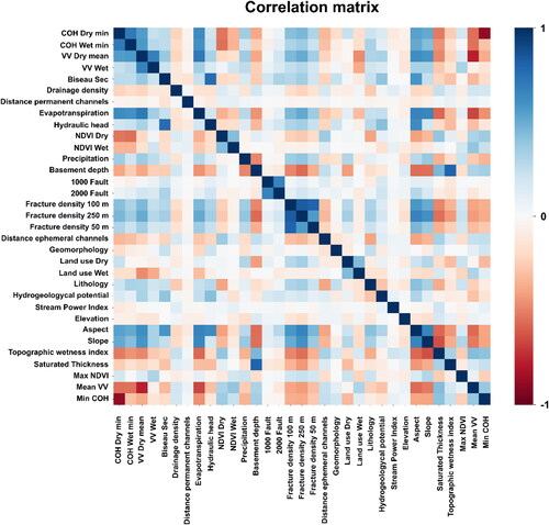
In this study, no strong direct correlations (>0.60) were observed. Negative correlations were found for “COH Dry min” versus “Min COH difference” and a positive correlation between “fracture density 100 m” versus “fracture density 250 m”. Both were expected to occur from the outset. In the first case, because the variable Min COH difference is obtained from the difference between the COH Min of the dry and wet seasons, a high correlation is to be expected. In the second case it stems from one variable being a spatial subset of the other. Due to the positive contribution of seasonal variables to the final score, no temporal variable was excluded for ensuing analyses.

3.2. Algorithm performance

Table 2 shows the evaluation metrics of the two best-performing algorithms, namely Extra Trees Classifier (ETC) and Random Forest Classifier (RFC). Metrics are shown for each algorithm, as well as for the random search and cross-validated recursive feature elimination processes. Test scores exceeded 0.80, area under the curve exceeded 0.87, and the balanced score metric exceeded 0.79 in all cases. A higher f-1 score is observed for the positive outcome (over 0.84), which is the most common one in the input database. However, the f-1 score of the negative class exceeds 0.78 in most cases (0.81 at best). This indicates that the algorithms are capable of distinguishing positive and negative classes accurately. The AUC ranging from 0.87 to 0.90 implies that the best-performing algorithms have a high probability of adequately predicting the target variable.

Table 2. Performance scores of the RFC and ETC classifiers. (Train = optimized training score; Test = optimized test score; Prec_0 = precision false; Prec_1 = precision true; Rec_0 = recall false; Rec_1 = recall true; f1_0 = f-1 score false; f1_1 = f-1 score true; AUC = area under curve).

Classifier	Train	Test	Prec 0	Prec 1	Rec 0	Rec 1	f1 score 0	f1 Score 1	AUC	Balanced score
Test score metric optimization
RFC	0.88	0.84	0.94	0.78	0.70	0.96	0.81	0.86	0.87	0.83
ETC	0.98	0.84	0.93	0.79	0.72	0.95	0.81	0.86	0.88	0.84
AUC metric optimization
RFC	0.94	0.82	0.90	0.78	0.70	0.93	0.79	0.85	0.88	0.82
ETC	0.82	0.80	1.00	0.72	0.58	1.00	0.73	0.84	0.88	0.79
Balanced score metric optimization
RFC	0.86	0.83	0.95	0.77	0.68	0.97	0.79	0.86	0.88	0.83
ETC	0.91	0.82	0.95	0.76	0.66	0.97	0.78	0.85	0.90	0.81

Optimizing test score rendered 0.84 for both algorithms, while also maximizing balanced score (0.83 and 0.84 for RFC and ETC, respectively). The highest AUC value was obtained by using the balanced score as metric optimization (0.88 and 0.90 for RFC and ETC, respectively). In contrast, the test score and the balanced score decrease when the AUC metric is selected as optimization metrics. Hyperparameter optimization by random search procedure led to the scores in Table 3.

Table 3. Algorithm hyperparameters (description after Pedregosa et al. 2011) and adjusted outcomes. Max_depth = The maximum depth of the tree; max_features = The number of features to consider when looking for the best split; min_samples_leaf = The minimum number of samples required to be at a leaf node; n_estimators = Number of trees in the ensemble methods; random_state = Controls both the randomness of the bootstrapping of the samples used when building trees and the sampling of the features to consider when looking for the best split at each node.

Classifier	Hyperparameter	Best Parameters
		Test score optimization	AUC optimization	Balanced score optimization
RFC	max_depth	5	9	9
	max_features	Sqrt	sqrt	log2
	min_samples_leaf	4	4	14
	n_estimators	306	346	156
	random_state	0	0	0
ETC	max_depth	8	5	8
	max_features	0.9	sqrt	0.8
	min_samples_leaf	1	3	4
	n_estimators	860	860	650
	random_state	0	0	0

3.3. Explanatory variable selection and importance

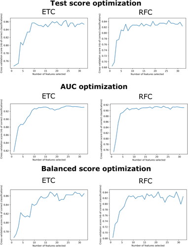
Recursive feature elimination identified different optimal patterns of explanatory variables, depending on the algorithm of choice and the optimization metric selected. Figure 9 shows the number of selected features versus the cross-validation score. This uses a 10-fold cross-validation to evaluate which variables are important. However, the algorithms internally discard those variables that allow to optimize the metric of choice. Thus, ETC used 24 explanatory variables to maximize test score, 25 when the AUC were used as optimization metric and 17 for balanced score. RFC used 26, 23, and 21 explanatory variables for the test score, AUC and balanced score, respectively.

Figure 9. Results of feature number optimization analysis for ExtraTrees and Random Forest using the test score, AUC and balanced score as optimization metrics.

Figure 10 shows the feature importance for both algorithms under each of the optimization procedures. ETC attributes a high importance to the “fracture density 250 m” layer (0.11, 0.12 and 0.13 for the test score, AUC and balanced score optimization procedures, respectively). “COH dry”, “slope”, “topographic wetness index”, “basement depth” and “distance to ephemeral channels” were also considered important conditioning factors. For the RFC algorithm, “slope”, “topographic moisture index”, “basement depth” and “aspect” were the most important explanatory variables. The combined importance of these four factors is 0.45, 0.39 and 0.51 for the test score, AUC and balanced score metrics, respectively.

Figure 10. Feature importance calculated for the best performing tree-based algorithms using the test score, AUC and balanced score as optimization metrics. The sum of all variable weights equals one.

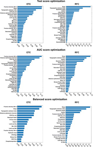
Eleven explanatory variables were found to be important in all cases. These were “aspect”, “basement depth”, “COH dry”, “evapotranspiration”, “fracture density 250 m”, “hydraulic heads”, “lithology”, “NDVI dry”, “slope”, “topographic wetness index” and “VV dry”. Seven conditioning factors were used in five cases: “COH wet”, “land cover dry”, “land cover wet”, “min COH”, “precipitation”, “saturated thickness” and “VV wet”. In contrast, “2000 Fault”, “distance to permanent channels” and “fracture density 50 m” were not used in any case. “Topographic elevation”, “geomorphology” and “1000 Fault” were used in three cases, while the “Max NDVI” was only relied upon once.

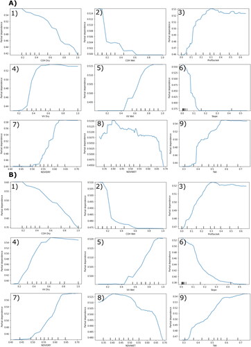
Figure 11 shows the PDP outcomes for RFC and ETC when test score is used as the optimization metric. The X-axis represents the values of the explanatory variables. These range from 0 to 1 due to the preprocessing approach. Higher values on the Y-axis represent greater probabilities of positive groundwater potential. Outcomes are consistent with the hydrogeological context, with lower values of COH for dry and wet season, NDVI for wet season and slope leading to positive groundwater potential. Conversely, higher values of VV (dry and wet season), NDVI for dry season, basement depth and TWI lead to positive groundwater potential.

Figure 11. Partial Dependence Plot calculated for the most important variables and for explanatory variables derived from seasonal fluctuations of satellite-based products when using the test score as optimization metrics. A) PDP of RFC; B) PDP of ETC; (1) COH dry; (2) COH wet; (3) Basement depth; (4) VV dry; (5) VV wet; (6) Slope; (7) NDVI dry; (8) NDVI wet; (9) TWI.

3.4. Groundwater potential maps

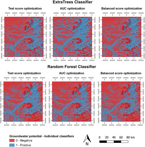
Classifier outcomes were extrapolated to produce groundwater potential maps. Figure 12 shows the groundwater potential predictions rendered by each algorithm under the three different metrics used as the optimization objective. Blue areas are those in which the algorithms found a combination of explanatory variables leading to a positive potential, while red zones represent a negative groundwater potential. ETC predicted a positive groundwater potential for the 43% of the surface area when using test score and balanced score as optimization metrics. The extent of positive potential prediction increases to 53% when the AUC metric is used. RFC predicts a larger area for the negative potential class in all cases (56%, 61% and 61% for the test score, AUC and balanced score optimization procedures, respectively).

Figure 12. Mapping outcomes of the extra trees and random forest classifiers for the three optimization metrics (test score, AUC and balanced score).

Figure 13 shows the outcomes of the ensemble map for test score, AUC and balanced score as optimization metrics. This map allows for an analysis of discrepancies between both algorithms. Pixel scores are computed as the simple arithmetic mean between the ETC and RFC outcomes. Blue pixels mean that both algorithms agreed on a positive groundwater potential (arithmetic mean = 1). Conversely, red zones represent those pixels where both algorithms agreed on a negative groundwater potential (0). Yellow represents disagreement between RFC and ETC outcomes (0.5).

Figure 13. Agreement map for test score (A), AUC (B) and balanced score (C) as optimization metrics. (D) Spatial distribution of negative boreholes and positive boreholes with known flow rates.

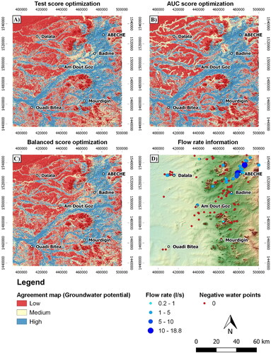
Table 4 presents these results in terms of surface area. All cases agree that around 45% of the total surface area corresponds to a negative groundwater potential. The agreement map obtained with the AUC score as an optimization metric showed the highest area of positive potential (34.7%) in comparison to the map obtained with test score (32.9%) and balanced score (28.7%).

Table 4. Quantification of the area corresponding to each class in the agreement map for test score, AUC and balanced score as optimization metrics.

Agreement Test Score
Value	Area (km^2)	Area (%)
0	5467.83	45.65
0.5	2571.26	21.47
1	3937.81	32.88
Agreement AUC Score
Value	Area (km^2)	Area (%)
0	5148.96	43.08
0.5	2656.33	22.23
1	4145.48	34.69
Agreement Balanced Score
Value	Area (km^2)	Area (%)
0	5686.08	47.48
0.5	2853.69	23.82
1	3437.13	28.70

4. Discussion

4.1. Model selection and feature importance

RFC and ETC were observed to consistently outperform all other algorithm families in MLMapper, including logistic regression, discriminant analyses and support vector machines. This confirms the results obtained in previous studies (Martínez‐Santos and Renard 2020; Arabameri et al. 2021; Gómez-Escalonilla et al., in press) as well as the advantages of combining simple tree predictors (Breiman 2001).

The choice of algorithms and explanatory variables is constrained by different factors. The most important one is that groundwater potential has a different meaning to the different researchers (Díaz-Alcaide and Martínez-Santos 2019). This implies that explanatory variables will differ depending on whether we attempt to predict, for instance, borehole yield or spring occurrence. Therefore, the results of our work must be placed in the context of equivalent undertakings. Naghibi, Moghaddam, et al. (2017) used a series of supervised classification techniques to map well potential mapping in the Kashmar region of Iran. These authors identified a bagging algorithm as the best performer, and different combinations of NDVI, slope, altitude, distance from rivers and land cover as the best predictors for groundwater potential. Along the same lines, Lee et al. (2020) mapped groundwater yield potential in Yangpyeong-Gun, South Korea, by means of a combination of probabilistic models and a boosted classification tree algorithm. Soil, topographic texture, forest type and land cover were identified as the single most important conditioning factors, whereas valley depth and topographic position index ranked among the least important. Miraki et al. (2019) worked with a combination of RFC, logistic regression and naïve Bayes classifiers, concluding that topographic wetness index, drainage density and slope-related factors were more important than fault density, stream power index and land cover. In the case at hand, fracture density, slope, SAR coherence, TWI, basement depth, distance to ephemeral channels and slope aspect proved the most important variables. A necessary corollary to all this is that both the algorithms and conditioning factors of choice are case-specific. Therefore, working with an ample range of explanatory variables and machine learning algorithms is an appropriate course of action in GPM studies. We also observe that the choice of scoring metrics can attribute different weights to explanatory variables. In turn, this may result in a different set of key predictors for groundwater occurrence.

In our view, an important contribution of this research is the use of seasonal variables, which are seldom represented in ML GPM studies (Díaz-Alcaide and Martínez-Santos 2019). Outcomes reveal that dry season products are particularly significant. This is attributed to the greater contrast that the dry season offers in relation to groundwater. Take for instance vegetation vigour. During the dry season temperatures are high and rainfall is practically absent. Therefore, patches of vigorous vegetation may reflect the nearby presence of permanent surface water, irrigation, and/or a shallow water table. On the other hand, the wet season is characterized by large expanses of land with a high moisture content. This leads to a less clear signal as to whether shallow groundwater is the cause behind a vigorous vegetation.

PDP results facilitate the interpretation of the model outcomes (Figure 11). Flat areas (low slope values) have a positive impact on groundwater potential. This is consistent with the conceptual model of aquifer recharge, in which the flatter sectors allow water infiltration into the aquifer layers. Higher TWI values represent areas where flow accumulation results in a higher moisture index, so infiltration or exfiltration rates are expected to be higher. The partial dependence on basement depth shows the expected results, a greater basement depth could represent a thicker weathered zone (i.e., thicker porous aquifer conditions therefore higher storage capacity). From a hydrogeological point of view, the productivity of those areas is higher than that of the sectors where unweathered crystalline basement outcrop at the surface or with a shallow weathered zone.

The COH for the dry and wet seasons have similar relation with GPM, but the COH for wet season presents a clearer PDP trend. VV values for the dry season are strongly discriminative in terms of GPM, as higher VV values lead to a positive GPM in both, dry and wet season. The reasoning applies to the VV for the wet season, but the values required to obtain a positive GPM must be higher than in the dry season. Finally, the NDVI of the dry and wet seasons shows very different trends. Higher values of NDVI for the dry season led to a positive GPM, which is in agreement with previous studies carried out by Mandal et al. (2016) and Kamali Maskooni et al. (2020). Lower values of NDVI for the wet season led to a positive GPM which is also consistent with the literature (Nampak et al. 2014).

4.2. Groundwater potential maps in the context of regional hydrogeological conditions and limitations of the outcomes

Figure 13 presents the degree of agreement between the RFC and ETC algorithms. RFC and ETC maps resemble each other to a large extent, differences pertaining mostly to fringe areas around outcrops, as well as to small valleys. All maps present a high correlation with geological and hydrogeological elements (see also Figure 6 and Figure 7). High potential is predominantly associated with valleys carved out by ephemeral streams. Weathered crystalline materials and piedmonts also result in suitable areas for groundwater development. Low potential occurs within basement outcrops in the east. The presence of low groundwater potential areas in the west is also consistent with the conceptual description of a “biseau sec” (dry fringe) provided by Detay et al. (1991).

Martínez-Santos et al. (2021) contend that ML results should be verified with independent indicators whenever possible. In this case, extensive fieldwork rendered a limited number of boreholes and wells (n = 34) for which flowrate data could be obtained. Flow rates are meaningful in as much as these provide ground truth on aquifer productivity. In other words, a valid groundwater potential map would be expected to highlight in blue those areas where the highest flow rates exist, and should represent in red those areas where most boreholes are either seasonal or negative. Nevertheless, flow rate data presents shortcomings of its own. For instance, a negative borehole drilled in a theoretically favourable area may be the result of poor construction, of not reaching deep enough, and/or of not providing as much water as required, rather than the consequence of groundwater being actually absent. Furthermore, in an area where hand pumps are common, flowrates around 1 m³/h are questionable, as this value could reflect the capacity of the hand pump, rather than that of the borehole itself. Therefore, interpretations based on comparing flowrates with maps are partially qualitative.

Figure 13D depicts a reasonable agreement between ML outcomes and borehole yields. Wadis and piedmonts are identified as the most productive areas, which is consistent with hydrogeological knowledge for crystalline domains such as the one at hand. The highest yields were located near Abeché, in the northeastern part of the study area. This zone presents a combination of the wadis and a thicker zone of weathered crystalline basement rocks, thus showing the greater potential for groundwater development. While this is consistent with field experience, it is also known that borehole yields currently struggle to meet the needs of the population. In other words, high groundwater potential should be interpreted as an area where groundwater is more likely to be found, but further work needs to be conducted to predict yield. Other wells with major flow rates located in the Badine, Dalala and Am Dout Goz were also adequately identified on the agreement maps. The latter are located in the wadis of the western region. In addition, the negative points located west of the Badine, south of Am Dout Goz and Ouadi Bitea and around Dalala were also correctly identified by the ML approach.

Precedents of groundwater potential maps in the study area are scarce and based on expert knowledge. Al-Djazouli et al. (2019 and 2021) relied on principal component analysis and satellite images to map fracture systems in the Ouaddaï region, and subsequently developed estimates of groundwater potential based on an expert-based analytical hierarchical procedure. Differences in terms of scale, method and geographical extent make their outcomes difficult to compare with ours. Hence, our approach and results should be interpreted as a complementary overview that zooms into the border of the Ouaddaï and Batha regions.

In addition, an expert-based groundwater potential map of the study area was previously developed by some of the co-authors of this paper (MEH, in preparation). They identified alluvial sediments and weathered crystalline materials as the most suitable for groundwater development, while basement outcrops, argillaceous materials, and aeolian sands as the least likely to hold groundwater. Similar findings in this research attests the potential of automated approaches for the identification of regions of good groundwater prospect, even though binary classification is only partially informative in terms of aquifer productivity. Methodological inroads should be made towards a finer classification of groundwater potential. The main limitations of this study relate to the number of points available for the training/testing process. Machine learning approaches are based on the assumption of big data methods, where a large number of samples is usually required for the algorithms to find meaningful associations, and hence, better predictions. Conducting pumping tests at all wells and extending the study region to enhance the database would likely contribute to this goal.

Additionally, the high-medium-low classification is somewhat loose. Inroads should be made in the future towards predicting actual borehole yield based on improved field data. This entails working with detailed information such as transmissivity, specific flow rates and/or storage coefficients, which is typically difficult to come by in national and regional-scale databases. Incorporating water quality would also contribute to more meaningful results in terms of water resources planning and management.

5. Conclusions

Groundwater is a crucial resource in arid regions of developing countries, where a large share of the population relies on boreholes and excavated wells for drinking supply. Groundwater potential mapping is increasingly relied upon in these geographical contexts due to the difficulties involved in large-scale groundwater exploration. This paper has presented a ML approach to develop GPM, and has illustrated it through its application to the Ouaddaï and Batha regions, eastern Chad.

From a methodological standpoint, this research highlights the advantages of using a large number of supervised classification methods in order to quickly identify the best performers and discard those that render worse results. In the present case, ensemble tree-based algorithms have proven to be the most efficient. Optimizing algorithm hyperparameters to maximize different metrics rendered roughly equivalent outcomes in terms of spatial predictions, but also resulted in a different choice of conditioning factors. This suggests that this kind of analysis should be carried out routinely in groundwater potential studies, particularly if spatial predictions happen to differ significantly from one performance metric to another. In addition, it is advisable to take into account seasonal fluctuations of satellite-based explanatory variables. While COH, VV and NDVI have different responses and importance in predicting GPM, the benefits of using these variables in GPM research cannot be overlooked.

From a case-specific perspective, the results show the areas of best groundwater prospect to take place in valleys and piedmonts. Areas where the depth to basement is greater also correlate with higher groundwater potential. Conversely, basement outcrops and the transition zone between the crystalline mountains, to the east, and the sedimentary basin, to the west, are less likely to result in productive boreholes. These findings are conceptually in agreement with the hydrogeological contexts such as the one at hand, and consistent with the available flow rate data.

Finally, this method is based on an open-source piece of software that is versatile enough to incorporate any choice of explanatory variables. This means that the technique can be readily exported to any geographical setting for which spatially-distributed predictors of groundwater occurrence may be developed. An improved database with information derived from pumping tests and the incorporation of more water points would provide better predictions for future studies.

Acknowledgements

This research was carried out under the ResEau project, co-funded by the Government of Chad and the Swiss Agency for Development and Cooperation (SDC). MLMapper was updated under grant RTI2018-099394-B-I00 of Spain’s Ministerio de Ciencia, Innovación y Universidades. The first author received an FPI grant from the Ministerio de Ciencia e Innovación to develop his PhD within this project (PRE2019-090026).

Disclosure statement

The authors declare that they have no known competing financial interests or personal relationships that could have appeared to influence the work reported in this paper.

Data not available due to legal restrictions

References

- Akram MS, Mirza K, Zeeshan M, Ali I. 2019. Correlation of Tectonics with Geologic Lineaments Interpreted from Remote Sensing Data for Kandiah Valley, Khyber-Pakhtunkhwa, Pakistan. J Geol Soc India. 93(5):607–613.
- Al-Djazouli, MO, Elmorabiti K, Rahimi A, Amellah O, Fadil OAM. 2021. Delineating of groundwater potential zones based on remote sensing, GIS and analytical hierarchical process: a case of Waddai, eastern Chad. GeoJournal. 86(4):1881–1894.
- Al-Djazouli MO, Elmorabiti K, Zoheir B, Rahimi A, Amellah O. 2019. Use of Landsat-8 OLI data for delineating fracture systems in subsoil regions: implications for groundwater prospection in the Waddai area, eastern Chad. Arab J Geosci. 12(7):241. DOI 10.1007/s12517-019-4354-8
- Arabameri A, Pal SC, Rezaie F, Nalivan OA, Chowdhuri I, Saha A, Lee S, Moayedi H. 2021. Modeling groundwater potential using novel GIS-based machine-learning ensemble techniques, J Hydrol Reg Stud. 36:100848.
- Ayman S, Han L. 2019. Effects of vertical accuracy of digital elevation model (DEM) data on automatic lineaments extraction from shaded DEM. Adv Space Res. 64(3):603–622.
- Beven KJ, Kirkby MJ. 1979. A physically based, variable contributing area model of basin hydrology/Un modèle à base physique de zone d’appel variable de l’hydrologie du bassin versant, Hydrol Sci Bull. 24(1):43–69.
- Breiman L. 2001. Random Forests. Mach Learn. 45(1):5–32.
- Chen Y, Chen W, Chandra Pal S, Saha A, Chowdhuri I, Adeli B, Janizadeh S, Dineva AA, Wang X, Mosavi A. 2021. Evaluation efficiency of hybrid deep learning algorithms with neural network decision tree and boosting methods for predicting groundwater potential. Geocarto Int. 1–21.
- Chen W, Li Y, Tsangaratos P, Shahabi H, Ilia I, Xue W, Bian H. 2020. Groundwater spring potential mapping using artificial intelligence approach based on kernel logistic regression, random forest, and alternating decision tree models. Appl. Sci. 10(2):425.
- Chen W, Zhao X, Tsangaratos P, Shahabi H, Ilia I, Xue W, Wang X, Ahmad BB. 2020. Evaluating the usage of tree-based ensemble methods in groundwater spring potential mapping. J. Hydrol. 583:124602.
- Detay M, Poyet P, Castany G, Bernardi A, Casanova R, Emsellem Y, Brisson E, Aubrac G. 1991. Hydrogéologie de la limite Sud-Ouest du bassin du Lac Tchad au Nord Cameroun - mise en évidence d’un aquifère semi-captif de socle dans les zones de piémont et de « biseau sec ». Comptes Rendus Geosci. 312:1049–1056.
- Díaz-Alcaide S, Martínez-Santos P. 2019. Review: Advances in groundwater potential mapping. Hydrogeol J. 27(7):2307–2324
- Díaz-Alcaide S, Martínez-Santos P, Villarroya F. 2017. A commune-level groundwater potential map for the Republic of Mali. Water. 9(11):839.
- Dormann CF, Elith J, Bacher S, Buchmann C, Carl G, Carré G, Marquéz JRG, Gruber B, Lafourcade B, Leitão PJ, Münkemüller T. 2013. Collinearity: a review of methods to deal with it and a simulation study evaluating their performance. Ecography. 36(1):27–46.
- Earthwise contributors. 2017. Climate of Chad. Accessed: 15 June 2021. http://earthwise.bgs.ac.uk/index.php?title=Climate_of_Chad&oldid=32806
- Elbeih SF. 2015. An overview of integrated remote sensing and GIS for groundwater mapping in Egypt. Ain Shams Engineering Journal 6(1):1–15.
- European Space Agency (ESA). n.d. Sentinel-1 SAR user guide. https://sentinel.esa.int/web/sentinel/user-guides/sentinel-1-sar
- Fadhillah MF, Lee S, Lee CW, Park YC. 2021. Application of support vector regression and metaheuristic optimization algorithms for groundwater potential mapping in Gangneung-si, South Korea. Remote Sensing. 13(6):1196.
- Forootan E, Seyedi F. 2021. GIS-based multi-criteria decision making and entropy approaches for groundwater potential zones delineation. Earth Sci Inform. 14(1):333–347.
- Friedman JH. 2001. Greedy function approximation: a gradient boosting machine. Annals of statistics, 29(5):1189–1232.
- Geurts P, Ernst D, Wehenkel L. 2006. Extremely randomized trees. Mach Learn. 63(1):3–42.
- Gómez-Escalonilla V, Martínez-Santos P, Martín-Loeches M. 2021. Preprocessing approaches in machine learning-based groundwater potential mapping: an application to the Koulikoro and Bamako regions, Mali, Hydrol. Earth Syst Sci Discuss., in review.
- Grönwall J, Danert K. 2020. Regarding groundwater and drinking water access through a human rights lens: self-supply as a norm. Water. 12(2), 419.
- Ha DH, Nguyen PT, Costache R, Al-Ansari N, Van Phong T, Nguyen HD, Amiri M, Sharma R, Prakash I, Van Le H, Nguyen HBT. 2021. Quadratic discriminant analysis based ensemble machine learning models for groundwater potential modeling and mapping. Water Resour Manag. 35(13):4415–4433.
- Harvey P. 2004. Borehole sustainability in Rural Africa: An analysis of routine field data. 30th WEDC International Conference. Vietiane, Lao PDR.
- Holecz F, Gatti L, Collivignarelli F, Barbieri M. 2015. On the use of temporal-spectral descriptors for crop mapping, monitoring and crop practices characterization, IGARSS Symposium, Milan.
- IUSS Working Group WRB. 2015. World Reference Base for Soil Resources 2014. Rome: FAO.
- Jha MK, Chowdhury A, Chowdary VM, Peiffer S. 2007. Groundwater management and development by integrated remote sensing and geographic information systems: prospects and constraints. Water Resour Manag. 21(2):427–467.
- Kamali Maskooni E, Naghibi SA, Hashemi H, Berndtsson R. 2020. Application of advanced machine learning algorithms to assess groundwater potential using remote sensing-derived data. Remote Sens. 12(17):2742.
- Lee S, Hyun Y, Lee S, Lee MJ. 2020. Groundwater Potential Mapping Using Remote Sensing and GIS-Based Machine Learning Techniques. Remote Sens. 12(7):1200.
- MacDonald AM, Bonsor HC, Dochartaigh BÉÓ, Taylor RG. 2012. Quantitative maps of groundwater resources in Africa.Environ. Res. Lett. 7(2):024009.
- Mandal U, Sahoo S, Munusamy SB, Dhar A, Panda SN, Kar A, Mishra PK. 2016. Delineation of groundwater potential zones of coastal groundwater basin using multi-criteria decision making technique.Water Resour Manag. 30(12):4293–4310.
- Martínez-Santos P, Renard P. 2020. Mapping Groundwater Potential Through an Ensemble of Big Data Methods. Ground Water 58(4):583–597.
- Martínez-Santos P, Aristizábal HF, Díaz-Alcaide S, Gómez-Escalonilla V. 2021. Predictive mapping of aquatic ecosystems by means of support vector machines and random forests. Journal of Hydrol. 595:126026.
- MEH. In preparation. Carte hydrogéologique de la République du Tchad au 1:200,000. Ouvrages et Ressources. Feuille ND 34-09 Abéché. Pré-tirage réalisé par UNITAR et Swisstopo. Genève et Wabern, Switzerland.
- Miraki S, Zanganeh SH, Chapi K, Singh VP., Shirzadi A, Shahabi H, Pham BT. 2019. Mapping groundwater potential using a novel hybrid intelligence approach. Water Resour Manag. 33(1):281–302.
- Mohammadi-Behzad HR, Charchi A, Kalantari N, Nejad AM, Vardanjani HK. 2019. Delineation of groundwater potential zones using remote sensing (RS), geographical information system (GIS) and analytic hierarchy process (AHP) techniques: a case study in the Leylia–Keynow watershed, southwest of Iran. Carbonates Evaporites. 34(4):1307–1319.
- Moore ID, Grayson RB, Ladson AR. 1991. Digital terrain modelling: A review of hydrological, geomorphological, and biological applications, Hydrol Process. 5(1):3–30.
- Mosavi A, Sajedi Hosseini F, Choubin B, Goodarzi M, Dineva AA, Rafiei Sardooi E. 2021. Ensemble Boosting and Bagging Based Machine Learning Models for Groundwater Potential Prediction. Water Resour Manag. 35(1):23–37.
- Muchingami I, Chuma C, Gumbo M, Hlatywayo D, Mashingaidze R. 2019. Review: Approaches to groundwater exploration and resource evaluation in the crystalline basement aquifers of Zimbabwe. Hydrogeol J. 27(3):915–928.
- Naghibi SA, Ahmadi K, Daneshi A. 2017. Application of Support Vector Machine, Random Forest, and Genetic Algorithm Optimized Random Forest Models in Groundwater Potential Mapping. Water Resour Manage. 31(9):2761–2775.
- Naghibi SA, Moghaddam DD, Kalantar B, Pradhan B, Kisi O. 2017. A comparative assessment of GIS-based data mining models and a novel ensemble model in groundwater well potential mapping. Journal of Hydrology 548:471–483.
- Naghibi SA, Pourghasemi HR. 2015. A Comparative Assessment Between Three Machine Learning Models and Their Performance Comparison by Bivariate and Multivariate Statistical Methods in Groundwater Potential Mapping. Water Resour Manag. 29(14):5217–5236.
- Naghibi SA, Pourghasemi HR, Abbaspour K. 2018. A comparison between ten advanced and soft computing models for groundwater qanat potential assessment in Iran using R and GIS. Theor Appl Climatol. 131(3-4):967–984.
- Nampak H, Pradhan B, Abd Manap M. 2014. Application of GIS based data driven evidential belief function model to predict groundwater potential zonation. Journal of Hydrology, 513:283–300.
- Nguyen PT, Ha DH, Jaafari A, Nguyen HD, Van Phong T, Al-Ansari N, Prakash I, Le HV, Pham BT. 2020. Groundwater Potential Mapping Combining Artificial Neural Network and Real AdaBoost Ensemble Technique: The DakNong Province Case-study, Vietnam. IJERPH. 17(7):2473.
- Oursingbé M, Tang Z. 2011. Study of hydrogeological potential in the basement areas in eastern Chad: a case study of Ouaddaï-Biltine. Researcher. 3(2):91–100.
- Panahi M, Sadhasivam N, Pourghasemi HR, Rezaie F, Lee S. 2020. Spatial prediction of groundwater potential mapping based on convolutional neural network (CNN) and support vector regression (SVR). Journal of Hydrology 588:125033. doi.org/10.1016/j.jhydrol.2020.125033
- Park S, Kim J. 2021. The predictive capability of a novel ensemble tree-based algorithm for assessing groundwater potential. Sustainability. 13(5):2459.
- Pedregosa F, Varoquaux, G, Gramfort A, Michel V, Thirion B, Grisel O, Blondel M, Prettenhofer P, Weiss R, Dubourg V, et al. 2011. Scikit-learn: Machine learning in Python. Mach Learn Python. 12:2825–2830.
- Phong TV, Pham BT, Trinh PT, Ly H‐B, Vu QH, Ho LS, Le HV, Phong LH, Avand M, Prakash I. (2021). Groundwater potential mapping using GIS‐based hybrid artificial intelligence methods. Groundwater, 5, 745, 760, 59.
- Pradhan AMS, Kim YT, Shrestha S, Huynh T-C, Nguyen BP. 2021. Application of deep neural network to capture groundwater potential zone in mountainous terrain, Nepal Himalaya. Environ Sci Pollut Res Int. 28(15):18501–18517.
- Rahmati O, Avand M, Yariyan P, Tiefenbacher JP, Azareh A, Bui DT. 2021. Assessment of Gini-, entropy- and ratio-based classification trees for groundwater potential modelling and prediction. Geocarto Int. 15:1–20.
- Sachdeva S, Kumar B. 2021. Comparison of gradient boosted decision trees and random forest for groundwater potential mapping in Dholpur (Rajasthan), India. Stoch Environ Res Risk Assess. 35(2):287–306.
- Schetselaar EM, Harris JR, Lynds T, de Kemp EA. 2007. Remote predictive mapping 1. Remote Predictive Mapping (RPM): A strategy for geological mapping of Canada’s North. GS 34(3):93–111. https://journals.lib.unb.ca/index.php/GC/article/view/10248
- Sultan M, Arvidson RE, Sturchio NC, Guinness EA. 1987. Lithologic mapping in arid regions with Landsat thematic mapper data: Meatiq dome, Geol Soc Am Bull. 99(6):748–762. DOI 10.1130/0016-7606(1987)99 < 748:LMIARW>2.0.CO;2
- Tamiru H, Wagari M. 2021. Comparison of ANN model and GIS tools for delineation of groundwater potential zones, Fincha Catchment, Abay Basin, Ethiopia, Geocarto Int. 1–19.
- Tolche AD. 2021. Groundwater potential mapping using geospatial techniques: a case study of Dhungeta-Ramis sub-basin, Ethiopia. Geol Ecol Landscapes 5(1):65–80.
- UNESCO. 2015. editor. The United Nations World Water Development Report 2015: Water for a sustainable world. Paris, France: UNESCO.
- Upton K, Ó Dochartaigh BÉ, Bellwood-Howard I. 2018. Africa groundwater atlas: hydrogeology of Chad. British Geological Survey. Accessed June 2021. http://earthwise.bgs.ac.uk/index.php/Hydrogeology_of_Chad
- Verjee F, Gachet A. 2007. Mapping water potential: the use of WATEX to support UNHCR refugee camp operations in Eastern Chad. Perspect Soc Vulnerability. 94:1–16.
- Xie Y, Sha Z, Yu M. 2008. Remote sensing imagery in vegetation mapping: a review, J Plant Ecol. 1 (1):9–23.
- Yen HPH, Pham BT, Van Phong T, Ha DH, Costache R, Van Le H, Nguyen HD, Amiri M, Van Tao N, Prakash I. 2021. Locally weighted learning based hybrid intelligence models for groundwater potential mapping and modeling: A case study at Gia Lai province, Vietnam. Geoscience Frontiers. 12(5):101154.