Developing a high-resolution land use/land cover map by upgrading CORINE’s agricultural components using detailed national and pan-European datasets

Abstract

The agricultural uses of the Coordination of Information on the Environment Land Cover (CLC) dataset suffer from limitations such as temporal stationarity, low spatial resolution, broad and rather simplified grouping of classes. The study attempts to address these shortcomings, using as test site the Sperchios River catchment, Central Greece. The Greek ‘branch’ of the Land Parcel Identification System, Beneficiaries’ Declarations (BD) and CLC inventories were utilized to develop hybrid layers, deriving from their harmonization, sequential incorporation and progressive update (BD → BD-ilot → BD-ilot-CLC). The final layer constitutes the new object-oriented Land Use/Land Cover map. Remote sensing data (Sentinel-2) was used to validate the accuracy of the BD, subject to the most frequent errors. The new map retains the key advantages of CLC yet is now characterized by highly detailed spatial resolution and the explicit description of the different cultivated farmlands included.

Keywords:

• CORINE
• IACS
• LPIS
• Sentinel-2
• Sperchios River

1. Introduction

Land degradation constitutes a threat to sustainable development and a major environmental issue. To tackle its adverse and multifaceted consequences, the European Union (EU) Member States (MS) acts towards meeting the United Nations (UN) Sustainable Development Goals (SDGs) (Costanza et al. 2016). SDGs underline the great importance of soil resources for sustainable development and promote their protection towards achieving zero land degradation by 2030 (Keesstra et al. 2016). Agricultural policies, commodity markets and farm assets (human, physical and economic capital) are the drivers that shape farming activities and, by extension, affect the phenomenon’s manifestation (Barbayiannis et al. 2011). The role of public institutions and non-governmental organizations is equally important, by adapting, administering and monitoring the agricultural policy directives at national, regional and local level.

One of the major policy frameworks applied in European agriculture, highly affecting land conservation, is the Common Agricultural Policy (CAP) and its associate greening practices. The latter are under Pillar 1 of the 2014–2020 CAP, requiring the application of crop diversification and the maintenance of permanent grasslands and ecological focus areas, favouring soil conservation (Panagos et al. 2020). As of the 2003 reform [Council Regulation (CR) No. 1782/2003; replaced by CR No. 73/2009], the production model (by extension the evaluation and ‘performance’ remuneration) has shifted from the single criterion of high productivity to conservation agriculture, requiring the practicing of respective measures (Yli-Viikari et al. 2007; Panagos et al. 2020). In the reformed post-2020 CAP (2021–2027), Good Agricultural and Environmental Condition (GAEC) (https://marswiki.jrc.ec.europa.eu/gaec/index.php) are expected to include additional environment-friendly measures, e.g. minimum soil cover, banning of burning crop residues and protection of wetlands, while additional key objectives are the sustainable development and the efficient management of natural resources (Panagos and Katsoyiannis 2019). GAEC constitute a pillar of sustainability, especially in countries like Greece where there is absence of solid national policy framework (Barbayiannis et al. 2011). Furthermore, apart from the CAP’s cross-compliance (CC) mechanism, that conditions subsidy eligibility to the fulfilment of policy standards on food safety, animal welfare and environmental requirements (Barbayiannis et al. 2011; Borrelli et al. 2016; Panagos et al. 2020), the Rural Development Plans (RDPs) by MS (and for Greece especially) have introduced a series of measures, namely organic agriculture and conservation of stone-walls, with profound implication on soil conservation (Barbayiannis et al. 2011). Other relative policy drivers at European scale are, indicatively and not exclusively, the Thematic Strategy for the Soil Protection in EU [COM (Commission of the European Communities) (2006)231 final] and the Roadmap to a Resource-Efficient Europe [European Commission (2011) 571], and at global scale the UN SDGs, the Voluntary Guidelines for Sustainable Soil Management (FAO 2017) and so forth.

Apparently, such policies and other sectoral programmes in domains like spatial planning and development, environment, agriculture, climate and transport, require contemporary data on Land Use/Land Cover (LULC) status. Towards harmonizing these policies between the EU MS, the European Commission (EC) launched in 1985 the CORINE (Coordination of Information on the Environment) Programme. Its main objectives involve the collection of information on the state of the environment and the natural resources in each MS, the coordination of such information and the ensuring of their consistency. CORINE was clustered into the CORINE Land Cover (CLC), CORINE Biotopes and CORINE AIR sub-programmes.

CLC is delegated with the LULC mapping. The outcome is a classified continental-scale database, aiming to provide information on LULC status over EU territory. Over the years, CLC evolved into an integral part of research, planning and decision-making in Europe (Feranec et al. 2016), representing a standardized approach to land cover illustration. This database has supported numerous analyses in the fields of – among others – agriculture (Genovese et al. 2001; Gardi et al. 2015), land use changes (Feranec et al. 2010), climate (De Meij and Vinuesa 2014; Giorgio et al. 2017), ecosystem services (Cruickshank et al. 2000; Koschke et al. 2012; Szumacher and Pabjanek 2017), spatial planning (Pelorosso et al. 2011; Pabjanek and Szumacher 2017), soil erosion (Panagos et al. 2015; Borrelli and Panagos 2020; Efthimiou et al. 2020), air pollution (Janssen et al. 2008), land degradation and desertification (Kosmas et al. 2014).

However, apart from its qualities, CLC has notable shortcomings. Its static character (6-year update cycles) makes it inadequate to provide multi-temporal information in finer scales, i.e., express the sequential vegetation state in different years; seasons; growing stages and capture crop succession within a crop rotation cultivation system. Additionally, the low spatial resolution, especially in areas of intense variability like the agricultural ones, makes CLC unsuitable for local land management planning (Di Sabatino et al. 2013). Overall, its current spatio-temporal resolution prevents the up-to-date classification of such lands since vegetation cover and type change in shorter time scales. Furthermore, by using a Minimum Mapping Unit (MMU) of 25 ha, higher resolution parcels may be missed, while there is a biased identification of urban regions - such as small villages – especially within large plains or continuous cultivated areas. There is also criticism on bias in the CLC nomenclature , i.e. not all Level 3 classes reflect the land uses in Northern Europe, since classification was (at least at first) applied and modified in Mediterranean countries (Cruickshank and Tomlinson 1996). Moreover, CLC is characterized by several approximations, i.e. generalization and broad grouping; classification errors; problems in terms of thematic and positional accuracy (Hansen et al. 2000; Cole et al. 2018) and inconsistencies, e.g. on LULC delimitation criteria (Jansen and Di Gregorio 2002). Besides, its classes are supposed to be based on LC and not LU, which implies function. However, LU, rather than LC, is implied in some class definitions, e.g. ‘Industrial and commercial units’ are distinguished from other built surfaces (Cruickshank and Tomlinson 1996). As to the focal point of this research, the inventory describes agricultural land in a quite coarse and often vague manner. Specifically, it is very difficult to identify the large and heterogeneous collection of crops included in broad categories like, e.g. class 211: ‘Non-irrigated arable land’, class 242: ‘Complex cultivation patterns’, etc. By failing to provide detailed information on crop types within such uses, CLC limits its applicability and hinders the predictive ability of several applications, e.g. soil erosion modelling, runoff estimation and agricultural water management. Conversely, ‘Complex cultivation patterns’ occupy very large areas, especially in Mediterranean countries. The latter are characterized by high spatial variability, different cultivation patterns (annual crops, permanent crops, pastures) and the presence of numerous family farms (small-scale units with unevenly scattered houses and domestic gardens), causing significant disturbances in management planning and policy making. This is identified as the main problem in calculating the spatial and temporal distribution of the irrigation water needs in Greece, as complex patterns cover 21,107 km² (or 45%) of the country’s total agricultural area (Soulis and Tsesmelis 2017).

Apart from CLC, other LULC datasets employed within the CAP framework, provide more detailed classification of agricultural regions, i.e. specific crop type information per land take and much finer spatial (parcel) and temporal (annual) resolution. The Land Parcel Identification System (LPIS) is an integral part of the CAP’s Integrated Administration and Control System (IACS). IACS (CR No. 3508/1992) was developed to facilitate direct payments to farmers targeting to optimal control of the EU’s agricultural expenditures, according to the decoupling mechanism directives [unlinks subsidy payments from production quantity, henceforth calculated based on the size of the eligible cultivated area (Barbayiannis et al. 2011)] and their abidance to the CC principles. LPIS serves as IACS’ spatial component, with main functions the registry, spatial localization, identification and quantification of agricultural land (Sagris et al. 2007). It provides high‐resolution information on crop types, land management measures, tillage and implementation of soil conservation practices for all MS (European Court of Auditors 2016; Borrelli et al. 2018). The system is organized in the form of reference parcels (RP), i.e. areas of explicit geographical limits. Its most detailed level of information is the individual farmlands deriving from the beneficiaries’, e.g. farmers and farmer associations, declarations (Beneficiaries’ Declarations [BD]), i.e. claim lodging for support payments.

The BD and LPIS datasets display some notable limitations as well. BD is not designed to provide information for non-agricultural land. Thus, it is unsuitable – if exclusively considered – for coarser, e.g. catchment scale, applications. Shortcomings are also associated with the unprofessional conduct of some local farmers, who do not declare their crops annually (especially if they decide to grow a different type in the following year), they randomly declare false types or cultivation areas to benefit from the subsidies, and at some years/seasons they do not even claim lodging for support payments (the respective parcels retain their old status, i.e. same identification code of the formerly declared crop type, within the BD database). Limitations of the Greek administration system, i.e. non-secure processing of aid applications and inspection results (data could still be altered even after the expiration of the submission deadline), and deficient on-the-spot audits (although performed annually at levels significantly above the regulatory minimum, their timing, quality and reporting are often poor) add up to the problem. LPIS polygons, specifically the ones comprising agricultural parcels, often include gaps due to non-eligible or not declared lands. Moreover, and as to the focal point of this research, they offer a broad and rather simplified grouping of agricultural land, e.g. class 40: ‘Arable land’ and class 50: ‘Permanent cultivation’. Especially in the case of ‘arable land’, it does not distinguish winter from summer crops. This rough approximation gives a false impression that soil is being covered by vegetation all year long, while in fact it remains bare during the remaining period (provided that no cultivation technique, e.g. crop rotation and crop residues, is practiced), leading to the over-; underestimation (respectively) of various parameters, such as soil erosion and evapotranspiration. Additionally, even though the Greek LPIS system relies on very high resolution orthophotos, it does not separate single type uses from mixed classes. The latter are comprised by the dominant crop type and supplemental uses (scattered within the polygon), that can occupy up to 10–20% of a RP’s area and cannot be further separated.

Several attempts have been made to improve the spatial and temporal analysis and accuracy of the CLC by utilizing earth observation data and object-based classification methodologies (Grullón et al. 2009). Wehrmann et al. (2004) proposed an automated classification approach using Landsat data in Germany, while Esch et al. (2014) and Goodin et al. (2015) implemented object-oriented classification methods on high resolution EO data (multiseasonal and single date, respectively) to enhance the CLC accuracy of the agricultural landscape. Operating within the Mapping and Assessment of Ecosystems and their Services (MAES) framework, Černecký et al. (2020) and Tanács et al. (2021) have additionally employed data from the LPIS database to develop detailed CLC-based ecosystem maps.

Overall, the application of targeted local land management and planning at farmland scale requires comprehensive LULC description, enompassing temporal variability and displaying agricultural regions in the highest accuracy possible (in this case, equal to that of the BD database). In this context, the study aims to develop a detailed LULC map of the Sperchios River basin, Greece, by coupling existing national and pan-European geospatial and earth observation datasets. The proposed methodology involves, (i) precision validation of the BD dataset 2018 version, utilizing innovative remote sensing data of the Sentinel-2 (S2) European satellite system, (ii) classification harmonization of the IACS and CLC inventories, by matching the crop types and cultivation systems of the IACS datasets to those of the CLC nomenclature that serves as the base map registry, (iii) improvement of the CLC nomenclature accuracy and (iv) spatial fusion of the IACS and CLC layers. The new map retains the key advantages of CLC, i.e. standardized classification nomenclature, yet is now characterized by highly detailed spatial resolution, given the accurate delimitation of the region’s agricultural areas, and the explicit description of the different cultivated farmlands included. It also provides the possibility of regular cycle updates, with the potential to increase temporal analysis according to the upgrade frequency of its components (e.g. annual upgrades considering the most recent BD registry, contrary to the CLC which is revised once every six years). Moreover, the method displays high reproducibility potential, considering that its comprising features are available in all MS, having similar attributes and overall structure. Thus, they can be harmonized at national level or even throughout the EU territory, towards a manageable unified approach. The designed methodology holds two additional benefits, i.e. the upgrade of the ilot map’s agricultural components (by incorporating the BD to its base level polygons) resulting in an intermediate output prior the final LULC deliverable, and the limited cost of the application given the use of already existing datasets. Overall, the new map aims to increase estimation accuracy in several hydrological, agricultural, environmental applications, e.g. soil erosion modelling, runoff prediction, vegetation and biodiversity mapping, agricultural water management, evapotranspiration estimation and drought management.

2. Materials and methods

2.1. Study area

The study area is the Sperchios River catchment in Greece (Figure 1). The basin is located between 38^°44′ to 39^°05′ N and 21^°50′ to 22^°45′ E, occupying a notable part of the Fthiotida Prefecture, Central Greece District, covering approximately 1830 km². The basin has an elongated shape, orienting from West to East, delimited by the mountains of Tymfristos on the West, Othrys on the North, Oiti; Vardousia and Kallidromo on the South and the coastline of Maliakos Gulf on the East.

Figure 1. Study area: (a) Topography of the Sperchios River drainage area, Greece; (b) Geological map of the Sperchios River basin.

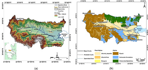
Sperchios Basin is an active asymmetric graben, bounded to the south by a major border fault system (Eliet and Gawthorpe 1995; Kilias et al. 2008; Whittaker and Walker 2015). Given the dominant tectonic activity in the area the catchment can be divided into two sections, in terms of morphological features and hydraulic behaviour. The northern, which is characterized by mild relief and lower mean elevation and the southern, that displays strong relief, steep slopes and diverse topography (Psomiadis et al. 2016). Active fault processes shape the tectonic geomorphology of the area and govern erosion and sedimentation processes along the basin. The bedrock is classified into three distinct lithological units (Ferrière 1977), representative of the western, south – south-eastern and north – north-eastern parts of the basin (Figure 1). Overall, the geological and geomorphological characteristics define the natural resources of the area, controlling soil type and water availability (runoff- infiltration), and by extension land use.

2.2. Datasets: technical parameters

2.2.1. The CLC project

CLC uses MMU of 25 ha for areal elements (fields, pastures, etc.), minimum width of 100 m for linear elements (linear urban constructions, linear vegetation zones, etc.) and MMU of 5 ha to identify LULC changes between surveys (https://land.copernicus.eu/pan-european/corine-land-cover). The inventory is organized in three hierarchical levels. The first level (global scale) includes five classes, the second 15 classes and the third and most detailed 44 classes (https://forum.eionet.europa.eu/nrc_land_covers/library/copernicus-2014-2020/pan-european-component/corine-land-cover-clc-2018/technical-guidelines/clc2018-nomenclature-guidelines).

CLC was initiated in 1985 (reference year 1990). Thus far, updates have been produced in the years 2000, 2006, 2012 and 2018, while the latest version is still under validation. The regular cycle information provided allow the demonstration of differences between succeeding records. Their results are comparable since the basic technical parameters of the inventory (MMU of 25 ha, minimum width of 100 m) have not changed from the beginning of the project (Büttner 2014).

2.2.2. The land parcel identification system

The LPIS is a spatial inventory of agricultural land in the form of RP. It comprises (CR No. 1306/2013), (i) digital database of aid applications and holdings, (ii) administrative system for recording and processing BD, (iii) identification and registration system and (iv) integrated control system to select farmers for on-the-spot inspection (http://www.europarl.europa.eu/meetdocs/2009_2014/documents/cont/dv/cocobufinal_/cocobufinal_en.pdf).

RPs are uniquely classified once registered in each MS’s GIS (Geographical Information System). In the context of the 2003 CAP reform, LPIS transcended from alphanumerical and without geospatial reference registry to a GIS-based one, utilizing very detailed geospatial data. Depending on the LPIS design of each MS, RP can be either cadastral parcel (CP), physical/topographical block (PB), farmer block (FB) or ilot or agricultural parcel (AP; Table 1) (European Court of Auditors 2016). PB is commonly used in the EU, given its temporal stability and ease of update. Yet, control procedures need to be more sophisticated. On the contrary, ilot and AP are considered appropriate options for administrative crosschecks, but their update is more complex and time-consuming (Grandgirard and Zielinski 2008) as, e.g. AP can be spatially and temporarily unstable due to crop rotation, abandonment of use and aggregation or subdivision of fields.

Table 1. Characteristics of the reference parcel types (Sagris et al. 2007; European Court of Auditors 2016).

	Cadastral parcel (CP)	Physical block (PB)	Farmer block (FB) or ilot	Agric. parcel (AP)
Features	One or more farmers	One or more farmers	Single farmer	Single farmer
	One or more crop groups	One or more crop groups	One or more crop groups	Single crop group
	Based on ownership – does not match agricultural patterns	Area bordered by certain features (ditches, etc.)	No natural boundaries
Data source	Cadastral; land register	Admin. classification	Farmer’s application	Farmer’s application
Timeframe	Not Applicable	Semipermanent	Multi-annual	Annual

2.2.3. The Greek LPIS

The Commission delegates the task of payment to beneficiaries to each MS, through accredited authorities (EC 2020). In Greece, such agency is the Payment and Control Agency for Guidance and Guarantee Community Aid (PCAGGCA).

Since the claim year 2009, PCAGGCA operates a state-of-the-art computerized cartographic database, complying with the technical standards of the new IACS (Kountouris 2009; Dimopoulou 2012). Specifically, the programme utilizes GIS techniques and recent orthophoto maps (1:5000; 1 m/pixel), developed based on recent Very High Resolution (VHR) satellite imagery. The project involves quality control, i.e. ortho-imagery correction, rectification and digitization – vectorization of ilot and sub-ilot (non-agricultural areas within the agricultural ilot) according to the natural blocks’ pattern. Disputable areas (normal changes in the agricultural terrain) and non-eligible elements (encroached vegetation, forests, man-made features such as roads and buildings) are detected and excluded following a twofold process. The latter comprises Computer Assisted Photo Interpretation (CAPI) of the rectified satellite images and on-site cross-checks (Kountouris 2009; Marakakis and Kalimeri 2018). All RP are assigned with an identification code that dictates basic attributes such as area and crop type, and the parcel’s location. The new system covers the entire Greek territory – even mountainous areas and rough landscapes with ongoing agricultural activity that occupy approximately 60% of the country, comprising 154 × 10⁴ ilot and 98 × 10⁵ sub-ilot (2012 values).

2.2.4. The Copernicus Sentinel-2 (S2)

The S2 mission supports the Community’s Copernicus programme. It comprises two identical satellites in the same orbit, 180° apart (http://www.esa.int/Our_Activities/Observing_the_Earth/Copernicus/Sentinel-2). Together they cover all Earth’s surface, providing imagery of high spatial (10 m) and temporal (5 days cycle, at the equator) resolution. Given its Multi-Spectral Imager (MSI) sensor and wide swath coverage (290 km width), it can deliver innovative and continuous land monitoring data. This satellite imagery is a unique tool for monitoring crop conditions and seasonal changes, LULC mapping, crop classification, yield prediction and so forth (Belgiu and Csillik 2018; Zoka et al. 2018; Psomiadis et al. 2019).

2.3. Datasets: attributes of utilized versions

2.3.1. CLC 2018

The latest 2018 version of CLC was used to depict the catchment’s LULC. The choice was based on its temporal ‘compatibility’ to the available IACS datasets and its improved ability to identify urban and peri-urban elements with >25 ha resolution. Specifically, small villages located within large plains or continuous cultivated areas, commonly met in the study site, are identified by using ancillary data, such as orthophotos and Google Earth imagery (https://land.copernicus.eu/usercorner/technical-library/clc2018technicalguidelines_final.pdf).

Fifteen level-2 classes were distinguished distributed among 967 features (Table 2). The basin is mostly comprised by ‘Semi-natural areas’ (classes 3.2, 3.3), occupying 626.6 km² (317 features). ‘Forests’ (class 3.1) is the second most expanded cover type, occupying 584.6 km² (208 features), dominating the mountainous parts of the catchment. Contrary, cultivated lands are prevalent at the lowlands, covering the hanging walls of the north dipping E-W trending active normal faults along the Kallidromo and Oiti mountain ranges, where the post-alpine loose sediments are developed parallel to the river’s horizontal axis (Figure 2b). Among them, ‘Arable land’ (class 2.1) is the most expanded class, occupying 231.8 km² (75 features), followed by ‘Heterogeneous agricultural areas’ (class 2.4), ‘Permanent crops’ (class 2.2) and ‘Pastures’ (class 2.3). ‘Artificial areas’ (classes 1.1‒1.4), ‘Wetlands’ (classes 4.1, 4.2) and ‘Water bodies’ (classes 5.1, 5.2) are less extended, having as dominant elements the city of Lamia, the coastal features of the Sperchios delta, and the Sperchios main watercourse, respectively.

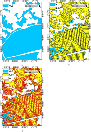
Figure 2. (a) CLC2018 classification; (b) Extent of agricultural areas within the basin.

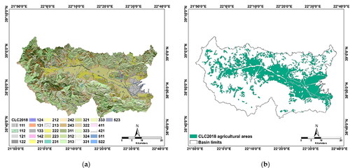
Table 2. CLC v. 2018 classification.

Level 1	No. of features	A (km^2)	A (%)	Level 2^a	No. of features	A (km^2)	A (%)	Level 3^b	No. of features	A (km^2)	A (%)
Artificial areas	87	50.73	2.78	1.1	70	34.34	1.88	111	1	3.66	0.20
								112	69	30.67	1.68
				1.2	6	9.71	0.53	121	4	5.21	0.29
								122	1	4.19	0.23
								124	1	0.31	0.02
				1.3	8	5.89	0.32	131	3	1.22	0.07
								133	5	4.67	0.26
				1.4	3	0.79	0.04	142	3	0.79	0.04
Agricultural areas	344	551.74	30.19	2.1	75	231.81	12.68	211	60	88.71	4.85
								212	13	140.31	7.68
								213	2	2.80	0.15
				2.2	42	87.93	4.81	222	5	35.39	1.94
								223	37	52.54	2.87
				2.3	5	2.77	0.15	231	5	2.77	0.15
				2.4	222	229.22	12.54	242	78	90.61	4.96
								243	144	138.61	7.58
Forest and seminatural areas	525	1211.1	66.27	3.1	208	584.62	31.99	311	67	173.30	9.48
								312	56	204.17	11.17
								313	85	207.15	11.33
				3.2	304	611.70	33.47	321	62	40.29	2.20
								322	19	53.97	2.95
								323	69	309.03	16.91
								324	154	208.41	11.40
				3.3	13	14.89	0.81	331	8	12.62	0.69
								333	5	2.27	0.12
Wetlands	5	7.14	0.39	4.1	1	0.92	0.05	411	1	0.92	0.05
				4.2	4	6.23	0.34	421	4	6.23	0.34
Water bodies	6	6.92	0.38	5.1	4	6.38	0.35	511	4	6.38	0.35
				5.2	2	0.55	0.03	522	1	0.25	0.01
								523	1	0.30	0.02
	967	1827.74	100		967	1827.74	100	Σ	967	1827.74	100

a 1.1: Urban fabric, 1.2: Industrial, commercial and transport units, 1.3: Mine, dump and construction sites, 1.4: Artificial, non-agricultural vegetated areas, 2.1: Arable land, 2.2: Permanent crops, 2.3: Pastures, 2.4: Heterogeneous agricultural areas, 3.1: Forests, 3.2: Shrub and/or herbaceous vegetation associations, 3.3: Open spaces with little or no vegetation, 4.1: Inland wetlands, 4.2: Coastal wetlands, 5.1: Inland waters, 5.2: Marine waters.

b 111: Continuous urban fabric, 112: Discontinuous urban fabric, 121: Industrial or commercial units and public facilities, 122: Road and rail networks and associated land, 124: Airports, 131: Mineral extraction sites, 133: Construction sites, 142: Sport and leisure facilities, 211: Nonirrigated arable land, 212: Permanently irrigated land, 213: Rice fields, 222: Fruit trees and berry plantations, 223: Olive groves, 231: Pastures, meadows and other permanent grasslands under agricultural use, 242: Complex cultivation patterns, 243: Land principally occupied by agriculture, with significant areas of natural vegetation, 311: Broad-leaved forest, 312: Coniferous forest, 313: Mixed forest, 321: Natural grasslands, 322: Moors and heathlands, 323: Sclerophyllous vegetation, 324: Transitional woodland/ shrub, 331: Beaches, dunes and sand plains, 333: Sparsely vegetated areas, 411: Inland marshes, 421: Coastal salt marshes, 511: Water courses, 522: Estuaries, 523: Sea and ocean.

Regarding the basin’s agricultural area distribution, i.e. level-3 classes (Figure 2a), ‘Permanently irrigated land’ has the greatest expansion, located (mainly) within the river valley and adjacent to its banks, capitalizing on the basin’s well-developed irrigation network. Of almost equal extent is the ‘Land principally occupied by agriculture, with significant areas of natural vegetation’ class. Its lands are mainly located at the ‘outskirts’ of the broader farmland area, within the highest elevation zones. ‘Rice fields’ are only met at the river delta, near its estuary. ‘Olive groves’ display a thinly disperse pattern, yet their vast majority is concentrated at the southern, south-eastern farmland limits. ‘Fruit trees and berry plantations’ and ‘Pastures’ occupy a minor part of the basin. The former is delimited to the watershed centre and within the river valley. The latter displays few manifestations at the centre of the watershed and its southern limits, within the highest altitudinal zones. Finally, ‘Non-irrigated arable land’ and ‘Complex cultivation patterns’ are randomly dispersed through the basin area.

2.3.2. FB or ilot

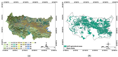
An upgraded edition of the ilot inventory was utilized to improve the coarse description of the CLC cultivated regions. Its default version, provided by PCAGGCA to the Agricultural University of Athens (AUA), was initially updated by Psomiadis (2010), and finalized during the programmes ‘Sperchios project’ (https://eeagrants.org/archive/2009-2014/projects/GR02-0014; http://www.eysped.gr/el/Documents/GR02.02.2.pdf). The update involved the introduction of additional classes towards a more comprehensive delineation. Specifically, classes 11–15 and 99 (Table 3) were introduced to improve the description of the forested regions, by differentiating forest types and specifying semi-natural areas. They are in accordance with the respective CLC ones, labelled according to the CLC2018 nomenclature (Table 2). Furthermore, the ‘Non-irrigated arable land’ class (code 44) was introduced to separate summer from winter crops, towards addressing the problems related to the seasonality of vegetation cover.

Table 3. Ilot classification.

Class	Use	No. of features	A (km2)	A (%)	CLC2018 match^1
10^a^, d	Forest	2526	460.70	25.21	312
11^b^, c	Mixed forest	123	34.56	1.89	313
12^b^, c	Coniferous forest	1718	298.38	16.33	311
13^b^, c	Mixed forest	79	22.72	1.24	313
14^b^, c	Sclerophyllous vegetation	1254	170.84	9.35	323
15^b^, c	Transitional woodland/shrub	135	36.12	1.98	324
20^a^, d	Urban	423	22.79	1.25	111
21^a^, e	Urban mixed	340	10.48	0.57	112
30^a^, d	Pastures	539	93.70	5.13	231
31^a^, e	Pastures mixed	1508	159.09	8.71	321
40^a^, d	Arable land	3495	169.20	9.26	212
41^a^, e	Arable land mixed	1139	80.05	4.38	212
44^b^, c	Nonirrigated arable land	1650	91.53	5.01	211
50^a^, d	Permanent crops	766	32.63	1.79	222
51^a^, e	Permanent crops mixed	471	25.35	1.39	212
60^a^, d	Olive groves	1005	34.09	1.87	223
61^a^, e	Olive groves mixed	340	15.50	0.85	223
70^a^, d	Vineyards	39	0.47	0.03	221
71^a^, e	Vineyards mixed	48	1.80	0.10	221
90^a^, d	Other	460	21.97	1.20	332^2
91^a^, d	Streets and water courses	702	30.73	1.68	511
95^b^, c	Water courses	24	4.26	0.23	511
98^b^, c	Estuaries	7	10.37	0.57	522
99^b^, c	Sparsely vegetated areas	1	0.13	0.01	333
Σ		18,792	1827.74	100

a Original.

b Update.

c See Table 2 footnote.

d Single patterns.

10: Forests, forested areas, shrubs, 20: Exclusively inhabited area, 30: (a) Pasture with coverage ≥ 30% of the ‘Pasture’ class (previous year delineation) and coverage ≥ 15% of declared for subsidy ‘Pasture’ class (current year delineation) or (b) Pasture with coverage ≥ 15% with of declared for subsidy ‘Pasture’ class (current year delineation), 40: Annual crops, 50: Permanent crops, 60: Olive groves of any given layout (normal, sparse, scattered), 70: Vineyards, 90: Non eligible uses, combined or individually considered, i.e. mineral extraction sites, salt pans, swamps, sport facilities, beaches, fallow lands, airports, bare rocks, 91: road network and adjacent features/areas, rivers, lakes, lagoons.

e Mixed patterns.

1 see Table 2 footnote, Table 4: column ‘CLC’.

2 332: Bare rock.

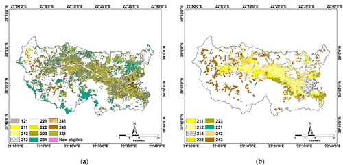
Twenty-four classes were distinguished (Figure 3a) distributed among 18,792 features (Table 3). The basin is mostly occupied by ‘Forests’ (codes 10–15, 99), covering 1023.4 km² (5836 features), i.e. 56% of its area. The latter are prevalent at the mountainous parts of the watershed where steep slopes and alpine rocks outcrop, evident to the tectonically uplifted footwall area of the Oiti and Kallidromo Mountains. ‘Agricultural areas’ (codes 30–71) is the second most expanded class, occupying 703.4 km² (11,000 features), i.e. 38.5% of the basin area (Figure 3b). Eleven categories were identified, distinguished into single (codes 30, 40, 44, 50, 60 and 70 – they may include additional eligible elements that occupy less than 10% of the total unit area) and mixed (codes 31, 41, 51, 61 and 71 – they include additional eligible elements that occupy more than 10% of the total unit area) patterns (Table 3).

Figure 3. (a) ILOT classification; (b) Extent of agricultural areas within the basin.

2.3.3. Beneficiaries’ declarations

A processed version of the 2018 edition of the BD inventory was compiled by the AUA, in the framework of the ‘Sperchios project’, to further improve the description of the ilot agricultural uses. Specifically, AUA used an anonymous subset of the 2018 version to avoid restrictions related to the farmer’s personal data. Furthermore, all common uses were dissolved to reduce computational load and homogenize the study area.

Eighty-five classes were distinguished (Figure 4b) distributed among 49,812 parcels (Table 4). The latter occupy 441.9 km², i.e. 24.2% of the basin area (Figure 4a). Their vast majority (49,478 parcels, 440 km², 99.3%) refer to single crop cultivations, while 334 parcels (2 km², 0.7%) represent co-cultivation systems, i.e. combinations of the individual crop types. Regarding the latter, and in the absence of more detailed information, the crop type mentioned first in the sequential order of each code is considered as the ‘dominant’ one, i.e. occupies the greater surface within each parcel, and the rest as complementary uses.

Figure 4. Crop type classification based on beneficiaries’ declarations (BD) for the reference period 2018: (a) Extent within the basin; (b) Enlarged detail near the basin outlet, labeled based on each parcel's crop type (as presented in Table 4).

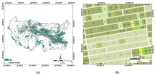
Table 4. BD 2018 classification.

Crop code	Crop type	Description^1	No. of parcels	%	Location^2	CLC^3	Ilot^4	A (km2)	%^c
1^a	Wheat	Durum wheat	1976	3.967	M1‒M9	211	40	17.520	0.959
1.38^b	Co-cultivation	Combination of respective types	3	0.006	M4, M8	211	41	0.017	0.001
2^a	Other cereal crops	Oats, barley, rye, soft wheat, sorghum	4200	8.432	M1‒M9, C1, C2	211	40	27.452	1.502
2.24^b	Co-cultivation	Combination of respective types	1	0.002	M4	211	41	0.008	0.000
2.38^b	»	»	18	0.036	M2‒M4, M8, M9	211	41	0.092	0.005
2.66^b	»	»	1	0.002	M8	241^6	41	0.002	0.000
2.8^b	»	»	2	0.004	M2	211	41	0.005	0.000
2.98^b	»	»	12	0.024	M4	243	41	0.091	0.005
3.1^a	Maize	−	547	1.098	M1‒M4, M7‒M9	211	44	6.124	0.335
3.1.38^b	Co-cultivation	Combination of respective types	3	0.006	M9	211	44	0.023	0.001
3.2^a	Maize silage	−	15	0.030	M2	211	44	0.068	0.004
4^a	Oil seeds	Sunflower	12	0.024	M3, M4	211	44	0.096	0.005
6^a	Fallow land	−	5801	11.646	M1‒M9, C1, C2	211	925	32.031	1.753
6.98^b	Co-cultivation	Combination of respective types	34	0.068	M4	243	925	0.294	0.016
7^a	Rice	−	528	1.060	M4, M5	213	40	8.332	0.456
8^a	Forage and fodder crops	Oats, clover, hay (alfalfa, barley, oats, vetch), dried peas, sorghum, soft wheat, durum wheat	8172	16.406	M1‒M9, C1, C2	211	40	60.791	3.326
8.98^b	Co-cultivation	Combination of respective types	15	0.030	M4	243	44	0.224	0.012
9^a	Pastures	−	5489	11.019	M1‒M9, C1, C2	231	30	152.323	8.334
11^a	Dried pulses (legumes)	Vetch, ervil, chickpeas, lentils	372	0.747	M1‒M9	211	44	2.400	0.131
11.24.38^b	Co-cultivation	Combination of respective types	1	0.002	M4	211	44	0.002	0.000
11.38^b	»	»	3	0.006	M3, M4	211	44	0.010	0.001
11.98^b	»	»	1	0.002	M4	243	44	0.027	0.001
12^a	Cotton	−	4003	8.036	M2‒M9	211	44	52.841	2.891
12.38^b	Co-cultivation	Combination of respective types	6	0.012	M3, M4, M7, M8	211	44	0.071	0.004
15^a	Olive groves (certified)	−	13,141	26.381	M1‒M9	223	60	48.991	2.680
15.21^b	Co-cultivation	Combination of respective types	3	0.006	M2, M4, M8	223	61	0.021	0.001
15.36.2^b	»	»	24	0.048	M2‒M4, M8, M9	223	61	0.058	0.003
15.36.3^b	»	»	3	0.006	M2, M4, M9	223	61	0.009	0.001
15.37.66^b	»	»	1	0.002	M4	223	61	0.001	0.000
15.38^b	»	»	7	0.014	M4, M7, M8	223	61	0.034	0.002
15.66^b	»	»	14	0.028	M4, M5, M7, M8	223	61	0.052	0.003
15.66.67^b	»	»	3	0.006	M3, M4, M8	223	61	0.014	0.001
15.8^b	»	»	7	0.014	M1, M4, M5, M7, M8	223	61	0.027	0.001
15.98^b	»	»	63	0.126	M4	243	61	0.237	0.013
16^a	Energy crops	Sunflower, rapeseed	129	0.259	M2‒M5, M8, M9	211	44	1.732	0.095
16.98^b	Co-cultivation	Combination of respective types	1	0.002	M4	243	44	0.070	0.004
17^a	Tobacco	−	38	0.076	M2, M3, M8	211	44	0.326	0.018
18^a	Tomatoes (for processing)	−	4	0.008	M3, M9	212	40	0.051	0.003
19^a	Citrus fruits (for processing)	No info	1	0.002	M4	222	50	0.001	0.000
20.2.66^b	Co-cultivation	Combination of respective types d	1	0.002	M8	222	51	0.004	0.000
21^a	Nut crops	Walnut, almond, peanut, hazelnut	2117	4.250	M1‒M9, C1, C2	222	50	15.235	0.834
21.24.38^b	Co-cultivation	Combination of respective types	1	0.002	M7	241^6	51	0.004	0.000
21.38^b	»	»	2	0.004	M4, C1	241^6	51	0.008	0.000
21.38.66^b	»	»	1	0.002	C1	241^6	51	0.001	0.000
21.45.2^b	»	»	9	0.018	M1, M4, M8, M9	222	51	0.053	0.003
21.45.2.66^b	»	»	3	0.006	M2, M4, M7	222	51	0.012	0.001
21.45.2.67^b	»	»	2	0.004	M7, M8	222	51	0.009	0.000
21.66^b	»	»	3	0.006	M7	222	51	0.009	0.001
21.66.67^b	»	»	2	0.004	M4, M7	222	51	0.010	0.001
21.67^b	»	»	5	0.010	M3, M4, M6, M8, M9	222	51	0.081	0.004
21.8^b	»	»	9	0.018	M4, M7	241^6	51	0.087	0.005
21.98^b	»	»	3	0.006	M4	243	51	0.054	0.003
24^a	Potatoes (for starch production)	−	71	0.143	M1‒M5, M7‒M9, C1, C2	211	40	0.153	0.008
24.38^b	Co-cultivation	Combination of respective types	10	0.020	M4, M7	211	41	0.047	0.003
24.98^b	»	»	1	0.002	M4	243	41	0.004	0.000
25^a	Seed crops	Alfalfa, vetch	45	0.090	M2, M4, M6, M8	211	44	0.373	0.020
36.2^b	Vineyards for wine production	−	492	0.988	M1‒M9	221	70	1.215	0.066
36.3^b	Vineyards for consumer grapes	−	87	0.175	M1‒M9	221	70	0.153	0.008
37^a	Other citrus crops	Grapefruit; orange; lemon; mandarin; other trees	3	0.006	M5, M9	222	50	0.001	0.000
37.66^b	Co-cultivation	Combination of respective types	1	0.002	M4	222	51	0.001	0.000
37.66.67^b	»	»	1	0.002	M7	222	51	0.000	0.000
37.67^b	»	»	1	0.002	M4	222	51	0.001	0.000
38^a	Vegetables	Beans, potatoes, tomatoes, onions, fresh greenhouse vegetables, watermelons, cauliflowers, industrial vegetables (green beans, okras, peas), melons, asparagus, peppers, lettuce, artichokes, cucumbers	471	0.946	M1‒M9, C1, C2	211	44	1.682	0.092
38.39^b	Co-cultivation	Combination of respective types	3	0.006	M4, M9	243	44	0.008	0.000
38.8^b	»	»	17	0.034	M3, M7‒M9	211	44	0.058	0.003
39^a	Vegetables (under cover)	−	42	0.084	M3, M4, M6‒M9	212	40	0.061	0.003
40^a	Floriculture	Flowers and ornamental plants, flowers and ornamental plants (under cover; greenhouse), gardening plants and other floriculture outdoor plants	9	0.018	M3, M4, M8	211	44	0.026	0.001
40.45.3^b	Co-cultivation	Combination of respective types	1	0.002	M2	211	44	0.001	0.000
41^a	Aromatic plants	Oregano, various	37	0.074	M1‒M4, M7‒M9	211	44	0.140	0.008
42^a	Uncultivated land	−	115	0.231	M3‒M5, M7, M9	231	925	0.305	0.017
45.1^b	Other crops	Tree crops-various, fallow land	78	0.157	M1‒M9	222	50	0.381	0.021
45.2^b	Other crops – Tree crops	Chestnuts, cherries, sour cherries, pears, apples, kiwi, pomegranates, plums, quinces, peaches, nectarines, apricots, damsons	561	1.126	M1‒M5, M7‒M9, C2	222	50	4.019	0.220
45.2.66^b	Co-cultivation	Combination of respective types	4	0.008	M4, M7, M9	222	51	0.020	0.001
45.2.66.67^b	»	»	9	0.018	M4, M7‒M9	222	51	0.028	0.002
45.2.67^b	»	»	2	0.004	M4, M5	222	51	0.047	0.003
45.3^b	Nurseries	Nurseries of floriculture plants, nurseries of fruit trees and fruit shrubs	17	0.034	M2, M4, M8	211	44	0.084	0.005
47^a	Snail farms	−	2	0.004	M8	121	90	0.008	0.000
48^a	Renewable energy installation areas	No info	51	0.102	M2‒M9	121	90	0.195	0.011
49^a	Other crops-forest trees	Chestnuts, cherries, sour cherries, pears, apples, kiwi, pomegranates, plums, quinces, peaches, nectarines, apricots, damsons	104	0.209	M3‒M5, M7‒M9	222	50	1.696	0.093
66^a	Tree crops	Chestnuts, cherries, sour cherries, pears, apples, kiwi, pomegranates, plums, quinces, peaches, nectarines, apricots, damsons	627	1.259	M2‒M5, M7‒M9	222	50	2.728	0.149
66.67^b	Co-cultivation	Combination of respective types	17	0.034	M4, M7, M9	222	51	0.067	0.004
67^a	Apple trees	−	105	0.211	M2‒M5, M7‒M9	211	50	0.320	0.018
68^a	Asparagus	−	1	0.002	M4	211	44	0.007	0.000
98^a	Non-eligible land	−	9	0.018	M4	−	90	0.021	0.001
99^a	Non-eligible land	−	6	0.012	M4	−	90	0.041	0.002
			49,812	100.00				441.93	24.18

^aSingle crop type.

^bMultiple crop types.

^cEstimated as fraction of the total basin area, i.e. 1827.74 km².

^dPrimary use: 20.2: Peaches (for processing).

¹Source: https://it.opekepe.gr/aggregate/. . . . . . . , accessed on 06/03/2020.

²Municipalities: M₁: Ag. Georgios, M₂: Makrakomi, M₃: Leianokladi, M₄: Lamia, M₅: Stylida, M₆: Molos, M₇: Gorgopotamos, M₈: Ypati, M₉: Sperchiada /Communities: C₁: Pavliani, C₂: Tymfristos.

³CLC2018 Level 3 match (see Table 2 footnote).

⁴Ilot classification match (see Table 3 footnote).

⁵Class 92: abandoned arable land (past seasons’ annual crops unit, identified by the non-utilized regular shape agricultural parcels included to it).

⁶ 241: Annual crops associated with permanent crops.

The most widespread LULC type is ‘Pastures’. It covers the mountainous parts of the basin, with only a minor portion resting over the valley at the lowlands. ‘Forage and fodder crops’ is the second most widespread type. ‘Cotton’ fields, ‘Cereal’ and ‘Olive groves’ share similar extent. Cotton is mainly cultivated at the lower central part of the valley and the river delta. Olive groves are more commonly met at the ‘outskirts’ of the broader farmland area, within relatively higher elevation zones. Forage and fodder crops and cereals do not display a specific pattern and are randomly dispersed throughout the cultivated area. ‘Nut crops’ are also a significant source of income in the region. They are mainly found at the central part of the basin, in low to medium altitudinal zones. ‘Rice fields’ are only found in the river delta, as in the case of the CLC inventory. ‘Fallow land’ parcels display random distribution. Finally, only 15 parcels are classified as ‘Non-eligible’ for subsidy land.

The parcel ranking per crop type does not coincide to the respective per area one. For example, although olive groves occupy only 2.7% of the total basin area, they are distributed among 13,141 (26.4%) parcels. Contrary, pastures occupy 8.3% of the basin area, yet they are only distributed among 5489 (11%) parcels.

2.3.4. Sentinel-2 (S2) imagery

Four cloud free and atmospherically corrected (processing level 2A) S2 images, representative of the 2018 winter and summer crop development stages, covering 60% of the total basin area and 90% of its cultivated lands, were acquired, to distinguish the existing crop types and assist the evaluation of the declared parcels dataset correctness (Table 5 and Figure 5). The images were downloaded free of charge from the European Space Agency (ESA) portal (https://scihub.copernicus.eu/). The colour patterns are representative of the reflectance properties of each crop and soil type, indicative of the different development stage’s/season’s vegetation vitality and canopy extend.

Figure 5. False Color Composites (B11-Short Wave Infrared, B8-Near Infrared and B2-Blue bands as RGB) of Sentinel-2 images acquired on: (a) 5 December 2017, winter; (b) 14 April 2018, spring; (c) 03 July 2018, summer; (d) 16 September 2018, autumn.

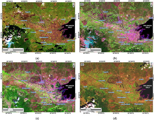
Table 5. Satellite image dataset.

Satellite system	Instrument	Image code/source	Acquisition	Season
Sentinel-2	MSI	S2A_MSIL2A_20171205T092341_N0206_ R093_T34SFJ_20171205T114023	05/12/2017	Winter
		S2A_MSIL2A_20180414T092031_N0207_ R093_T34SFJ_20180414T104532	14/04/2018	Spring
		S2A_MSIL2A_20180703T092031_N0208_R093_ T34SFJ_20180703T121025	03/07/2018	Summer
		S2B_MSIL2A_20180916T092019_N0208_ R093_T34SFJ_20180916T121224	16/09/2018	Autumn

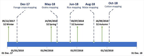
Figure 6 indicates the time periods when each satellite image was acquired, in relation to the crop development stages of key crop types in the study area.

Figure 6. Graphical representation showing the timetable between the acquisition date of the satellite images and the development stages of key crops in the study area.

Pre-processing involved image resampling, subset and masking. Specifically, resolution was resampled to 10 m, using the B2 band of S2 as panchromatic image and employing the fusion method (‘Resampling’ tool) of the Sentinel Application Platform (SNAP) provided by the ESA (http://step.esa.int/main/toolboxes/snap, accessed on 09/08/2020). This is because S2 operates on 13 different bands at spatial resolution of 10 (4 bands; B2, B3, B4 and B8), 20 (6 bands; B5, B6, B7, B8A, B11 and B12) and 60 (3 bands; B1, B9 and B10) m. Moreover, given the size of the study area, there was no need to process the entire image – thus, it was clipped for computational reasons, while pixels outside the basin limits were excluded. Finally, the stack (collocation) of 10 spectral bands for each date was executed by excluding bands 1 (coastal aerosol), 9 (water vapor) and 10 (cirrus).

2.4. Validation of the BD using S2 data classification

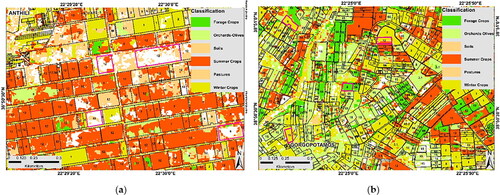
The classification image created (Figure 7) was used for the validation of the farmers’ declared crops database.

Figure 7. Characteristic classified areas representing the validation of the declared parcels of the areas: (a) Next to Anthili village; (b) Next to Gorgopotamos village. Ping polygons show the incorrectly parcels.

Supervised classification was performed using the RF classifier (Breiman 2001). RF is an ensemble (Rokach 2010) tree-based machine learning algorithm. It combines Ho’s Random Selection of Features concept (Ho 1995) and Breiman’s ‘Bagging’ technique, a joint term that refers to bootstrapping followed by aggregation (Breiman 1996). RF was run utilizing the RF classification toolbox of the SNAP.

The reference samples were collected in 2018 (from the winter of 2017 until the autumn of 2018) after extended fieldwork based on random stratified sampling. The farmers’ declared parcels, aided by very high-resolution aerial orthophotos and Google Earth images, served as guide towards acquiring a satisfactory amount of each of the selected classes (Psomiadis et al. 2020). Then, the samples were split into two sets of disjoint training (420; 60%) and validation (280; 40%) points. Using the first training set and 12 classes, a two-step classification procedure was followed. The first step comprised a broad differentiation between crops, mixed areas (of natural vegetation and crops) and forest, water and built-up classes. On the second step, crops were further classified into summer and winter arable types, permanent crops (orchards), olive groves, vineyards and pastures.

Subsequently, the accuracy of the classification map was assessed by using the second validation set. The results were attested using the Overall Accuracy (OA), producer’s accuracy (PA) and user’s accuracy (UA) metrics (Congalton 1991) and the Kappa coefficient (Cohen 1960) that measures the agreement between the observed and predicted or inferred classes for cases in the testing dataset.

Finally, the BD dataset was validated utilizing the classified image with the higher accuracy. More specifically, 250 parcels were randomly selected, well-distributed and inclusive of all classified crop types and the image-BD agreement was examined. In addition, a final cross-validation was made by checking, in situ, 80 parcels, selected by those used for validation purposes.

2.5. Methodological framework

The methodology followed is outlined by the workflow ‘Problem identification – Literature review – Hypothesis – Experimental testing – Data analysis – Conclusions’. The limitations of CLC, especially those of its agricultural uses (e.g. temporal stationarity, low spatial resolution, broad and rather simplified grouping of classes), were initially identified and documented. Subsequently, international literature was thoroughly reviewed, investiging for potential solutions. The next step was to develop an innovative proposal towards addressing these problems. Then, the Sperchios River Basin in Greece was selected as test site (given the in-depth knowledge of its specific characteristics, the availability of the relative data and the overall importance of the river as a regional growth and development driver) and research evolved towards evaluating the hypothesis introduced. The final steps of the study comprised the analysis of the data, the interpretation of the results and the presentation of conclusions.

In particular, the core concept of this research effort was to minimize, eliminate, if possible, the shortcomings of the CLC agricultural classes by utilizing more detailed LULC datasets. In the attempt to exploit their advantages, national and pan-European datasets were coupled developing hybrid geospatial layers. These layers derived from the sequential incorporation and progressive update of the individual datasets available, as: BD → BD-ilot → BD-ilot-CLC. The fusion was implemented in a GIS environment, utilizing the ArcGIS suite (10.7.1 version).

Preparatory work involved the acquisition and pre-processing of seasonal remote sensing data of high spatial resolution (S2 imagery; they provide the same resolution as CLC), which were used to validate (and rectify if necessary) the realism of the BD database.

Among the three datasets used, only the BD map was evaluated, subject to the most frequent and significant accuracy errors, i.e. in terms of farmland location/delimitation, crop type description and cultivation area, as its development relies primarily on farmer applications. The CLC2018 and ilot maps were considered accurate, as to the information they provide in their initial (default) form/resolution. BD validation further aided to the assignment of the winter/summer crop status, given the great number of misleading or non-updating features (Soulis et al. 2020). Supervised classifications were performed using the Random Forest (RF) classifier, and the values of appropriate statistical measures employed confirmed the reliability of the dataset. Once its correctness was attested (decision was made polygon-by-polygon considering the reference parcels and a random sampling of a few more for each class) the declared farmlands became eligible for inclusion in the new map.

Then, the individual farmlands of the BD registry were incorporated in the agricultural parcels of the regional ilot map, towards upgrading its cultivated areas. The gaps in the agricultural polygons of the updated ilot layer, owed to non-eligible or not declared lands and delimiting or discontinuity elements, were patched by the BD records. This intermediate product (ilot-BD) with the highly detailed agricultural components can be used as an individual LULC map in various applications, constituting an additional benefit of this effort.

Subsequently, the farmland segments of the novel ilot-BD layer were integrated to the respective CLC classes, developing the next generation object-oriented (i.e. farmland based) LULC map of the study area. This highly detailed layer in terms of cultivated land description served as the foundation on which the CLC2018 inventory expanded, to fill in the gaps at non-agricultural regions and ‘patch’ under-described or undescribed agricultural lands within the embedded ilot polygons. Furthermore, this appendence addressed classification errors of the CLC inventory, e.g. cultivated lands mixed with forest areas, such as the 243 (Land principally occupied by agriculture, with significant areas of natural vegetation) and 244 (Agroforestry areas) classes, by separating the cultivated farmlands.

The CLC2018 nomenclature provided the foundation, on which the classification processing of the three layers was based. Since the ilot and BD datasets entail different crop categories, they had to be reclassified according to the target map registry, to surpass inconsistencies and make the comparison and operations between them feasible. The relevance of their components led to a straightforward matching of all crop types and cultivation systems. It is noted that during the development of the upgraded ilot map, i.e. ilot-BD layer incorporation stage, the BD records were also reclassified, this time according to the ilot features.

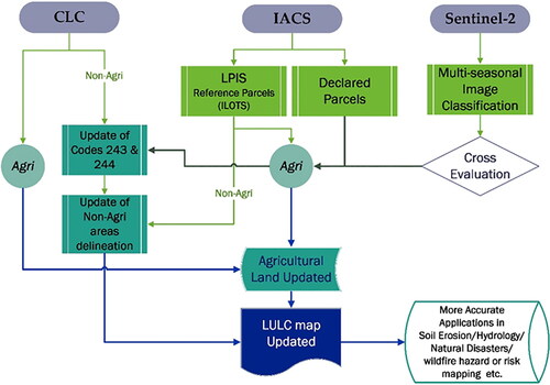
The flowchart (Figure 8) presents schematically the methodology followed towards the development of the new land cover map of the basin.

Figure 8. Methodology flow chart.

The sequential incorporation of the hybrid datasets/layers is briefly presented in Figure 9. One can easily notice the greater extent and more detailed description of the cultivated land in the form of RP in the CLC-ilot map, compared to the initial, coarse CLC delineation, the improved description of the agricultural ilot in the CLC-ilot-BD map and the remaining gaps in a number of those polygons. The latter indicate either the absence of declared farmlands or the presence of non-eligible elements.

Figure 9. Sequential integration of hybrid LULC layers towards the final object-oriented map of the Sperchios River basin – area adjacent to the new riverbed (old spillway) near the river Delta: (a) CLC; (b) CLC-ILOT integration; (c) CLC-ILOT-BD integration.

3. Results

3.1. BD validation

The classification OA was estimated at 83.3% (140 correctly classified parcels divided to 168 total reference parcels), which is considered much better than the accuracy of the BD, which usually is close to 70–75% or less (Soulis et al. 2020), and the Kappa coefficient at 0.82. The PA index for the ‘orchards-olives’, ‘summer-arable’ and ‘winter-arable’ crops acquired very high values of 92.3%, 94.6% and 85%, respectively. These classes also displayed high UA values of 85.7%, 89.7% and 91.9%, respectively. The PA and UA values for the ‘bare soils’, ‘pastures and forage land’ classes were lower, varying from 66.7% to 75% and from 66.7% to 80%, respectively. Overall, the values of the statistical measures employed confirmed the reliability of the classified image.

Regarding the validation of the dataset, i.e. the image-BD agreement examination, the results demonstrated a 91.2% coincidence (228 out of 250 parcels) between them. In addition, the cross validation showed that 79 out of 80 parcels from the validation group were correct, indicating the high accuracy of the process. Validation results displayed satisfactory accuracy; thus, no further modifications were required.

3.2. The intermediate upgraded ilot map

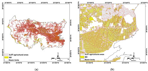
The ilot agricultural classes (Figure 10) cover an additional surface of 261.5 km² (703.4 km²) in comparison to the BD delineation (441.9 km²), implying a 59.2% increase. The divergence is due to gaps within each ilot, resulting by the presence of non-eligible or not declared farmlands, and the physical boundaries, e.g. roads, etc., that separate the RP. Remote farmlands of the BD dataset can be found at mountainous regions and rough landscapes with ongoing agricultural activity, mostly at the southern part of the basin. Spatial deviations, i.e. occupied space, are also detected at its northern and western part, where there is surplus of ilot polygons at the highest altitudinal zones.

Figure 10. ILOT-BD 2018 overlap: (a) Spatial extent divergence within the basin; (b) Enlarged detail near the basin outlet.

The divergence between the LULC pattern of the two maps is presented in Figure 11. For consistency reasons the BD map nomenclature was reclassified, matching each crop type to a relevant ilot group based on its comprising features (Table 6). The process was straightforward for both single crop type and co-cultivation systems.

Figure 11. ILOT-BD 2018 pattern divergence: (a) ILOT pattern; (b) BD 2018 pattern.

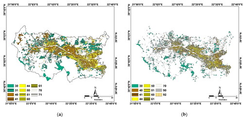
Table 6. Ilot-BD 2018 match.

Ilot code	Ilot description	BD^a crop codes	No. of parcels	%	A (km^2)	%^b
30	Pastures	9	5489	11.02	15.32	8.33
40	Arable land	1, 2, 7, 8, 18, 24, 39	14,993	30.10	114.36	6.26
41	Arable land mixed	1.38, 2.24, 2.38, 2.66, 2.8, 2.98, 24.38, 24.98	48	0.10	0.27	0.02
44	Nonirrigated arable land	3.1, 3.1.38, 3.2, 4, 8.98, 11, 11.24.38, 11.38, 11.98, 12, 12.38, 16, 16.98, 17, 25, 38, 38.39, 38.8, 40, 40.45.3, 41, 45.3, 68	5747	11.54	66.39	3.63
50	Permanent crops	19, 21, 37, 45.1, 45.2, 49, 66, 67	3596	7.22	24.38	1.33
51	Permanent crops mixed	20.2.66, 21.24.38, 21.38, 21.38.66, 21.45.2, 21.45.2.66, 24.45.2.67, 21.66, 21.67, 21.8, 21.98, 37.66, 37.66.67, 37.67, 45.2.66, 45.2.66.67, 45.2.67, 66.67	76	0.15	0.50	0.03
60	Olive groves	15	13,141	26.38	48.99	2.68
61	Olive groves mixed	15.21, 15.36.2, 15.36.3, 15.37.66, 15.38, 15.66, 15.66.67, 15.8, 15.98	125	0.25	0.45	0.03
70	Vineyards	36.2, 36.3	579	1.16	1.37	0.08
90	Other	47, 48, 98, 99	68	0.14	0.26	0.01
92	Abandoned arable land	6, 6.98, 42	5950	11.94	32.63	1.79
			49,812	100.00	441.93	24.18

a Beneficiaries’ declarations.

b Estimated as fraction of the total basin area, i.e. 1827.74 km².

Most single type crops (14,993 parcels; 30%; 7 crop codes) belong in the 40 class (‘Arable land’), occupying an area of approximately 114 km², followed by those (13,141 parcels; 26.4%; 1 crop code) grouped in the 60 class (‘Olive groves’), occupying an area of approximately 49 km². It is noteworthy that the ilot 31 class (‘Pastures mixed’) does not appear in the BD delineation, while the 71 (‘Vineyards mixed’), 90 (‘Other’), 92 (‘Abandoned arable land’) classes do not appear in the ilot map. Moreover, although most crop codes were grouped in class 51, the latter was comprised by only 76 parcels (0.2%), occupying merely 0.5 km² of land. In terms of spatial extent, the 40 class covered the greater part of the delineated area, followed by the newly introduced 44 class (‘Non-irrigated arable land’).

The upgraded ilot map (Figure 12), including both the newly developed agricultural uses and the original non-agricultural ones, is classified according to the CLC2018 nomenclature (Tables 2–4).

Figure 12. (a) New ILOT map with upgraded agricultural uses, after the incorporation of the individual farmlands provided by the BD dataset; (b) Enlarged detail near the basin outlet.

3.3. The new LULC map

The new LULC map comprises forested (non-agricultural) regions described only by CLC features (the information provided for these regions, i.e. mainly the differentiation between deciduous and evergreen forests, is considered adequate, given their low or even almost null spatial variability), and agricultural areas described by CLC features, ilot polygons and BD parcels. Thus, the forested regions retain the same resolution as the parent CLC2018 map. The agricultural areas resolution differentiates to those that do not include declared farmlands and to those that do. Regarding the former, the size of their RP, according to the Greek LPIS system, varies from approximately 20–40 ha for the ‘Olive groves’ and ‘Vineyards’ classes to 40–80 ha for the ‘Arable land’ and ‘Permanent crops’ ones, depending on the presence and extent of physical boundaries that separate them, such as roads. Regarding the later, the RP size is defined by the respective size of each declared parcel, ranging from 2 to 4 ha (mean representative value for the Greek ownerships).

The agricultural land (Table 7; column ‘Level 3′; classes 112, 211–243, non-eligible and 321) of the upgraded ilot map (Figure 13) covers an additional surface of 286.9 km² (838.7 km²; 61,139 features) in comparison to the CLC2018 delineation (Table 3; 551.7 km²; 344 features), implying a 52% increase. Following the incorporation of the two layers, the rural areas of the final LULC inventory (Table 8; 725.7 km²; 59,531 features) cover an additional surface of 174 km² in comparison to the CLC2018 delineation, implying a 31.5% increase. The huge difference between their comprising features is owed to the MMU of the CLC (25 ha), and the fact that the farmlands of the final LULC, originating from the BD dataset with mean parcel/ownership area ranging from 2 to 4 ha, comprise highly fragmented cultivated land belonging to different owners.

Figure 13. Upgraded ILOT-CLC2018 overlap: (a) Spatial extent divergence within the basin; (b) Enlarged detail near the basin outlet.

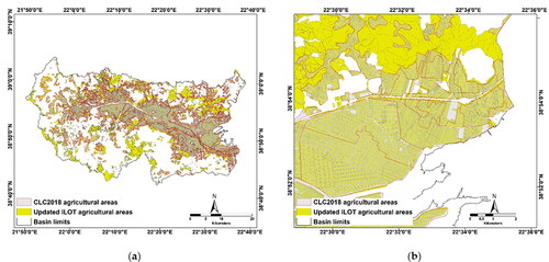
Table 7. LULC classification of the Sperchios River basin after the upgraded ilot-CLC2018 overlap.

Level 1	Level 3	No. of features^f	A (km2)	A (%)	No. of features	A (km2)	A (%)	Ilot^1	BD^2
Artificial areas	111^a	424	22.57	1.23	872	34.11	1.87
	112^a	386	10.92	0.60
	121^a^, d	53	0.20	0.01				‒	48
	122^a	1	0.06	0.00
	131^a	3	0.08	0.00
	133^a	2	0.10	0.01
	142^a	3	0.18	0.01
Agricultural areas	211^a^, d	27,688	233.67	12.78	59,531	725.69	39.70	44	1, 1.38, 2, 2.24, 2.38, 2.8, 3.1, 3.1.38, 3.2, 4, 6, 8, 11, 11.24.38, 11.38, 12, 12.38, 16, 17, 24, 24.38, 25, 38, 38.8, 40, 40.45.3, 45.3, 68
	212^a^, d	5146	101.90	5.57				40, 41, 51	18, 39
	213^a^, d	4422	41.00	2.24				50	19, 20.2.66, 21, 21.45.2, 21.45.2.66, 21.45.2.67, 21.66, 21.66.67, 21.67, 37, 37.66, 37.66.67, 37.67, 45.1, 45.2, 45.2.66, 45.2.66.67, 45.2.67, 49, 66, 66.67, 67
	221^b^, d	666	2.90	0.16				‒	36.2, 36.3
	222^a^, d	528	8.33	0.46				‒	7
	223^a^, d	14,568	72.25	3.95				60, 61	15, 15.21, 15.36.2, 15.36.3, 15.37.66, 15.38, 15.66, 15.66.67, 15.8
	231^a^, d	6148	202.21	11.06				30	9, 42
	241^c^, d	14	0.10	0.01				‒	2.66, 21.24.38, 21.38, 21.38.66, 21.8
	242^a^, e	64	4.68	0.26				‒	‒
	243^a^, d	272	58.58	3.20				‒	2.98, 6.98, 8.98, 11.98, 15.98, 16.98, 21.98, 24.98, 38.39
	Non-eligible^c	15	0.06	0.00				‒	98, 99
Forest and seminatural areas	311^a	66	158.45	8.67	2481	1023.49	55.99
	312^a	55	193.53	10.59
	313^a	85	185.74	10.16
	321^a	1568	112.76	6.17				31	‒
	322^a	19	8.59	0.47
	323^a	65	189.82	10.38
	324^a	152	154.18	8.44
	331^a	5	1.57	0.09
	332^b	460	18.06	0.99
	333^a	6	0.78	0.04
Wetlands	421^a	4	0.07	0.00	4	0.07	0.004
Water bodies	511^a	728	34.58	1.89	737	44.50	2.43
	522^a	8	9.76	0.53
	523^a	1	0.16	0.01
	Σ	63,625	1827.74	100	63,625	1827.74	100

a See Table 2 footnote.

b See Table 3.

c See Table 4.

d See Table 4, column ‘crop codes’ for the crop types included in each class.

e Derives directly from the CLC classification, not comprising ilot or BD parcels.

f Parcels when referring to the Agricultural areas.

1 Source of agricultural use, see Table 3.

2 Source of agricultural use, see Table 4.

Table 8. Deviations between CLC2018 and final LULC map.

Level 1	CLC2018		Final LULC		Deviation^a		Deviation^a
	No. of features	A (km^2)	No. of features	A (km^2)	No. of features	%	Area (km^2)	%
Artificial areas	87	50.73	872	34.11	785	902.30	–16.62	–32.76
Agricultural areas	344	551.74	59,531	725.69	59,187	17,205.52	173.95	31.53
Forest and seminatural areas	525	1211.1	2481	1023.49	1956	372.57	–187.72	–15.50
Wetlands	5	7.14	4	0.07	–1	–20.00	–7.07	–99.01
Water bodies	6	6.92	737	44.50	737	12,283.33	37.58	542.84

a The minus sign shows decrease against the initial values.

The spatial deviation between the two datasets is more evident at the cultivated mountainous regions of the basin, and mainly at its northern and southern parts. Major differences derive from the extent and locality of some classes. For example, in the CLC inventory ‘Pastures’ occupy only a small area, limited at the centre of the watershed and its southern borders, while in the upgraded ilot map is the most widespread use, dispersed over the mountainous regions. Yet, it must be underlined, that in the ‘coinciding zone’, several records display common presence and similar distribution, e.g. ‘Rice fields’ can only be found at the river delta, near the basin estuary; ‘Olive groves’ are met at the ‘outskirts’ of the main farmland area limits, etc. Moreover, there is a profound alteration in the depiction pattern of the catchment’s rural areas, transcending from coarse description (CLC) to highly accurate resolution (upgraded ilot).

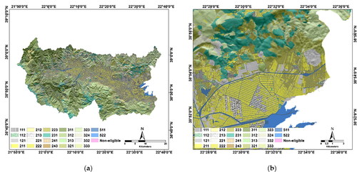
To further investigate the divergence of their patterns (Figure 14), the upgraded ilot map was reclassified, based on the matching of its comprising classes to the respective CLC ones (Tables 3 and 5). As in the case of the ilot; BD overlap (Figure 10), the ilot 121 (‘Industrial or commercial units and public facilities’), 221 (‘Vineyards’), 241 (‘Annual crops associated with permanent crops’) and 321 (‘Natural grasslands’) classes do not appear in the CLC delineation, while the 242 (‘Complex cultivation patterns’) does not appear in the map.

Figure 14. Upgraded ILOT-CLC2018 pattern divergence: (a) Upgraded ILOT pattern; (b) CLC2018 pattern.

In the final map (Table 7), most features (27,688; 13.8%) were grouped in the 211 class (‘Non-irrigated arable land’), occupying approximately 234 km², followed by those (14,568; 4%) grouped in the 223 class (‘Olive groves’), covering approximately 72 km². Additionally, apart from the apparent prevalence of the 211 class in terms of comprising features population and occupied basin space, the respective rankings among the remaining classes do not coincide, e.g. class 223 ranks second in comprising features but only fourth in area extent.

Overall, thirty-two level-3 classes were distinguished in the basin, distributed among 63,625 elements (Table 7). The basin is mostly comprised by ‘Forests and semi-natural areas’ (1023.5 km², 56% of its area). The second most common use is agriculture (∼46% of the basin area) with the respective ‘Agricultural areas’ class occupying 838.7 km² (61,139 features). The origin of each agricultural use is presented in the columns ‘ilot’ and ‘BD’ of Table 7. The three remaining classes cover a minor portion of the catchment. The final LULC map of the Sperchios River basin is presented in Figure 15.

Figure 15. LULC map of the Sperchios River basin after the upgraded ILOT-CLC2018 overlap.

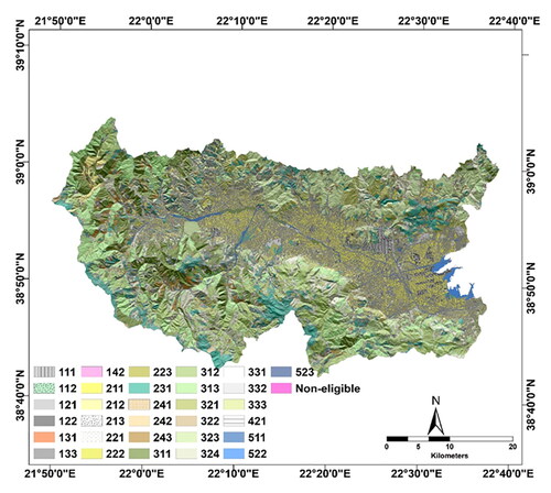
In terms of spatial extent, the level-1 classes of the CLC and final LULC share the same ranking (Table 8). In the final map, the area of the classes ‘Artificial areas’, ‘Forest and semi-natural areas’ and ‘Wetlands’ was reduced, while that of the ‘Agricultural areas’ and ‘Water bodies’ classes was increased. ‘Forests and semi-natural areas’ remained the dominant type in the basin, and ‘Agricultural areas’ is still the second most expanded class. Moreover, there is a n-fold increase in the number of agricultural features. Furthermore, in the new LULC delineation, the increase of the cultivated lands area (the new map comprises ∼175 km² of additional land, that was probably registered as ‘Forests and semi-natural areas’ in the CLC2018) is almost equal to the area decrease (∼190 km²) of the respective land type.

4. Summary

A GIS-based database with supporting technical data (attribute tables), a report on all stages of the project, and LULC statistics per dataset (CLC2018, LPIS, BD) and stage (LPIS-BD integration, final LULC map development) were produced. Additional benefits (deliverables) were, the: (i) evaluated (in terms of realism) BD inventory, that helped to describe more comprehensively the seasonal variations of vegetation cover by distinguishing summer from winter crops, (ii) development of an intermediate ilot-BD map, which can be used individually in various applications, (iii) harmonization of the IACS inventories with the CLC nomenclature, that can serve as matching guideline for similar future ventures.

The statistical overview outlines that the number of comprising elements (and classes) of the initial datasets were a function of their spatial detail level, i.e. the higher the detail (BD > ilot > CLC2018) the greater their number (49,812 BD parcels/85 classes > 18,792 ilot polygons/24 classes > 967 CLC features/15 classes). Furthermore, the agricultural uses of the upgraded ilot map appeared increased by 52% compared to the CLC2018 ones, covering an additional surface of 286.9 km². Besides, the cultivated lands of the final LULC map extended to a surplus area of 174 km² in comparison to the CLC2018 delineation, indicating a 31.5% increase. The n-fold rise in the number of the respective features (59,531 against 344) is due to the divergence between the CLC MMU (25 ha) and the mean BD farmland area (2–4 ha), further characterized by high fragmentation and multiple ownerships.

5. Discussion

CLC is the foundation for several policies and sectoral programmes in the EU. Despite its qualities and extensive use by individual researchers and stakeholders, the programme suffers from limitations that prevent the full integration of the spatiotemporal dynamics and intra‐annual variability of land use. Although this rather rough approach certainly helps to raise awareness among farmers, scientists and policy makers, it does not deepen the understanding of vegetation seasonality and respective land management practices impact, limiting its potential. Therefore, the current form of CLC requires upgrade, to meet modern policy needs and address future challenges.

Apparently, a significant change in LULC mapping can only occur when monitoring approximations will be adequate to encompass the spatiotemporal character of vegetation, along with an explicit description of agricultural applications at farmland level, i.e. crop type, system use and management practices application (Borrelli et al. 2018). To that end, the LPIS has evolved to visualize farmers’ land use activities in a GIS-based environment, providing and unprecedented degree of spatial analysis towards the differentiation/classification of agricultural parcels.

In this context, the study developed a high-resolution LULC map by upgrading CLC’s agricultural elements, using detailed national and pan-European datasets. Specifically, the CAP’s IACS registries (LPIS, BD) were utilized, representing the basin’s cultivated lands in unparallel detail. Compared to recent research efforts attempting to improve the spatiotemporal analysis and accuracy of the CLC by utilizing earth observation data and object-based classification methodologies, the study prevails by introducing a temporarily variable character and a unique resolution and accuracy level in terms of agricultural land description.

Overall, the novel map will help develop new collaborations involving soil works and public agencies, e.g. the Greek Ministry of Agriculture (MINAGRIC), the Greek Agricultural Insurance Organization (AIO) and local Unions of Agricultural Cooperatives (UAS). These legal entities will require new tools to upgrade their systems towards efficient soil management schemes; crop insurance, etc., advancing from conventional to comprehensive notions. Moreover, it will facilitate scientists and policy makers, in terms of overcoming problems encountered in collecting and processing detailed spatial land use data, further promoting research in several fields. Specifically, the new LULC base-map could serve as input to the land use modules of complex; deterministic; physically based soil erosion models of nonlinear character, like PESERA (Kirkby et al. 2008), WEPP (Nearing et al. 1989) or RUSLE based object-oriented ones (Borrelli et al. 2018), that require detail information to attribute realistic results. Biophysical studies (Lugato et al. 2014) would also benefit from the explicit character of the new map. In the agroeconomic field, more accurate modelling projections of LULC based on socio-economic implication, e.g. EU subsidy policy change; CAP integration level scenarios will arise. The new map will also promote environmental research, by designing modelling projections of LULC based on climate change scenarios, development of local action plans for forest fires, etc. Finally, engineers can exploit the map towards a more detailed simulation of overland flow and by extension of flood phenomena (Costa et al. 2021), considering that changes in LULC lead to a change in the Curve Number (CN) concept value. The coupling of the annual agricultural/cultivated LULC type distribution of earlier ilot delineations (per-annum declarations from beneficiaries) with the corresponding CLC versions (e.g. 2006, 2012) can also provide a semi-static multi-annual temporal distribution base map of fixed (6-year) temporal basis. Such approach will help investigate LULC trend over time, in conjunction to, e.g. socio-economic factors, land use changes driven by deforestation and arable land expansion, climatic seasonality, etc.

6. Conclusions

Using as research site the Sperchios River catchment, Central Greece, the study attempted to address the CLC shortcomings, by revising it’s quite coarse and vaguely illustrated agricultural uses, following a downscaling approach. The pioneer methodology introduced, can enhance LULC mapping by incorporating the spatiotemporal dynamics of land use and the intra-annual variability of vegetation characteristics.

The state-of-the-art LULC map of the Sperchios River retains the key advantages of CLC (standardized classification nomenclature, etc.), while additionally (i) portrays the region’s agricultural areas in highly detailed spatial resolution, accurate delimitation and explicit description of the crops included, (ii) provides the possibility of regular upgrades increasing temporal resolution, based on the update frequency of its comprising datasets, (iii) is available to ‘evolve’ by incorporating additional features/metadata on management practices application at parcel level, i.e. conservation tillage, contour ploughing, mulching, cover cropping, crop rotation and grassed waterways and buffer strips, (iv) paves the way to compute a more spatially accurate and temporally exhaustive assessment of the crop dynamics and perform biophysical modelling, e.g. soil erosion, carbon sequestration and nitrogen management, in complex agricultural systems and (v) displays high reproducibility potential, aiming to serve as a unique reference guide for the application of the proposed methodology to Greece, other European countries or even the entire EU territory (provided that (i) restrictions to access the IACS datasets related to confidentiality issues are lifted from all MS and (ii) there will be unhindered acquisition of cloud-free optical imagery for the critical time periods). The limited cost of the application, based on the use of already developed datasets, is an additional asset.

The new map aims to increase estimation accuracy in several hydrological, agricultural and environmental applications. The challenge is to serve towards achieving sustainable land management, by taking mild remediation measures and performing timely and cost-effective land use and farming technique changes.

Acknowledgements

The authors would like to thank the Greek Control Agency for Guidance and Guarantee Community Aid (PCAGGCA) for providing the relevant land cover map. PCAGGCA did not disclosure personal data of the EU aid scheme beneficiaries, as protected by national and international privacy laws.

Disclosure statement

No potential conflict of interest was reported by the authors.

Availability of data

The data that support the findings of this study are available from the Greek Payment and Control Agency for Guidance and Guarantee Community Aid (PCAGGCA). Restrictions apply to the availability of these data, which were used under license for this study. Data are available from the authors with the permission of PCAGGCA.

Additional information

Funding

P. Borrelli is funded by the EcoSSSoil Project, Korea Environmental Industry & Technology Institute (KEITI), Korea (Grant No. 2019002820004). This research received no external funding.

References

- Barbayiannis N, Panayotopoulos K, Psaltopoulos D, Skuras D. 2011. The influence of policy on soil conservation: a case study from Greece. Land Degrad Dev. 22(1):47–57.
- Belgiu M, Csillik O. 2018. Sentinel-2 cropland mapping using pixel-based and object-based time-weighted dynamic time warping analysis. Remote Sens Environ. 204:509–523.
- Borrelli P, Meusburger K, Ballabio C, Panagos P, Alewell C. 2018. Object-oriented soil erosion modelling: a possible paradigm shift from potential to actual risk assessments in agricultural environments. Land Degrad Dev. 29(4):1270–1281.
- Borrelli P, Panagos P. 2020. An indicator to reflect the mitigating effect of Common Agricultural Policy on soil erosion. Land Use Policy. 92:104467.
- Borrelli P, Paustian K, Panagos P, Jones A, Schütt B, Lugato E. 2016. Effect of Good Agricultural and Environmental Conditions on erosion and soil organic carbon balance: a national case study. Land Use Policy. 50:408–421.
- Breiman L. 1996. Bagging predictors. Mach Learn. 24(2):123–140.
- Breiman L. 2001. Random forests. Mach Learn. 45(1):5–32.
- Büttner G. 2014. CORINE land cover and land cover change products. In: Manakos I, Braun M, editors. L Use L Cover Mapp Eur Pract Trends. Dordrecht: Springer; p. 55–74.
- Černecký J, Gajdoš P, Špulerová J, Halada Ľ, Mederly P, Ulrych L, Ďuricová V, Švajda J, Černecká Ľ, Andráš P, et al. 2020. Ecosystems in Slovakia. J Maps. 16(2):28–35.
- Cohen J. 1960. A coefficient of agreement for nominal scales. Educ Psychol Meas. 20(1):37–46.
- Cole B, Smith G, Balzter H. 2018. Acceleration and fragmentation of CORINE land cover changes in the United Kingdom from 2006–2012 detected by Copernicus IMAGE2012 satellite data. Int J Appl Earth Obs Geoinf. 73:107–122.
- Commission of the European Communities. 2006. Communication from the Commission to the Council, the European Parliament, the European Economic and Social Committee and the Committee of the Regions. Thematic Strategy for Soil Protection. COM. (2006):231.
- Congalton RG. 1991. A review of assessing the accuracy of classifications of remotely sensed data. Remote Sens Environ. 37(1):35–46.
- Costa JD, Calka B, Bielecka E. 2021. Urban Population Flood Impact Applied to a Warsaw Scenario. Resources. 10(6):62.
- Costanza R, Fioramonti L, Kubiszewski I. 2016. The UN sustainable development goals and the dynamics of well-being. Front Ecol Environ. 14(2):59–59.
- Cruickshank MM, Tomlinson RW. 1996. Application of CORINE land cover methodology to the U.K. - Some issues raised from Northern Ireland. Glob Ecol Biogeogr Lett. 5(4/5):235–248.
- Cruickshank MM, Tomlinson RW, Trew S. 2000. Application of CORINE land-cover mapping to estimate carbon stored in the vegetation of Ireland. J Environ Manage. 58(4):269–287.
- De Meij A, Vinuesa JF. 2014. Impact of SRTM and CORINE land cover data on meteorological parameters using WRF. Atmos Res. 143:351–370.
- Di Sabatino A, Coscieme L, Vignini P, Cicolani B. 2013. Scale and ecological dependence of ecosystem services evaluation: spatial extension and economic value of freshwater ecosystems in Italy. Ecol Indic. 32:259–263.
- Dimopoulou E. 2012. Towards an integrated cadastral system fulfilling LPIS requirements towards an integrated cadastral system fulfilling LPIS requirements. Proceedings of the FIG Working Week 2012, Knowing to Manage the Territory, Protect the Environment, Evaluate the Cultural Heritage; May 6–10; Rome, Italy: TS04C-Cadastre and Spatial Information. p. 6034.
- EC (European Commission). 2020. Food, farming, fisheries; [accessed 2021 Feb 9] https://ec.europa.eu/info/food-farming-fisheries.
- Efthimiou N, Psomiadis E, Panagos P. 2020. Fire severity and soil erosion susceptibility mapping using multi-temporal Earth Observation data: the case of Mati fatal wildfire in Eastern Attica, Greece. Catena (Amst). 187:104320.
- Eliet PP, Gawthorpe RL. 1995. Drainage development and sediment supply within rifts, examples from the Sperchios Basin, central Greece. J Geol Soc. 152(5):883–893.
- Esch T, Metz A, Marconcini M, Keil M. 2014. Combined use of multi-seasonal high and medium resolution satellite imagery for parcel-related mapping of cropland and grassland. Int J Appl Earth Obs Geoinf. 28(1):230–237.
- European Commission. 2011. Communication from the Commission to the European Parliament, the Council, the European Economic and Social Committee and the Committee of the Regions. Roadmap to a Resource Efficient Europe. COM. (2011):571.
- European Court of Auditors. 2016. The land parcel identification system: a useful tool to determine the eligibility of agricultural land-but its management could be further improved. Luxembourg: Publications Office of the European Union. Special Report No. 25.
- FAO (Food and Agriculture Organization of the United Nations). 2017. Voluntary guidelines for sustainable soil management; [accessed 2021 Feb 10]. www.fao.org/publications.
- Feranec J, Jaffrain G, Soukup T, Hazeu G. 2010. Determining changes and flows in European landscapes 1990-2000 using CORINE land cover data. Appl Geogr. 30(1):19–35.
- Feranec J, Soukup T, Hazeu G, Jaffrain G. 2016. European landscape dynamics: CORINE land cover data. Boca Raton (FL): CRC Press.
- Ferrière J. 1977. Faits nouveaux concernant la zone isopique maliaque (Grèce continental orientale) [Developments in the Maliac Isopic Zone (Eastern Continental Greece)]. In: Kallergēs GA, editor. Proceedings of the VI colloquium on the geology of the Aegean region; Athens, Greece; p. I, p. 197–210.
- Gardi C, Panagos P, Van Liedekerke M, Bosco C, De Brogniez D. 2015. Land take and food security: assessment of land take on the agricultural production in Europe. J Environ Plan Manag. 58(5):898–912.
- Genovese G, Vignolles C, Nègre T, Passera G. 2001. A methodology for a combined use of normalised difference vegetation index and CORINE land cover data for crop yield monitoring and forecasting. A case study on Spain. Agronomie. 21(1):91–111.
- Giorgio G, Ragosta M, Telesca V. 2017. Climate variability and industrial-suburban heat environment in a mediterranean area. Sustainability. 9(5):775.
- Goodin DG, Anibas KL, Bezymennyi M. 2015. Mapping land cover and land use from object-based classification: an example from a complex agricultural landscape. Int J Remote Sens. 36(18):4702–4723.
- Grandgirard D, Zielinski R. 2008. Land parcel identification system (LPIS) anomalies’ sampling and spatial pattern. Towards convergence of ecological methodologies and GIS technologies. European Commission, Joint Research Centre (Italy): Institute for the Protection and Security of the Citizen. Report No.: JRC 46971.
- Grullón YR, Alhaddad B, Cladera JR. 2009. The analysis accuracy assessment of CORINE land cover in the Iberian coast. Proceedings of SPIE Volume 7478, Remote Sensing for Environmental Monitoring, GIS Applications, and Geology IX; 74781N; Oct 7; Berlin, Germany.
- Hansen MC, Sohlberg R, Defries RS, Townshend JRG. 2000. Global land cover classification at 1 km spatial resolution using a classification tree approach. Int J Remote Sens. 21(6–7):1331–1364.
- Ho TK. 1995. Random decision forest. Proceedings of the 3rd International Conference on Document Analysis and Recognition; August 14–16; Montreal, Canada. p. 278.
- Jansen LJM, Di Gregorio A. 2002. Parametric land cover and land-use classifications as tools for environmental change detection. Agric Ecosyst Environ. 91(1–3):89–100.
- Janssen S, Dumont G, Fierens F, Mensink C. 2008. Spatial interpolation of air pollution measurements using CORINE land cover data. Atmos Environ. 42(20):4884–4903.
- Keesstra SD, Bouma J, Wallinga J, Tittonell P, Smith P, Cerdà A, Montanarella L, Quinton JN, Pachepsky Y, van der Putten WH, et al. 2016. The significance of soils and soil science towards realization of the United Nations Sustainable Development Goals. Soil. 2(2):111–128.
- Kilias AA, Tranos MD, Papadimitriou EE, Karakostas VG. 2008. The recent crustal deformation of the Hellenic orogen in Central Greece; the Kremasta and Sperchios Fault Systems and their relationship with the adjacent large structural features. J Geol Soc. 159(3):533–547.
- Kirkby MJ, Irvine BJ, Jones RJA, Govers G, PESERA Team. 2008. The PESERA coarse scale erosion model for Europe. I. - Model rationale and implementation. Eur J Soil Sci. 59(6):1293–1306.
- Koschke L, Fürst C, Frank S, Makeschin F. 2012. A multi-criteria approach for an integrated land-cover-based assessment of ecosystem services provision to support landscape planning. Ecol Indic. 21:54–66.
- Kosmas C, Kairis O, Karavitis C, Ritsema C, Salvati L, Acikalin S, Alcalá M, Alfama P, Atlhopheng J, Barrera J, et al. 2014. Evaluation and selection of indicators for land degradation and desertification monitoring: methodological approach. Environ Manage. 54(5):951–970.
- Kountouris K. 2009. LPIS upgrade in Greece. Proceedings of the Annual LPIS Workshop on Applications and Quality; 06 October; Tallinn, Estonia.
- Lugato E, Bampa F, Panagos P, Montanarella L, Jones A. 2014. Potential carbon sequestration of European arable soils estimated by modelling a comprehensive set of management practices. Glob Chang Biol. 20(11):3557–3567.
- Marakakis I, Kalimeri T. 2018. Remote sensing and multi-criteria evaluation techniques with GIS application for the update of Greek land parcel identification system. In: Themistocleous K, Hadjimitsis DG, Michaelides S, Ambrosia V, Papadavid G, editors. Proceedings of SPIE Volume 10773, Sixth International Conference on Remote Sensing and Geoinformation of the Environment (RSCy2018); 107731L; August 6; p. 10.
- Nearing MA, Foster GR, Lane LJ, Finkner SC. 1989. A process-based soil erosion model for USDA-water erosion prediction project technology. Trans ASAE. 32(5):1587–1593.
- Pabjanek P, Szumacher I. 2017. Land use and ecosystem services temporal changes in the urban sprawl zone, Warsaw, Poland. Probl Ekol Kraj. 44:29–40.
- Panagos P, Ballabio C, Poesen J, Lugato E, Scarpa S, Montanarella L, Borrelli P. 2020. A soil erosion indicator for supporting agricultural, environmental and climate policies in the European Union. Remote Sens. 12(9):1365.
- Panagos P, Borrelli P, Poesen J, Ballabio C, Lugato E, Meusburger K, Montanarella L, Alewell C. 2015. The new assessment of soil loss by water erosion in Europe. Environ Sci Policy. 54:438–447.
- Panagos P, Katsoyiannis A. 2019. Soil erosion modelling: the new challenges as the result of policy developments in Europe. Environ Res. 172:470–474.
- Pelorosso R, Della Chiesa S, Tappeiner U, Leone A, Rocchini D. 2011. Stability analysis for defining management strategies in abandoned mountain landscapes of the Mediterranean basin. Landsc Urban Plan. 103(3–4):335–346.
- Psomiadis E. 2010. Έρευνα γεωμορφολογικών και περιβαλλοντικών μεταβολών στην υδρολογικήλεκάνη του Σπερχειού ποταμού με χρήση νέων τεχνολογιών [Research of geomorphological and environmental changes in the Sperchios’ river basin utilizing new technologies] [dissertation]. Athens (GR): Agricultural University of Athens.
- Psomiadis E, Diakakis M, Soulis KX. 2020. Combining SAR and optical earth observation with hydraulic simulation for flood mapping and impact assessment. Remote Sens. 12(23):3980.
- Psomiadis E, Migiros G, Antoniou V. 2016. Geomorphological quantitative analysis of Sperchios River Basin area (Central Greece) utilizing geographical information systems. Geosociety. 47(1):325.
- Psomiadis E, Soulis K, Zoka M, Dercas N. 2019. Synergistic approach of remote sensing and GIS techniques for flash-flood monitoring and damage assessment in thessaly plain area, Greece. Water. 11(3):448.
- Rokach L. 2010. Ensemble-based classifiers. Artif Intell Rev. 33(1–2):1–39.
- Sagris V, Dittmann C, Devos W. 2007. Towards the core conceptual LPIS model. Proceedings of the JRC LPIS Workshop – LPIS database quality assessment and updating; October 17–18; Ispra: Italy.
- Soulis KX, Psomiadis E, Londra P, Skuras D. 2020. A new model-based approach for the evaluation of the net contribution of the European Union Rural Development Program to the reduction of water abstractions in agriculture. Sustainability. 12(17):7137.
- Soulis KX, Tsesmelis DE. 2017. Calculation of the irrigation water needs spatial and temporal distribution in Greece. European Water. 59:247–254.
- Szumacher I, Pabjanek P. 2017. Temporal changes in ecosystem services in European cities in the continental biogeographical region in the period from 1990–2012. Sustainability. 9(4):665.
- Tanács E, Belényesi M, Lehoczki R, Pataki R, Petrik O, Standovár T, Pásztor L, Laborczi A, Szatmári G, Molnár Z, et al. 2021. Compiling a high-resolution country-level ecosystem map to support environmental policy: methodological challenges and solutions from Hungary. Geocarto Int. 1–24.
- Wehrmann T, Dech S, Glaser R. 2004. An automated object-based classification approach for updating CORINE land cover data. In: Ehlers M, Posa F, editors. Proceedings of SPIE Volume 5574, Remote Sensing for Environmental Monitoring, GIS Applications, and Geology IV; October 22; Maspalomas, Canary Islands, Spain.
- Whittaker AC, Walker AS. 2015. Geomorphic constraints on fault throw rates and linkage times: examples from the Northern Gulf of Evia, Greece. J Geophys Res Earth Surf. 120(1):137–158.
- Yli-Viikari A, Hietala-Koivu R, Huusela-Veistola E, Hyvönen T, Perälä P, Turtola E. 2007. Evaluating agri-environmental indicators (AEIs)-Use and limitations of international indicators at national level. Ecol Indic. 7(1):150–163.
- Zoka M, Psomiadis E, Dercas N. 2018. The complementary use of optical and SAR data in monitoring flood events and their effects. Proceedings. 2(11):644.