The influence of sampling on landslide susceptibility mapping using artificial neural networks

Abstract

Landslides can have serious environmental, economic and social consequences. Using artificial neural networks (ANN) to map these landslides is becoming more frequent every year, being one of the most reliable methods for this. Among the prime influences on the generated maps, sample areas are significantly interesting, since they directly influence the result. In this research, we investigated how the performance of these models is influenced by the use of partial sampling (with landslides caused by a single precipitation event – Single Model) or total (with landslides caused by multiple precipitation events – Full Model). This is one of the main topics that our study approaches. This study aims to evaluate the criteria for landslide sampling and ANN modeling by analyzing the influence of distance on the sampling processes, the use of multiple landslide events, and the relationship between terrain attributes and susceptibility models. To this end, were used five sampling areas (1638 points samples of landslides) in the Serra Geral, southern Brazil, distance buffers in the non-occurrence sampling process (2–40 km), and 16 terrain attributes. The training of the multilayer network was carried out by backpropagation algorithm, and the accuracy was calculated using the Area Under the Receiver Operating Characteristic Curve. The results showed that the greater the distances of the non-occurring samples, the greater the accuracy of the model, with a 40 km buffer resulting in the best models. They also showed that the use of multiple events (Full Model) produced better results than each event used separately (Single Model), obtaining accuracies of 0.954 and 0.931, respectively. This is mainly because there is greater differentiation between occurrence and non-occurrence samples when using multiple events, thus facilitating the distinction between more and less susceptible areas.

Keywords:

• Machine learning
• spatial extrapolation
• extreme precipitation events
• non-occurrence samples

1. Introduction

Landslides result from changes in the environmental variables of a region, with the direct influence of the environment (geology, geomorphology, slope, etc.) and human activities, and can have economic and social consequences (Pandey and Sharma 2017; Zhao et al. 2019). Landslide susceptibility mapping (LSM) is essential to understand and predict future landslides, contributing to the mitigation of its consequences and land use and occupation planning, especially in areas of high altitudes and slopes (Yalcin 2008; Chen et al. 2019).

With the advancement of Geographic Information Systems (GIS) and remote sensing (RS) techniques, several methodologies for modeling are being used for mapping susceptibilities. Among the most used are logistic regression (Yilmaz 2009; Hong et al. 2015; Bui et al. 2016), weights-of-evidence (Pourghasemi et al. 2012; Hong et al. 2018a), and statistical index (Regmi et al. 2014; Aghdam et al. 2016). In recent years, machine learning (ML) techniques have stood out in creating landslide susceptibility models, with an emphasis on artificial neural networks (Chen et al. 2017a; Oliveira et al. 2019a; Lucchese et al. 2020; Wang et al. 2020; Jennifer and Saravanan 2021), decision trees (Oliveira et al. 2019a; Sachdeva et al. 2020), support vector machines (Sachdeva et al. 2020; Wang et al. 2020) and ensemble modelling, like Generalized Boosting Model and Maximum Entropy (Novellino et al. 2021; Di Napoli et al. 2020). These models work by extracting knowledge from previously selected samples and, first, go through a training phase through explanatory variables, which must be carefully selected to generate consistent training and to use all the learning capacity that the technique allows.

The first step in using these models is an accurate and complete landslide inventory, as it is needed to make reliable models (Görum 2019). This inventory is used to carry out the sampling of the occurrence and non-occurrence of events, and the commonly used strategy is 1:1 (Heckmann et al. 2014). Still about the sampling process, the proportions of samples for training and validation are much debated. According to Baeza et al. (2010), at least 50% of the samples must be used for training the model to obtain a discriminant analysis. What is still little discussed in this process is the scope of non-occurrence samples. Quevedo et al. (2019) state that more comprehensive sample areas result in better accuracy and generalization than more restrictive samples.

Zhu et al. (2018) emphasize the importance of properly choosing non-occurrence samples, aiming to restrict the high susceptibility class to areas with physical characteristics similar to areas where landslides occurred, avoiding overfitting the models. According to Hong et al. (2019a), for a fixed number of non-occurrence samples, if the sample space is small, there will be model overestimation, and, for fixed intervals of non-occurrence sample areas, there will be an underestimation if the number of samples is very large. Zhu et al. (2019) and Xiong et al. (2022) highlight that the accuracy and performance of these models increase according to the reliability of the non-occurrence samples, both for classification and regression. This shows the intense relationship between the number of samples and the sample space. Oliveira et al. (2019b) observed that, for flood mapping, the greater the collection distance of non-occurrence samples, the greater the accuracy of the model, and that the proximity between occurrence and non-occurrence samples makes the models more restrictive and less capable of extrapolation.

Another important factor that is little addressed in landslide susceptibility studies is a sample set considering different events. Most studies use samples from only one area (Shirzadi et al. 2019; Sameen et al. 2020) or historical samples from different periods with remaining records (Van Den Eeckhaut et al. 2012; Valenzuela et al. 2017; Wang et al. 2019). Khanna et al. (2021) used the events’ samples in different years, but they did not use all the samples for training and validation, using it separately in each phase.

Thus, there are still doubts about whether increasing the sample set, considering multiple landslide events in different areas of the same geomorphological region, has a significant influence on the visual quality and accuracy of landslide susceptibility maps.

Several authors have produced LSM based on a landslide inventory, associated with different extreme precipitation events, in study areas with homogenous or heterogeneous geology and geomorphology (Blahut et al. 2010; Petschko et al. 2012, 2014; Dornik et al. 2022). However, our study has a fundamental difference in relation to previous researches, since we compared the generalization and spatial extrapolation capacity of ANN models, when: i) we use only one extreme precipitation event (with almost simultaneous deflagration of a vast number of landslides); ii) we used multiple precipitation events in a study area with certain geological homogeneity.

In this research, we investigated how the performance of these models is influenced by the use of partial sampling (with landslides caused by a single precipitation event – Single Model) or total (with landslides caused by multiple precipitation events – Full Model). This is one of the main topics that our study approaches.

As a last underemphasized point in the processes of modeling landslide susceptibility, the relationship between ANN output and input variables draws attention. Even if ANN models are empirical and complex with expressive synaptic connections, and are considered black boxes by many researchers, is it possible to analyze and interpret their results to the point of identifying the connections between the results of LSM and the variables that were used as input for the models?

This research proposes to evaluate the criteria for landslide sampling and ANN modeling in LSM in the Serra Geral, southern Brazil. We highlight the following specific objectives:

1. the definition of buffers for the collection of non-occurrence samples;

2. the use of single or multiple landslide events for training neural networks;

3. the evaluation of terrain attributes (independent variables) influence in the composition of the result of the susceptibility maps;

4. analyze the capacity of spatial extrapolation of ANN models trained from multiple or single events.

2. Methodology

2.1. Study area

The area adopted as a case study (Figure 1), called Serra Geral, is characterized by steep slopes and altitudes up to 1,400 m. It is located on the edges of the Southern Brazilian Plateau and has its origins in differential and tectonic erosion. It covers the central and northeast regions of the state of Rio Grande do Sul and the south of the state of Santa Catarina.

Figure 1. Study area and location of sample areas from landslides. Coordinate system: UTM, Zone 22S (WGS-84).

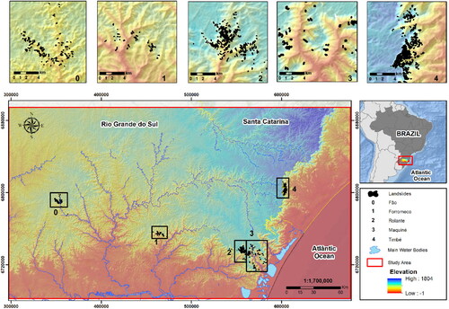
It consists predominantly of volcanic rocks, with an emphasis on basalts and andesites, and small portions of rhyolites and riodacites (Hartmann, 2014). It has structural lineaments in different directions, faulted relief, and soils with an average thickness of 50 centimeters (Betiollo, 2006).

The climate of the region varies depending on factors such as altitude and relief, according to Rossato (2011), it falls into humid subtropical with a longitudinal variation of average temperatures in the north-central region, and very humid subtropical with cold winter and cool summer in the region to the northeast, along the state border between Rio Grande do Sul and Santa Catarina. Summer is the most susceptible time for landslides in slope areas because it is when localized, intense, and short-term rainfall occurs.

2.2. Datasets

The data preparation relied primarily on the search for extreme events that occurred in the Serra Geral region, southern Brazil, and that had resulted in considerable landslides. An inventory of landslides was made and used as input to the modeling process.

SRTM images (spatial resolution: ∼90 m) were used to make a mosaic covering the entire length of the study area, and the terrain attributes created were used as landslide sample occurrence and non-occurrence values.

An ANN script, which contained the values of the morphometric attributes in each of the occurrence and non-occurrence samples, was used for the generation of landslide susceptibility models, which were analyzed through the Area Under the Receiver Operating Characteristic (ROC) Curve.

2.2.1. Landslide inventory

A reliable landslide inventory is vitally important for the analysis of LSM (Jebur et al. 2014). To formulate the landslide inventory, multi-temporal images from Google Earth Pro were used, for its accessibility and the spatial and temporal resolution of its images that facilitate the identification of landslides. The production of this inventory used the landslides of five sample areas in the Serra Geral (Table 1), all characterized as shallow landslides according to the classification of Highland and Bobrowsky (2008). In each sample area, a heavy precipitation event was recorded. Each heavy precipitation event triggered hundreds of landslides, all between 1995 and 2017.

Table 1. Location of landslide sample areas in Serra Geral, southern Brazil.

Sample Area	Hydrographic Basin	Counties	Precipitation Event (mm-yyyy)	Area Code
Fão River Valley	Taquari-Antas	Fontoura Xavier/Soledade	01-2010	0
Forromeco River Valley	Caí	São Vendelino/Carlos Barbosa	12-2000	1
Mascarada River Valley	Sinos	Rolante/São Francisco de Paula	01-2017	2
Maquiné River Valley	Maquiné	Maquiné	03-2007	3
Rocinha River Valley	Araranguá	Timbé do Sul/Jacinto Machado	12-1995	4

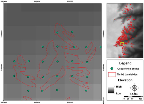
We mapped the landslide polygons using the Google Earth Pro multi-temporal imagery tool. After that, these polygons were transferred to the GIS environment and converted to points. We assign a point to each Digital Elevation Model (DEM) pixel that partially or fully intersects with landslide polygons. The spatial resolution of the DEM is 90 m, the same resolution used for the terrain attributes. In Figure 2, we exemplify the process of identifying the occurrence samples in a point feature, showing that the sampling points occur at the intersection between the landslide polygons and the SRTM pixels.

Figure 2. Example of converting polygons to point features to define the sample set of landslides occurrence.

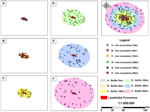
We used the 1:1 ratio for occurrence and non-occurrence samples. Bui et al. (2016) describe that LSM is a classic case of binary classification, in which the occurrence of a landslide results from the value 1, and the non-occurrence from the value 0. Following this logic, each point generated in the previous step was defined as a sample of occurrence, totaling 1638 points of occurrence, with 164 samples in area 0 (Fão), 60 in area 1 (Forromeco), 492 in area 2 (Rolante), 209 in area 3 (Maquiné), and 713 in area 4 (Timbé do Sul). Considering the non-occurrence samples, the respective number of points was generated for each area, resulting in 1638 points randomly distributed on the ground, with minimum distances of 150 m between them and with maximum distance limitations, attributed through the creation of buffers with distances of 2 km, 5 km, 10 km, 20 km, 30 km and 40 km of occurrence samples, as shown in Figure 3. That is, for each buffer used, 1638 random samples of non-occurrence were generated.

Figure 3. Example of buffer distances used for non-occurrence sampling.

2.2.2. Landslide conditioning factors

According to Jebur et al. (2014), there is no specific rule or structure for selecting and defining the importance of conditioning factors. Sixteen morphometric relief attributes were used (Figure 4), extracted using the Basic Terrain Analysis tool, in the SAGA GIS 7.0 software: elevation (ELV), slope (SLP), analytical hillshading (AHS), aspect (ASP), channel network base level (CNBL), vertical distance to channel network (VDCN), longitudinal curvature (LOC), cross-section curvature (CSC), flow accumulation (FAC), topographic wetness index (TWI), topographic position index (TPI), convergence index (CIN), relative slope position (RSP), mass balance index (MBI), valley depth (VDP) and LS factor (LSF). The definition of input variables was based on previous studies by Oliveira et al. (2019a), Quevedo et al. (2019), Lucchese et al. (2020) and Gameiro et al. (2021).

Figure 4. Terrain morphometric attributes used as input in the modeling.

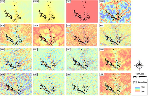
Attributes such as ELV, SLP, ASP and TWI are already widely used for landslide modeling (e.g. Jebur et al. 2014; Chen et al. 2017b; Hong et al. 2018b). The other attributes are also factors that can significantly influence the models since they are important relief features. These attributes, as well as the landslides, were generated through a digital elevation model with a resolution of 90 m, thus standardizing all the data used for modeling. Table 2 shows the basic descriptive statistics for each attribute, containing minimum, maximum, mean, and standard deviations.

Table 2. Statistical values of terrain morphometric attributes.

Attributes	Min	Mean	Max	Std dev.
ELV	−1.0	452.6	1804	355.7
SLP	0.0	5.9	62.5	6.7
AHS	0.0	0.8	2.1	0.2
ASP	0.0	179.3	360	99.7
CNBL	−1.0	398.5	1540	336.6
VDCN	0.0	54.1	880.7	77.6
LOC	−0.01	−0.00	0.04	0.0
CSC	−0.01	−0.00	0.01	0.0
FAC	7654	12577	25014	2300
TWI	3.5	9.6	27.0	3.8
TPI	−61.6	−1.8	47	2.3
CIN	−98.7	0.0	99.1	13.6
RSP	0.0	0.3	1	0.3
MBI	−0.67	0.05	2.16	0.15
VDP	0.0	113.2	755.1	99.6
LSF	0.0	1.8	133.4	2.7

Table 3 shows the mean and maximum areas of landslide polygons and the mean values of some of the most important morphometric attributes.

Table 3. Summary of landslides samples: mean and maximum areas of landslide polygons and the mean values of the some of the most important morphometric attributes.

	OCCURRENCE
	Mean Area (ha)	Máx Area (ha)	ELV	SLP	LSF	VDP
FÃO	0.22	1.0	477.35	22.10	9.10	184.55
FORROMECO	0.23	1.2	437.08	23.57	9.49	210.01
ROLANTE	0.34	4.0	590.13	26.52	11.49	307.93
MAQUINÉ	0.21	2.5	559.25	28.44	12.48	266.54
TIMBÉ DO SUL	0.56	6.1	692.26	30.27	11.87	248.91

After creating these attributes, many studies perform an analysis to find out how they relate to the model’s input variables (samples of occurrence and non-occurrence), using methods such as Pearson correlation (Bui et al. 2016; Wang et al. 2020; Lucchese et al. 2020). To hasten and improve the modeling process, Pearson correlation analysis was used to identify the attributes least correlated with the occurrence and non-occurrence samples and exclude them from the modeling process.

2.3. Modeling and validation

ANNs have been widely used for landslide modeling. Several studies reveal the usefulness and efficiency of these networks in LSM (Chen et al. 2017a; Kalantar et al. 2018; Oliveira et al. 2019a).

In the modeling process, an ANN script was used in the MATLAB software, with training carried out by the multilayer backpropagation method (Rumelhart; Hinton; Willians, 1986). To avoid overfitting the model, a series of cross-validation was used along with the training series. As in the studies of Oliveira et al. (2019a) and Lucchese et al. (2020), the proportion of samples is 50%/25%/25%, for training, cross-validation, and testing, respectively.

The training and cross-validation process was carried out in two steps. In the first step, in each round of modeling, samples were separated for each of the five sample areas and each of the six buffers (called Single Model). The ANN training considered each sample area and its buffers individually, generating a total of 30 datasets for modeling (5 areas × 6 buffers), showing how each sample area behaves when extrapolated to the entire region under study. In the next step, the samples from the five areas were used together in the modeling process (called Full Model), expanding the variability of the parameters. In this step, 6 datasets were generated for modeling, referring only to their respective buffers, showing the behavior of each one when used with samples of non-occurrence in different collection distances. In summary: i) Single Model uses as training samples only the landslides of one of the five areas, to measure the extrapolation capacity in the other four areas not used in the training; ii) Full Model uses as training samples a portion of the landslides of the five areas, to verify the performance increase when considering multiple precipitation events in different places of the study area.

For the initial configuration, the number of neurons in the hidden layer of the network followed the formula n-2, where n is the number of input variables used in the modeling. An automated increase in the number of neurons, up to a model with n + 6 neurons in the hidden layer, was tested; this was done to evaluate the increase in the models’ performance in relation to its greater complexity and synaptic weight. In each learning cycle, synaptic weight values are updated using the Delta Rule, based on the backpropagation of errors through the layers of the ANN. A maximum number of 10,000 learning cycles per iteration was established. Due to the random weight initialization, five iterations were performed in each model’s configuration.

In the validation process, accuracy was calculated using the ROC curve, which according to Jaafari et al. (2019) is the most popular scientific procedure for validating model prediction efficiency, being used for studies about floods (Hong et al. 2018b; Termeh et al. 2018) fires (Nami et al. 2018), and landslides (Chen et al. 2019; Oliveira et al. 2019a). The ROC curve is an analysis based on the final distribution of a classification method that differentiates correct and flawed forecasts (Cantarino et al. 2019), considered as the two-dimensional representation of a model’s performance.

In addition to the accuracy measured from the ROC curve, a confusion matrix was created to evaluate the performance of ANN models from the Global Accuracy (Equation (1)) and the Recall index (Equation (2)). The confusion matrix identifies the number of true positives (TP), false positives (FP), false negatives (FN), and true negatives (TN). TP shows the number of pixels correctly classified as susceptible, while FP are the pixels wrongly classified as susceptible. TN is the number of pixels correctly classified as not susceptible, and FN those incorrectly classified as not susceptible. (1) $$GlobalAccuracy=\frac{\left(TP+TN\right)}{(TP+TN+FP+FN)}$$(1) (2) $$Recall=\frac{TP}{(TP+FN)}$$(2)

Global Accuracy is one of the main performance metrics used in classification processes and shows the proportion of samples correctly classified in the LSM. Recall identifies what percentage are predicted positive from the total positive. It is the same as TPR (true positive rate). Hong et al. (2019b) and Bragagnolo et al. (2020), for example, used these metrics to evaluate their models.

The relative contribution index (RCI), proposed by Oliveira et al. (2015), was also used; it provides the importance values assigned by the ANN for each of the independent variables. RCI is obtained by imposing random perturbations on the values of input variables and measuring the effect caused on the output of the ANN. This index is calculated by dividing the contribution index (CI) by the sum of the CI over all model input, and it is a method for evaluating and defining more and less important variables according to each case.

3. Results

3.1. Landslide inventory and morphometry of sample areas

The mapping of landslide in the Serra Geral, in the south of Brazil, resulted in 1210 landslides, 121 in the Fão valley, 53 in the Forromeco valley, 338 in Rolante, 229 in Maquiné, and 469 in Timbé do Sul. When transformed into occurrence samples, 1638 samples were found. The same number of samples was generated to be used as non-occurrence samples, resulting in 3276 samples.

The most extreme precipitation events occurred in the regions of Timbé do Sul and Rolante, due to both the number of landslides and their size. In Timbé do Sul, the average area of landslides is 0.56 ha, and the largest reaches 6.1 ha. In Rolante, these values are 0.34 and 4.0 ha, respectively. Fão, Forromeco, and Maquiné obtained similar means, between 0.21 and 0.23 ha, noting only that in Maquiné the largest of the landslides has 2.5 ha, while in Fão and Forromeco it reached 1.0 and 1.2 ha, as shown in Table 3.

Besides the extreme events themselves, ELV and SLP values also influenced the quantity and dimensions of the landslides. When compared to Fão and Forromeco, the regions of Timbé, Maquiné, and Rolante, which have a greater amount and size of landslides, are also those that have a greater distinction in their ELV and SLP. In the first two, the ELV did not exceed 480 m, and the average slopes were 23.5°. In the other three, the ELV varied from 559 to 692 m, and the SLP was above 26.5°. This demonstrates that the morphometry of the relief is as closely linked to landslides as the intensity of the precipitation event that may have occurred.

Table 4 provides the averages of the attributes of each parameter for the best models generated with samples from only one sample area (best single model), and also with all sample areas (best full model). These values are extremely important because they demonstrate the great difference between the models based on the values used for training each one of them and also show the parameters with the greatest distinctions between each of the models.

Table 4. Attributes’ mean values in each of the best models for the occurrence samples.

	Best single model	Best full model
	Mean	Mean
SLP	22.10	25.87
AHS	1.13	1.16
CSC	−0.00	−0.00
LOC	−0.00	−0.00
LSF	9.18	10.71
TPI	−3.37	−2.55
TWI	7.31	6.99
VDP	184.55	246.79
VDCN	63.02	160.33
ELV	477.35	547.26
CIN	−4.25	−2.75
RSP	0.26	0.38
MBI	0.01	0.09

3.2. Correlation analysis and attribute selection

The attributes were analyzed using Pearson correlation (Table 5), with results ranging from −1 to 1. The closer to 0, the lower the correlation between the attribute and landslide occurrence, that is, the less influence it has on the landslide process. Thus, values between −0.8 and +0.8 were established as the threshold of choice between attributes, resulting in correlation values between −0.08 and +0.08 being excluded from the modeling process.

Table 5. Linear correlation coefficients for the independent variables with the model’s dependent variable (occurrence or non-occurrence of landslides) for each buffer. The values in red indicate the input variables that were excluded (in each dataset), due to the non-significant linear correlation.

	Buffers
	2 km	5 km	10 km	20 km	30 km	40 km	Mean
SLP	0.49	0.60	0.64	0.69	0.73	0.75	0.65
AHS	0.19	0.24	0.28	0.32	0.33	0.37	0.25
ASP	−0.04	−0.06	−0.07	−0.08	−0.06	−0.07	−0.06
CNBL	−0.16	−0.20	−0.17	−0.15	−0.10	−0.05	−0.14
CSC	−0.13	−0.15	−0.15	−0.18	−0.18	−0.17	−0.16
LOC	−0.22	−0.23	−0.23	−0.26	−0.24	−0.24	−0.23
LSF	0.49	0.60	0.64	0.70	0.73	0.74	0.65
TPI	−0.17	−0.18	−0.17	−0.21	−0.19	−0.19	−0.19
TWI	−0.14	−0.22	−0.28	−0.30	−0.36	−0.39	−0.28
VDP	0.25	0.30	0.32	0.38	0.36	0.36	0.33
VDCN	−0.09	0.09	0.19	0.27	0.38	0.42	0.21
ELV	−0.18	−0.14	−0.05	−0.01	0.07	0.14	−0.03
FAC	−0.02	−0.03	−0.04	−0.04	−0.05	−0.03	−0.04
CIN	−0.10	−0.10	−0.08	−0.11	−0.11	−0.10	−0.10
RSP	−0.24	−0.17	−0.08	−0.03	0.06	0.11	−0.06
MBI	−0.04	0.01	0.06	0.04	0.10	0.11	0.05

Among the 16 attributes generated, two stand out positively, with the highest correlation results for all buffers, and two stand out negatively, having practically no relation to landslides.

Attributes such as FAC, ASP and MBI were of no great value for the susceptibility analysis since they were not considered as correlated in most models, only MBI was used in models with distances of 30 and 40 km. ELV, an attribute used in practically all studies of LSM, showed variations according to the utilized buffers. This attribute proved to be effective when used for small areas (2 and 5 km) and large areas (40 km), but it was not effective when used over moderate distances. This is largely related to the great altimetric variability of some regions in the Serra Geral, even in small areas, which means that the amplitude of the non-occurrence values varies greatly in different regions.

3.3. Analysis and comparison of models

In Table 6, we present the values of Global Accuracy, Recall index, TP, FP, FN and TN for Full Model, considering all buffers. The same indices are presented in Table 7, considering the Single Model, with the best model trained from just one sample area.

Table 6. Performance metrics summary: Full Model, all buffers. Legend: TV = true positive; FP = false positive; FN = false negative; TN = true negative.

Full Model (Buffer)	TP (%)	FP (%)	FN (%)	TN (%)	Global Accuracy	Recall
2 km	36.69	13.31	8.36	41.64	0.783	0.814
5 km	39.26	10.74	5.40	44.60	0.838	0.879
10 km	41.61	8.39	4.43	45.57	0.871	0.903
20 km	43.35	6.65	3.54	46.46	0.898	0.924
30 km	43.47	6.53	1.71	48.29	0.917	0.962
40 km	44.84	5.16	1.43	48.57	0.934	0.968

Table 7. Performance metrics summary: only the best Single Model for each sample area. Legend: TV = true positive; FP = false positive; FN = false negative; TN = true negative.

Single Model (sample area and buffer)	TP (%)	FP (%)	FN (%)	TN (%)	Global Accuracy	Recall
Maquiné 30 km	42.98	6.93	4.80	45.29	0.882	0.899
Rolante 40 km	41.88	8.05	6.57	43.49	0.853	0.864
Forromeco 30 km	41.48	8.41	5.97	44.14	0.850	0.874
Fão 40 km	42.26	7.64	1.98	48.11	0.903	0.955
Timbé 40 km	46.17	3.83	3.56	46.44	0.926	0.928

It should be noted that the two best models were those with the lowest values of FN, which means that they were the models that had the lowest number of pixels incorrectly classified as not susceptible. This data is extremely relevant because it shows, through values, the number of susceptible pixels that the model classified as not susceptible.

In the best model with specific samples (Single Model), and which corresponds to the Fão 40 km model, the FN rate was 1.98%, that is, less than 2% of the pixels in the image were erroneously classified as not susceptible. However, the FP values were close to 8%, indicating that a significant amount of pixels were wrongly classified as susceptible, in areas with non-occurrence samples. The version of the Single Model configuration that presented the lowest FP value was Timbé 40 km. We emphasize that the global accuracy and the recall of the models with lower FN and FP were much higher than the other models, always reaching values above 0.90.

The same pattern was evidenced in the training rounds of the Full Model configuration. The models that used larger buffers to collect non-occurrence samples obtained lower FP and FN values. We observed that the errors made by the ANN model decrease as the distance of the non-occurrence samples increases in relation to the landslide polygons. For the best model with total samples (Full Model), these values were even lower, reaching 1.43% for FN and 5.16% for FP (Buffer 40 km).

For each model, five iterations were performed, so each buffer region generated five distinct models, totaling 30 for each sample area and 30 for the total area. With each new iteration, the model was initialized differently, thus generating different results. To standardize the models, the average accuracy of iterations was calculated, which resulted in a general accuracy for each model.

The influence of distance on the performance of the models is noticeable, both visually and statistically. In the analysis of the ROC curve, the average accuracy of the models (Table 8) of total samples ranged from 0.847 (Full Model 2 km) to 0.954 (Full Model 40 km), while, with the use of separate samples (Single Model), the values were between 0.872 (Timbé − 40 km) and 0.931 (Fão − 40 km). This highlights the quality of both techniques in the modeling process; however, it shows that better accuracy can be obtained when using a sample set with all areas combined, besides better differentiation and visual analysis, generating maps with less noise and more hits.

Table 8. Area under the ROC curve (Accuracy), considering test samples: Single and Full Models. In red the best models of the Single and Full version.

Buffer	Single model					Full model
	Maquiné	Rolante	Forromeco	Fão	Timbé	All Areas
2 km	0.788	0.759	0.813	0.810	0.791	0.847
5 km	0.879	0.817	0.868	0.861	0.848	0.902
10 km	0.912	0.739	0.874	0.896	0.871	0.932
20 km	0.916	0.824	0.874	0.897	0.861	0.947
30 km	0.926	0.786	0.919	0.919	0.872	0.942
40 km	0.912	0.873	0.907	0.931	0.872	0.954

Knowing the best model for each area, the quantification (in km²) of the regions with high susceptibility to landslides was performed (Table 9). Through this, it is noted that the models of Forromeco and Fão were very comprehensive, classifying as susceptible for 11,647 km² and 13,191 km² respectively. Meanwhile, the most restrictive model used Timbé samples, with 2,634 km² of susceptible area. The Maquiné, Rolante, and total sample models had intermediate susceptible areas, with results of 5324, 8968, and 5596 km², respectively.

Table 9. Area highly susceptible to landslides in each of the best models.

Best models	Single model					Full model
	Maquiné	Rolante	Forromeco	Fão	Timbé	All Areas
Area (km²)	5324	8968	11647	13191	2634	5596

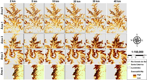
Figure 5 shows the best models for each buffer in the respective areas where the occurrence samples were extracted. There is better visual efficiency in the models with more distant buffers since they are more comprehensive in the subject of the values of utilized attributes, having a greater variation in these values and, consequently, facilitating the distinction between the susceptible areas by the ANN.

Figure 5. Comparison between models that used total samples (Full Model).

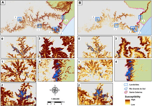
Figure 6 compares the two best models for each technique and highlights the five landslide areas used for sampling. The visual effect in each of the generated models is clearly perceived. The single model presents a noisier map regarding susceptibility, as it registers as susceptible regions with low or no presence of landslides. However, the full model shows a cleaner and more restrictive map if compared to samples from Fão. This is largely due to the values of the attributes used to make these models, as shown in Table 5.

Figure 6. Comparison of landslides areas between the best models: A) best model with separated samples, Single Model; B) best model with jointed samples, Full Model.

To analyze the similarities and differences between the two best models, a map algebra was applied to find the areas that stood out most in each of the models. The subtraction of the full model by the single model was applied (Figure 7). This map algebra resulted in a map with values between −1 and 1. The higher the value, the greater the susceptibility to landslides according to the full model. The lower the value, the greater the susceptibility according to the single model. If the results are close to 0, it means that the susceptibility of the two models was the same.

Figure 7. Subtraction between the best version of Full and Single Model.

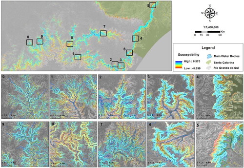
There were also 10 approaches to show the differences between the models, the five regions where landslide were found (0, 1, 2, 3, 4 – Fão, Forromeco, Rolante, Maquiné, and Timbé, respectively) and five regions without landslides (5, 6, 7, 8, 9), chosen to show the effectiveness of the models in different regions of Serra Geral.

The generated model presents a greater predominance of positive values, indicating that the full model reached higher values of susceptibility in different regions. The presence of positive values is widely highlighted, especially in the intermediate portions of Serra Geral, showing that those areas are highly susceptible to landslides. In areas of higher altitudes and low slopes (4, 5 and 6), such as the escarpment in Santa Catarina, and the bottoms of valleys and regions vertically closer to the drainage (2, 3, 4, 7 and 8), characterized by low altitudes and slopes, the single model showed higher susceptibility values.

3.4. Importance of morphometric attributes

Based on the ANNs, an assessment of the importance of attributes was made using the RCI calculation (Oliveira et al. 2019). Table 10 shows the values assigned to each attribute within the best model for each buffer.

Table 10. Relative Contribution Index (%) of each independent variable of the models.

Input variable	Buffers
	2 km	5 km	10 km	20 km	30 km	40 km
SLP	21	32	25	17	10	13
AHS	02	00	04	04	04	01
CNBL	14	13	19	13	21	–
CSC	04	06	06	02	06	00
LOC	01	01	01	02	01	01
LSF	04	02	02	05	07	02
TPI	02	03	04	07	03	03
TWI	05	02	04	03	02	01
VDP	08	03	08	08	07	06
VDCN	02	01	01	01	02	01
ELV	13	15	–	–	–	37
CIN	01	02	01	01	00	01
RSP	02	01	02	–	–	02
MBI	–	–	–	–	01	00

As Pearson correlation demonstrated, the SLP attribute is one of the main factors that influence LSM. However, there was a contrast between these values since, as the distance buffer increases, the SLP value increases in the Pearson correlation but decreases in the ANN analysis. CNBL also showed differences in the two analyzes, being highly valued by the ANN, mainly in the 30 km buffer, while in the correlation it presented median values that decreased as the distance increased.

To analyze the relation of importance between attributes and areas, 500 random points were generated within the 10 areas (0–9), plotted on a graph of the susceptibility of each of the best models and the main attributes found, using LSF, VDP, VDCN, SLP, and ELV (Figure 8).

Figure 8. Graphs showing the relation between the landslide susceptibility index from the best models and the main morphometric attributes.

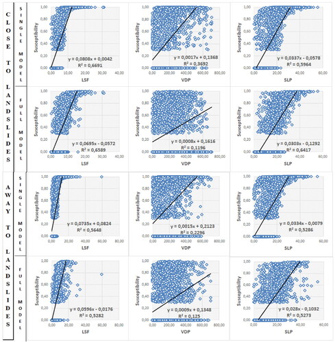
The graphs representing the susceptibility of the best models in relation to the main attributes show the relevance of these attributes on a linear scale and how representative they are in the modeling process. The LSF and SLP attributes stand out, with R² above 0.52, demonstrating a positive linear relationship with susceptibility, that is, susceptibility tends to increase as the values of these attributes also increase. This correspondence was repeated in both models and study areas; however, the highest LSF value (0.66) occurred in the single model, while the highest SLP value (0.64) occurred in the full model, both for areas close to landslides, thus reinforcing the idea that both attributes are important in landslide modeling.

Still on these two attributes, the LSF showed higher susceptibility to each increase in value, with an average susceptibility increase rate of 0.07 for each increase of the attribute. With the SLP, the increase rate was in the range of 0.03 for each degree of slope. Like the previous attributes, the VDP was also significant for modeling.

The VDCN and ELV attributes did not show significant relevance in their linear relationship with susceptibility. However, when ELV was analyzed individually, for each area and model, its importance is noticeable. Figure 9 shows the ELV analysis by model and collection area, with images A and B using points from all areas and C and D only using points from area 0. It is also emphasized that A and C refer to the single model and B and D refer to the full model.

Figure 9. Relationship between susceptibility index and elevation in the best models; A) Use of all samples for the single model; B) Use of all samples for the full model; C) Use of samples from area 0 for the single model; D) Use of samples from area 0 for the full model.

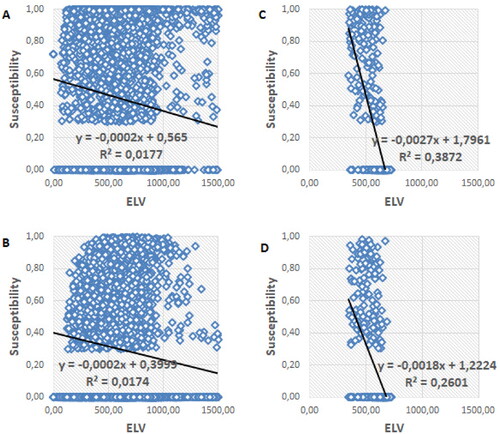
It is noticeable that even when considering the points of all areas together, the models did not show a significant linear relationship, with an R² of 0.01. This happens because the samples used for training are characterized by a wide range of values, making ELV undistinguished in the modeling process. When considering several landslide events, with spatially distant landslides and different precipitation rates for the occurrence of this type of mass movement, there is no pattern of typical altitude values for the breaking point and displacement of landslide materials.

4. Discussions

The attributes’ mean values are essential factors to understand the result of the model, as they explain the great difference between them according to the values used for training.

The SLP attribute for the Fão model has a mean value of 22°, while the total model obtained a mean value of 25°. This may explain why the Fão model has more susceptible areas in slope regions, as it considered smaller slopes as more susceptible to landslides, while the total model, with a higher mean value, restricted the model to map only regions with slopes of a 25 mean. Although slope angle is one of the most important factors for modeling susceptibility to landslides (Pradhan and Lee 2010), and, as stated by Meten et al. (2015), the greater the slope, the greater the susceptibility to material movement, care must be taken when analyzing its values. High slopes are not always an indication of an area susceptible to landslides.

LSF had the same behavior as SLP. This is because they are similar terrain attributes, and LSF calculation uses the slope angle value. For Quevedo et al. (2019), since SLP and LSF are highly correlated, having information in common, both tend to act in the same way in the modeling process, and, many times, when one of these factors is considered highly important, the other will have less relevance throughout the process.

Additionally, it is worth mentioning the VDP attribute, which also obtained higher mean values in the full model. Although it was only the fifth most important attribute on the ANN scale, for the total sample model, this attribute was the third most influential, only below SLP and ELV. It demonstrates that smaller valley depths also have significant importance in landslide processes.

ELV, as much as SLP, is one of the most effective attributes for this type of modeling (Kawabata and Bandibas 2009; Chen et al. 2017a). And, like SLP, ELV was vitally important for the creation of the models. The Fão model obtained lower means for this attribute, varying around 477 m, and classified as susceptible lower regions, the reverse of what occurred in the total model, which has elevations of 547 m. This variation is clear in the single model, where certain regions of the study area were widely classified as susceptible, even though they have characteristics such as moderate altitudes, low slopes, and large drainage networks.

The attributes with a higher correlation were SLP and LSF, with practically equal results in all analyzes and reaching an average correlation of 0.65, which is similar to the findings of Gameiro et al. (2019) and Lucchese et al. (2020). It should also be noted that the attributes AHS, CSC, LOC, TPI, TWI, VDP, VDCN and CIN were present in all modeling processes, as their correlation values were always above the pre-established limits, indicating that they are still attributes to consider in landslide susceptibility analyzes.

Besides, it is noteworthy that, although the distance influences the correct pixel values positively, the occurrence samples also influence the results. This is the case in Rolante, where even a 40 km buffer resulted in a model with high FN and FP due to the little representativeness that its occurrence samples have when compared with the other regions and with the entire Serra Geral area under analysis.

Moreover, a gradual increase in global accuracy and recall is noticeable as the collection distance of non-occurring samples increased, showing that the greater the collection distance is, the more representative the samples and the more accurate the generated models are. The full model obtained the highest values of these indexes, reaching 0.934 and 0.968, respectively. In the models with samples from each area, the single model was the one with the highest recall, obtaining 0.955; however, when analyzing global accuracy, the Timbé model was the one with the highest value.

The influence of distance on the performance of the models is noticeable, both visually and statistically. Despite that, the result with samples from Fão proved to be remarkably similar, statistically, with the results where all samples were used. Just like found by Polykretis et al. (2015), Oliveira et al. (2019a) and Gameiro et al. (2021), this indicates a good spatial extrapolation capacity of the ANN when the domains of the input values of the morphometric attributes are respected; that is, the extrapolation occurs efficiently in areas with more homogeneous geological and geomorphological characteristics.

It is worth mentioning that the best models used more distant samples of non-occurrence, as happened in studies by Oliveira et al. (2019b). This indicates that the more distant the buffer, the easier it will be for the ANN to discern between susceptible and non-susceptible areas, thus increasing the accuracy of the models.

Although Rolante is closer to the general mean among all models, the lack of representativeness of its samples meant that the model was not effective, both in terms of accuracy and space. It should also be noted that the model with total samples, which reached the highest accuracy, was restrictive, limiting the areas susceptible mainly to the upper half of the Serra Geral escarpments, where most of the landslides actually occur.

The best models for each buffer in the respective areas where the occurrence samples were extracted. It is noteworthy that those models with more distant buffers have less ‘noise’ in small areas close to the Serra Geral escarpment, are less restrictive, and show a greater degree of susceptibility in regions where there is a record of landslides.

The generated model presents a greater predominance of positive values, indicating that the full model reached higher values of susceptibility in different regions.

The reason for this great difference between the models’ results is mainly due to the samples used in training. Samples of occurrence in the single model, which used the Fão area, have lower slopes (22°), elevations (477 m), and vertical drainage distances (63 m), causing areas with these characteristics to be classified as more susceptible. Despite these small discrepancies, the remarkable capacity of ANN extrapolation when using only samples from a restricted area to model a wider region is emphasized.

In the full model, using training samples of greater amplitude and more representative of the entire Serra Geral, ANN managed to carry out a more efficient training, defining as susceptible areas already identified as susceptible to landslides.

This proves that the use of samples from different regions in the Serra Geral makes the modeling process more complex, since it uses occurrence data from different sample areas, thus increasing the differentiating power of ANN to model landslide susceptibility.

It should also be noted that the set of training samples needs to be representative of the entire region, with distinct attribute values between all the areas and units of relief present in its surroundings, thus increasing the effectiveness of the models.

The LSF attribute also greatly differed in the two analyzes. It obtained the highest values in the correlation, similar to the SLP, while for ANN it was of little relevance, contrasting to the results obtained by Oliveira et al. (2019). ELV, an attribute only used for 2, 5, and 40 km, according to the correlation analysis, was the most important attribute when used in the 40 km buffer. This corroborates the results of Youssef et al. (2016), Oliveira et al. (2019), and Quevedo et al. (2019), in which the ELV had more than 30% of importance. It demonstrates the importance of this attribute when using more varied samples of non-occurrence and that reach very different units of relief, greatly assisting ANN in distinguishing between susceptible and non-susceptible areas. The attributes MBI, RSP, CIN, and VDCN were shown to have the least influence by the network, obtaining values below 0.02. Despite that, the correlation between occurrences and VDCN proved to be of great value, especially for greater distances.

Despite obtaining lower values than SLP and LSF, it reached up to 0.36 value of linear ratio for the single model, demonstrating its importance and confirming the results of Oliveira et al. (2019), which found values of up to 24% for this attribute.

The geomorphological unit of Serra Geral presents a decline in altimetric values in the east-west direction, which causes the escarpment erosion line, and, consequently, the rupture points and material transport zones, to not present a preferential altitude for the occurrence of the phenomenon.

On the other hand, when only samples from Fão are used, with a well-defined interval of elevations, the linear relationship is present, showing that for small areas, training with simple samples (of only one area) makes the ELV a highly important attribute, reaching a mean R² = 0.32. However, it is not appropriate to use this small group of samples from a specific area to perform generalized extrapolations to large areas, mainly due to significant changes in the values of the morphometric attributes, because, when these attributes are not very representative, it ends up harming the performance of ANN (Nefeslioglu et al. 2008).

5. Conclusions

It is noticeable that the sample areas directly affect the result of landslide susceptibility modeling by ANN. The collection distance of non-occurrence samples is a determining factor for making highly accurate models, ensuing better results as this distance increases. The use of multiple events also showed great importance, generating better results due to the greater diversification of samples used for training. And it is also noted that there are morphometric attributes fundamental to the modeling process.

We conclude that the generalization and extrapolation capacity of ANN models allows their use in other contexts and areas of knowledge, involving the spatial dimension. We emphasize that this methodological approach of using samples from several events to model large areas, can also be suitable for other types of natural disasters, such as floods.

Among the main conclusions, the following stand out:

• The ELV and the SLP were the terrain attributes that most influenced landslide susceptibility. Depending on the sample set, the importance value of the two attributes can be reversed;

• The increase in the distance in the non-occurrence sampling process positively influences the accuracy of the models, going from 0.84 to 0.95 in total samples, and from 0.87 to 0.93 in samples from Fão;

• The process of choosing training samples is vitally important for the final result, and the choice of more diversified samples, collected in different areas, proved to have more efficient and accurate final results when compared to samples from specific regions and with similar morphometric characteristics;

• ANNs have a good capacity for spatial extrapolation, provided that the input value domains of the morphometric attributes are respected; in other words, if the extrapolation occurs to a homogeneous area in relation to landslide occurrences, a small area of evidence can obtain good results for larger and more distant areas.

Disclosure statement

No potential conflict of interest was reported by the authors.

Additional information

Funding

This research was supported by: i) CAPES (no. process 88882.438888/2011-01); ii) Fundação de Amparo à Pesquisa do Estado do Rio Grande do Sul (FAPERGS), Edital 01/2017 – ARD, no. process 17/2551-0000894-4; iii) Conselho Nacional de Desenvolvimento Científico e Tecnológico (CNPq), Chamada CNPq/MCTI/FNDCT N° 18/2021 – Faixa A – Grupos Emergentes, no. process 408489/2021-9.

References

- Aghdam IN, Varzandeh MHM, Pradhan B. 2016. Landslide susceptibility mapping using an ensemble statistical index (Wi) and adaptive neuro-fuzzy inference system (ANFIS) model at Alborz Mountains (Iran). Environ Earth Sci. 75(7):1–20.
- Baeza C, Lantada N, Moya J. 2010. Influence of sample and terrain unit on landslide susceptibility assessment at La Pobla de Lillet, Eastern Pyrenees, Spain. Environ Earth Sci. 60(1):155–167.
- Betiollo LM. 2006. Caracterização estrutural, hidrogeológica e hidroquímica dos sistemas aquíferos guarani e serra geral no nordeste do Rio Grande do Sul, Brasil. Dissertação (Mestrado em Geociências) – Instituto de Geociências, Universidade Federal do Rio Grande do Sul, p. 117.
- Blahut J, Van Westen CJ, Sterlacchini S. 2010. Analysis of landslide inventories for accurate prediction of debris-fow source areas. Geomorphology. 119(1-2):36–51.
- Bragagnolo L, da Silva RV, Grzybowski JMV. 2020. Artificial neural network ensembles applied to the mapping of landslide susceptibility. Catena. 184:104240.
- Bui DT, Tuan TA, Klempe H, Pradhan B, Revhaug I. 2016. Spatial prediction models for shallow landslide hazards: a comparative assessment of the efficacy of support vector machines, artificial neural networks, kernel logistic regression and logistic model tree. Landslides. 13(2):361–378.
- Cantarino I, Carrion MA, Goerlich F, Ibañez VMA. 2019. ROC analysis-based classification method for landslide susceptibility maps. Landslides. 16(2):265–282.
- Chen W, Pourghasemi HR, Kornejady A, Zhang N. 2017a. Landslide spatial modeling: introducing new ensembles of ANN, MaxEnt, and SVM machine learning techniques. Geoderma. 305:314–327.
- Chen W, Pourghasemi HR, Panahi M, Kornejady A, Wang J, Xie X, Cao S. 2017b. Spatial prediction of landslide susceptibility using an adaptive neuro-fuzzy inference system combined with frequency ratio, generalized additive model, and support vector machine techniques. Geomorphology. 297:69–85.
- Chen W, Panahi M, Tsangaratos P, Shahabi H, Ilia I, Panahi S, Li S, Jaafari A, Ahmad BB. 2019. Applying population-based evolutionary algorithms and a neuro-fuzzy system for modeling landslide susceptibility. Catena. 172:212–231.
- Di Napoli M, Carotenuto F, Cevasco A, Confuorto P, Di Martire D, Firpo M, Pepe G, Raso E, Calcaterra D. 2020. Machine learning ensemble modelling as a tool to improve landslide susceptibility mapping reliability. Landslides. 17(8):1897–1914.
- Dornik A, Drăguţ L, Oguchi T, Hayakawa Y, Micu M. 2022. Influence of sampling design on landslide susceptibility modeling in lithologically heterogeneous areas. Sci Rep. 12(1):2106. |
- Gameiro S, Quevedo RP, Oliveira GG, Ruiz LFC, Guasselli LA. 2019. Análise e correlação de atributos morfométricos e sua influência nos deslizamentos ocorridos na Bacia do Rio Rolante, RS. In Simpósio Brasileiro de Sensoriamento Remoto, XIX, Santos. Anais... Santos, Vol 17, p. 2880–2883.
- Gameiro S, Riffel ES, Oliveira GG, Guasselli LA. 2021. Artificial neural networks applied to landslide susceptibility: the effect of sampling areas on model capacity for generalization and extrapolation. Appl Geogr. 137:102598.
- Görum T. 2019. Landslide recognition and mapping in a mixed forest environment from airborne LiDAR data. Eng Geol. 258:105155.
- Hartmann LA. 2014. A história natural do Grupo Serra Geral desde o Cretáceo até o Recente. Ciência E Natura. 36(3):173–182.
- Heckmann T, Gegg K, Gegg A, Becht M. 2014. Sample size matters: investigating the effect of sample size on a logistic regression susceptibility model for debris flow. Nat Hazards Earth Syst Sci. 14(2):259–278.
- Highland LM, Bobrowsky P. 2008. The landslide handbook - a guide to understanding landslides: Reston, Virginia, U.S. Geological Survey Circular 1325:129.
- Hong H, Pradhan B, Xu C, Bui DT. 2015. Spatial Prediction of landslide hazard at the Yihuang area (China) using two-class kernel logistic regression, alternating decision tree and support vector machines. Catena. 133:266–281.
- Hong H, Tsangaratos P, Ilia I, Liu J, Zhu A-X, Chen W. 2018a. Application of fuzzy weight of evidence and data mining techniques in construction of flood susceptibility map of Poyang County, China. Sci Total Environ. 625:575–588.
- Hong H, Liu J, Bui DT, Pradhan B, Acharya TD, Pham BT, Zhu A-X, Chen W, Ahmad BB. 2018b. Landslide susceptibility mapping using J48 Decision Tree with AdaBoost, Bagging and Rotation Forest ensembles in the Guangchang area (China). Catena. 163:399–413.
- Hong H, Miao Y, Liu J, Zhu A-X. 2019a. Exploring the effects of the design and quantity of absence data on the performance of random forest-based landslides susceptibility mapping. Catena. 176:45064.
- Hong H, Shahabi H, Shirzadi A, Chen W, Chapi K, Ahmad BB, Roodposhti MS, Hesar AY, Tian Y, Bui DT. 2019b. Landslides susceptibility assessment at the Wuning area, China: a comparison between multi-criteria decision making, bivariate statistical and machine learning methods. Nat Hazards. 96(1):173–212.
- Jaafari A, Panahi M, Pham BT, Shahabi H, Bui DT, Rezaie F, Lee S. 2019. Meta optimization of an adaptive neuro-fuzzy inference system with grey Wolf optimizer and biogeography-based optimization algorithms for spatial prediction of landslide susceptibility. Catena. 175:430–445.
- Jebur MN, Pradhan B, Tehrany MS. 2014. Optimization of landslide conditioning factors using very high-resolution airborne laser scanning (LiDAR) data at catchment scale. Remote Sens Environ. 152:150–165.
- Jennifer JJ, Saravanan S. 2021. Artificial neural network and sensitivity analysis in the landslide susceptibility mapping of Idukki district, India. Geocarto Int. 37(19):5693–5715.
- Kalantar B, Pradhan B, Naghibi SA, Motevalli A, Mansor S. 2018. Assessment of the effects of training data selection on the landslide susceptibility mapping: a comparison between support vector machine (SVM), logistic regression (LR) and artificial neural networks (ANN). Geomatics Nat Hazards Risk. 9(1):49–69.
- Kawabata D, Bandibas J. 2009. Landslide susceptibility mapping using geological data, a DEM from ASTER images and an Artificial Neural Network (ANN). Geomorphology. 113(1-2):97–109.
- Khanna K, Martha TR, Roy P, Kumar KV. 2021. Effect of time and space partitioning strategies of samples on regional landslide susceptibility modelling. Landslides, Technical Note. 18(6):2281–2294.
- Lucchese LV, Oliveira GG, Pedrollo OC. 2020. Attribute selection using correlations and principal components for artificial neural networks employment for landslide susceptibility assessment. Environ Monit Assess. 192(2):129.
- Meten M, Prakashbhandary N, Yatabe R. 2015. Effect of landslide factor combinations on the prediction accuracy of landslide susceptibility maps in the Blue Nile Gorge of Central Ethiopia. Geoenviron Disasters. 2(1):1–17.
- Nami MH, Jaafari A, Fallah M, Nabiuni S. 2018. Spatial prediction of wildfire probability in the Hyrcanian ecoregion using evidential belief function model and GIS. Int J Environ Sci Technol. 15(2):373–384.
- Nefeslioglu HA, Duman TY, Durmaz S 2008. Landslide susceptibility mapping for a part of tectonic Kelkit Valley (Eastern Black Sea region of Turkey). Geomorphology. 94(3–4):401–418.
- Novellino A, Cesarano M, Cappelletti P, Di Martire D, Di Napoli M, Ramondini M, Sowter A, Calcaterra D. 2021. Slow-moving landslide risk assessment combining Machine Learning and InSAR techniques. Catena. 203:105317.
- Oliveira GG, Pedrollo OC, Castro NMR. 2015. Simplifying artificial neural network models of river basin behaviour by an automated procedure for input variable selection. Eng Appl Artif Intell. 40:47–61.
- Oliveira GG, Ruiz LFC, Guasselli LA, Haetinger C. 2019a. Random Forest and artificial neural networks in landslide susceptibility modeling: a case study of the Fão River Basin, Southern Brazil. Nat Hazards. 99(2):1049–1073.
- Oliveira GG, Ruiz LFC, Quevedo DM. 2019b. Redes neurais artificiais e geotecnologias para o mapeamento de áreas suscetíveis a inundações. In: Simpósio Brasileiro de Recursos Hídricos, XXIII, 2019 Foz do Iguaçu. Anais XXIII Simpósio Brasileiro de Recursos Hídricos. Porto Alegre: ABRH, 2019. Vol1. p. 1–10.
- Pandey VK, Sharma MC. 2017. Probabilistic landslide susceptibility mapping along Tipri to Ghuttu highway corridor, Garhwal Himalaya (India). Remote Sens Appl Soc Environ. 8:1–11.
- Petschko H, Bell R, Brenning A, Glade T. 2012. Landslide susceptibility modeling with generalized additive models–facing the heterogeneity of large regions. Landslides Eng Slopes Protect Soc Improv Underst. 1:769–777.
- Petschko H, Brenning A, Bell R, Goetz J, Glade T. 2014. Assessing the quality of landslide susceptibility maps – case study Lower Austria. Nat Hazards Earth Syst Sci. 14(1):95–118. 2014.
- Polykretis C, Ferentinou M, Chalkias C. 2015. A comparative study of landslide susceptibility mapping using landslide susceptibility index and artificial neural networks in the Krios River and Krathis River catchments (northern Peloponnesus, Greece). Bull Eng Geol Environ. 74(1):27–45.
- Pourghasemi HR, Pradhan B, Gokceoglu C. 2012. Application of fuzzy logic and analytical hierarchy process (AHP) to landslide susceptibility mapping at Haraz watershed, Iran. Nat Hazards. 63(2):965–996.
- Pradhan B, Lee S. 2010. Regional landslide susceptibility analysis using backpropagation neural network model at Cameron Highland, Malaysia. Landslides. 7(1):13–30.
- Quevedo RP, Guasseli LA, Oliveira GG, Ruiz LFC. 2019. Modelagem de áreas suscetíveis a deslizamentos: avaliação comparativa de técnicas de amostragem, aprendizado de máquina e modelos digitais de elevação. São Paulo, UNESP, Geociências. 38(3):781–795.
- Regmi AD, Devkot KC, Yoshida K, Pradhan B, Pourghasemi HR, Kumamoto T, Akgun A. 2014. Application of frequency ratio, statistical index, and weights-of-evidence models and their comparison in landslide susceptibility mapping in Central Nepal Himalaya. Arab J Geosci. 7(2):725–742.
- Rossato MS. 2011Os climas do Rio Grande do Sul: variabilidade, tendências e tipologia. Tese (Doutorado), Instituto de Geociências, Programa de Pós-Graduação em Geografia da Universidade Federal do Rio Grande do Sul, p. 253.
- Sachdeva S, Bhatia T, Verma AK. 2020. A novel voting ensemble model for spatial prediction of Landslides using GIS. Int J Remote Sens. 41(3):929–952.
- Sameen MI, Pradhan B, Lee S. 2020. Application of convolutional neural networks featuring Bayesian optimization for landslide susceptibility assessment. Catena. 186:104249.
- Shirzadi A, Solaimani K, Roshan MH, Kavian A, Chapi K, Shahabi H, Keesstra S, Ahmad BB, Bui DT. 2019. Uncertainties of prediction accuracy in shallow landslide modeling: Sample size and raster resolution. Catena. 178:172–188.
- Termeh SVR, Kornejady A, Pourghasemi HR, Keesstra S. 2018. Flood susceptibility mapping using novel ensembles of adaptive neuro fuzzy inference system and metaheuristic algorithms. Sci Total Environ. 615:438–451.
- Valenzuela P, Domínguez-Cuesta MJ, García MAM, Jiménez-Sánchez M. 2017. A spatio-temporal landslide inventory for the NW of Spain: BAPA database. Geomorphology. 293:11–23.
- Van Den Eeckhaut M, Hervás J, Jaedicke C, Malet J-P, Montanarella L, Nadim F. 2012. Statistical modelling of Europe-wide landslide susceptibility using limited landslide inventory data. Landslides. 9(3):357–369.
- Xiong Y, Zhou Y, Wang F, Wang S, Wang Z, Ji J, Wang J, Zou W, You D, Qin Q. 2022. A novel Intelligente method based on the gaussian heatmap sampling technique and convolutional neural network for landslide susceptibility mapping. Remote Sens. 14(12):2866.
- Yalcin A. 2008. GIS-based landslide susceptibility mapping using analytical hierarchy process and bivariate statistics in Ardesen (Turkey): comparisons of results and confirmations. Catena. 72(1):1–12.
- Yilmaz I. 2009. Landslide susceptibility mapping using frequency ratio, logistic regression, artificial neural networks and their comparison: a case study from Kat landslides (Tokat – Turkey). Comput Geosci. 35(6):1125–1138.
- Youssef AM, Pourghasemi HR, Pourtaghi ZS, Al-Katheeri MM. 2016. Landslide susceptibility mapping using random forest, boosted regression tree, classification and regression tree, and general linear models and comparison of their performance at Wadi Tayyah Basin, Asir Region, Saudi Arabia. Landslides. 13(5):839–856.
- Zhao F, Meng X, Zhang Y, Chen G, Su X, Yue D. 2019. Landslide susceptibility mapping of Karakorum Highway combined with the application of SBAS-InSAR technology. Sensors. 19:2685
- Zhu A-X, Miao Y, Yang L, Bai S, Liu J, Hong H. 2018. Comparison of the presence-only method and presence-absence method in landslide susceptibility mapping. Catena. 171:222–233.
- Zhu A-X, Miao Y, Liu J, Bai S, Zeng C, Ma T, Hong H. 2019. A similarity-based approach to sampling absence data for landslide susceptibility mapping using data-drive methods. Catena. 183:104188.
- Wang Y, Fang Z, Hong H. 2019. Comparison of convolutional neural networks for landslide susceptibility mapping in Yanshan County, China. Sci Total Environ. 666:975–993.
- Wang Y, Feng L, Li S, Ren F, Du Q. 2020. A hybrid model considering spatial heterogeneity for landslide susceptibility mapping in Zhejiang Province, China. Catena. 188:104425.