Land cover classification using Land Parcel Identification System (LPIS) data and open source Eo-Learn library

Abstract

Depending on the development of remote sensing technologies, data at various spatial, temporal and spectral resolutions are obtained and play a key role in Earth investigation. Land cover/use maps are also created using these data. These data play an important role as a base for determining land cover and land use classes, detecting changes, monitoring forest, agriculture and wetlands, as well as updating the LPIS data used by countries. As well as being reference data in the LPIS update, current land cover and land use classification results with satellite images also provide statistical information about which class has changed over the years and how much the class or classes need to be updated, and will also provide the planning of the update to be made on a national scale. In this study, land cover classification for 2020 covering Çivril-Baklan Plain, which is between the borders of Denizli Province (Turkey), Baklan, Çal and Çivril Districts, was performed. The LPIS classes of the study area drawn in 2015 and the land cover classes as a result of the 2020 classification were compared as a result of the classification process, and particularly the areas with change were referenced in the LPIS update. In the classification process, the open source Eo-Learn library, which uses machine learning and deep learning algorithms in remote sensing studies and Sentinel-2 images that can be accessed directly in this library were used. The open source Eo-Learn library has been preferred because it provides great convenience to users in the classification process with ready-made machine learning models and easy access to satellite images, image processing steps (cloud masking, calculate index, feature extraction, temporal interpolation) are carried out in a certain workflow. Instead of land cover classification from a single image, 17 different time (multi-temporal) images between 01.02.2020 and 31.11.2020 were used. In the classification process, 12 different features were used for the image taken on each date, including NDVI, NDWI, NDBI indices and Tasseled Cap transformations, as well as (Blue) B02, (Green) B03, (Red) B04, (NIR) B08, (SWIR-1) B11, (SWIR-2) B12 bands. In the classification process, the Light Gradient Boosting Machines (LightGBM) algorithm in the Eo-Learn library and the physical blocks produced within the scope of the Land Parcel Identification System (LPIS) project were used as ground truth data; arable land, bare land, forest, artificial surface, shrubland, tree crops and water classes were created. The classification results were evaluated using the K fold (k = 5) cross validation method, with F1 score, recall, and precision values calculated for each class, and the overall accuracy %92.2. When the classification result is compared with the LPIS data, it is seen that the arable land, shrub land, and water classes have changed. This study determined that these classes, in particular, need to be updated.

Keywords:

• Eo-Learn
• Sentinel-2
• IACS
• LPIS
• classification
• machine learning
• remote sensing
• land cover

1. Introduction

Land cover mapping plays a key role in providing critical information for many applications such as urban planning, agricultural activity environmental management and natural resource management. In particular, the wide availability of multi temporal satellite images, as well as the advancement in digital image processing, enabled the monitoring, assessment and understanding of spatial and temporal variation in land cover. Multi-temporal images play an important role in monitoring dynamic changes in land cover (especially in agricultural areas). The choice of classification algorithms should also be taken into consideration since time series data are more complex than single-date data (Candido et al. 2021).

As the spectral, temporal and spatial resolution of satellites increases and in case being wide study area manual identification, downloading, of multi-time images going through various image processing steps and performing classification takes a lot of time and becoming complicated. With the advancement of technology, numerous remote sensing libraries and platforms can help with these and similar situations. One of them is the Eo-Learn library. Eo-learn is an open source package for data science and machine learning (ML) that integrates an automatic pipeline for downloading, preprocessing and processing the different types of satellite images (Peressutti 2018). Eo-Learn library to automate and parallelize the different tasks of large amounts of data, a processing flow has been created by the Eo-learn tasks (Jarray et al. 2021). The library is divided into several subpackages according to different functionalities and package dependencies. The library is written in python and uses numpy arrays to store and handle remote sensing data. It aims to make entry easier for non-experts to the field of remote sensing on one hand and bring the state-of-the-art tools for computer vision, machine learning and deep learning existing in the python ecosystem to remote sensing experts (https://eo-learn.readthedocs.io/en/latest/). In summary, Eo-learn library acts as a bridge between earth observation - remote sensing field and python ecosystem for data science and machine learning.

The land cover classification was made by deep learning at the whole Slovenia scale using the Eo-Learn library. In this classification process, land cover classification was performed using multi-time Sentinel-2 images at 10-day intervals rather than a single image, and the classification success rate was % 95.6 (Lubej et al. 2019). 13 agricultural products were classified using the parcels obtained from the Slovenian Agricultural Markets and Rural Development Agency and the Eo-Learn library. As a result of the classification, the success rate was %72 with the LightGBM algorithm, while this rate increased to %87 with deep learning (Račič et al. 2020).

Soil moisture estimation was carried out in an area of approximately 140 km2 in Medenine, Tunisia, using the Eo-Learn library and Sentinel-1 and Sentinel-2 images. As a result of the study %, 88 success was achieved with the random forest algorithm, %79 with the XGboost algorithm, and %76 with the artificial neural networks (Jarray et al. 2021).

Image processing can take a lot of time in classification processes with multi-temporal images using a large number of ground truth data. Determining and downloading the images to be used, separating the cloudy images or identifying and masking the cloudy areas, creating features and indices from the images, combining all the created layers, particularly if it is done manually takes time, and is not sustainable. The open source Eo-Learn library can provide access to various satellite images, and images can be obtained by specifying the start and end dates, as well as the desired image shooting frequency. Identifying and masking cloudy areas with the help of subpackages in the library, image co-registration, feature extraction, calculate index, merging all the created layer, determining the optimum parameters of the model to be used in the classification process, the automatic separation of the created model into training and test data with the k-fold cross validation method, the classification process and the determination of the error matrix and accuracy values are made within a certain workflow framework, providing a great convenience for the users, especially in large areas.

In this study, land cover classification for 2020 was performed using the open source code Eo-Learn library in the study area covering the Çivril-Baklan Plain of Denizli Province. The result of the land cover classification (2020) and the physical blocks (2015) at LPIS classes were compared and the areas that needed updating were identified. This study is also a demo of a larger study that will be conducted on a national scale.

2. Study area and datasets

2.1. Study area

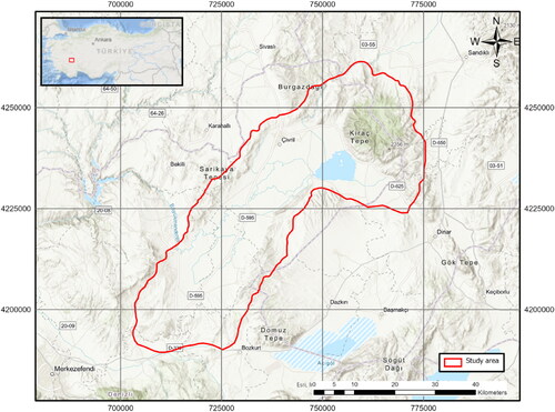
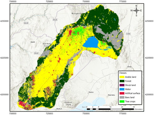
The study area is within the boundaries of Denizli Province Çivril, Baklan and Çal Districts, with an average height of 1000 m and a width of 3500 km2 and covers the entire Çivril-Baklan Plain (Figure 1). Çivril and Baklan Plain has a transition type climate between the Mediterranean climate seen in the Aegean Region and the continental climate seen in Central Anatolia. The summers are hot and dry, while the winters are cold and rainy. Büyük Menderes, the most important river of the Aegean region, passes through and irrigates the Çivril-Baklan Plain, which is a semi-closed basin (Aksever and Eroğlu 2016). Işıklı Lake is located on the Büyük Menderes Stream, and it provides agricultural irrigation to the plain, allowing various agricultural products to be grown. Akdağ, the highest mountain in the region, is located in the north of the study area. It has been determined as an ideal study area as it includes various land cover usage classes and particularly agricultural areas and wetlands, which show variability throughout the year.

Figure 1. Study area; Denizli – Çivril Province, Turkey.

2.2. Land Parcel Identification System

The Integration Administration Control System (IACS) is a system that provides the management and administration of agricultural supports (Lüker-Jans et al. 2016). In the European Union’s member states, IACS is used in the calculation and control of payments for the correct and timely payment of direct payments distributed to farmers (Harvolk et al. 2014). LPIS is an integral part of Common Agricultural Policy’s Integration Administration Control System (IACS) (Efthimiou et al. 2022). LPIS is a subcomponent of IACS. LPIS is the GIS that allows IACS to geolocate, display and spatially integrate its many data. It thus contains many spatial data sets from multiple sources and of different nature. To support the appropriate level of compatibility between these, it is necessary to describe some basic properties of these spatial data sets and how they behave in framework of the IACS (Luketic et al. 2015). LPIS spatially represent the activities of farmers and their land, based on Geographic Information Systems (GIS), allowing area-based payments for geographic location and extent/type of the agricultural activity (Inan et al. 2010).

The Turkish Ministry of Agriculture and Forestry’s General Directorate of Agricultural Reform developed the Land Parcel Identification System as part of the IACS project, using 1/5000 scale aerial photographs and satellite images, as well as geographic information systems and digitizing reference parcels. In setting up a Land Parcel Information System in Turkey an initial decision was made on the type of reference parcel to be adopted. Across Europe a range of different approaches have been utilised, based either on the agricultural parcel, the farmer’s block, the cadastral parcel or the physical block (Figure 2). These definitions are based on photo interpretation and digitization guidelines for Turkey.

Figure 2. Physical block definition.

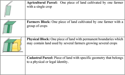
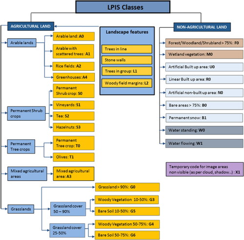
In Turkey, because of the size of the country and the nature of the agricultural landscape, the physical block has been chosen as the Reference Parcel to be used. A physical block is a ‘production block’, delineated by the national administration (not farmers), and based, as far as possible, on visible and relatively permanent boundary phenomena. The production block is a unit of (spatially continuous) agricultural activity, either related to production or to a minimum level of maintenance. In this respect, the physical block represents the smallest identifiable true unit of agricultural practice. It can be called also ‘unit of land management’. In this study, LPIS classes (physics blocks) were used as reference data in land cover classification (Figure 3).

Figure 3. Land parcel identification system (LPIS) classes in Turkey.

2.3. Eo-Learn library

Eo-Learn is an open source python library that uses machine learning and deep learning algorithms in data science, earth observation and remote sensing studies (Lubej 2018). Given the large amount of data at high revisit frequency, Eo-Learn requires frameworks capable of automatically extracting complex patterns data. It aims at providing a set of tools to make prototyping of complex EO workflows as easy, fast, and accessible as possible (Peressutti 2018).

Eo-Learn provides access to many satellite images such as Landsat, Sentinel, Modis, Envisat etc. With Eo-Learn, complex remote sensing studies such as automatic cloud detection and masking, land cover classification, crop classification, object based classification, automatic parcel boundary delineation, feature extraction, super pixel on satellite images can be performed using machine learning and deep learning methods with ready-made pipeline models to store and process remote sensing data, the Eo-Learn library employs the numpy library, a basic python library for scientific computations that handles multidimensional arrays and matrices. In addition the main libraries it uses are; gdal, rasterio, shapely, fiona, cartopy and pyproj libraries (https://github.com/sentinel-hub/eo-learn). The Eo-Learn library is divided into sub-packages according to different functions and it also provides the user with the opportunity to install one or more of the sub-packages according to the process the user needs instead of installing the whole library.

One important aspect of pipelines is that they divide the working area into smaller chunks and for each one created an EO-Patch, which stores all the data from that location. These operations are performed on the local computer. EOPatch instances are performed by EOTask instances. Tasks are grouped by scope and packaged into separate python sub-packages, which are; eo-learn-core, eo-learn-io, eo-learn-mask, eo-learn-features, eo-learn-ml-tools, eo-learn-coregistration. In this study, Light GBM algorithm in eo-learn-ml-tools, which is one of its sub-packages for Eo-learn library, was used for land cover classification.

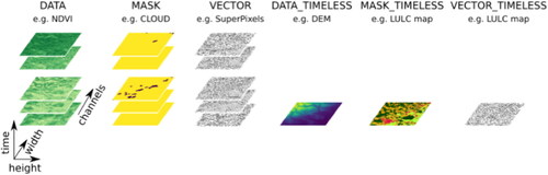
The pipeline can run operations on multiple EO-Patches in parallel while keeping only as much data in memory as the available resources. This makes the execution part of the pipeline much faster and more convenient (Aleksandrov and Visnjic 2020). An EO-Patch instance is uniquely defined by the coordinates of a bounding box and the time-interval the stored data refers to (Figure 4). Information in any format readable by Python packages can also be stored in EO-Patch objects

Figure 4. Structure of an EO-Patch (from https://medium.com/sentinel-hub/introducing-eo-learn-ab37f2869f5c).

3. Methodology

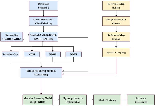
Sentinel-2 images were used as satellite images in the study. Sentinel-2 is launched by the European Space Agency (ESA) within the scope of the European Union’s Copernicus Environmental Monitoring Program, has 13 spectral bands with a taking frequency of 5 days and different spatial resolutions (10 m, 20 m, 60 m), a fleet of earth observation satellites with active sensors. Sentinel-2 images contain 13 spectral bands and have a temporal resolution of 5 days. It supports a wide range of services and applications such as monitoring of agricultural areas, land cover classification, emergency management and monitoring of water resources. A flowchart showing land cover classification with Eo-Learn library and Sentinel-2 images is shown below (Figure 5). The method consists of 3 steps; data pre-processing and feature sets, reference data preparation, machine learning and classification.

Figure 5. Flowchart of the study.

3.1. Satellite data pre-processing and feature sets

Sentinel-2 images are accessed using the sentinelhub py python package within the open EoLearn library (https://sentinelhub-py.readthedocs.io/en/latest/configure.html#sentinel-hub-configuration). With this package, satellite images stored in Amazon Cloud are provided by connecting to Sentinel-Hub (https://github.com/sentinel-hub/sentinelhub-py/). Sentinel Hub is a simple and efficient way of archiving, processing and distributing satellite data using standard web services that can be easily integrated into any desktop, web or mobile mapping application. All information of satellite images (bands, forming indexes, cloud masks, etc.) is stored in each EO-Patch as a time series integrated with numpy sequences, and information that can be read in any format by python packages can also be stored in EO-Patchs.

In the study, land use classification was not carried out from a single satellite image. Since especially agricultural areas and shrub land areas vary throughout the year, time series images are provided. Land use classification with multi-time images gives higher accuracy compared to a single image (Zheng et al. 2017). It has been determined that the use of spectral vegetation indices such as NDVI, especially in the form of time series (Foerster et al. 2012) easily distinguishes agricultural areas from similar classes in classification and gives high scores (Viana et al. 2019).

Although the study area contains a large agricultural area, it also contains a wetland that meets the water needs of these agricultural areas. Cultivated areas and fruit trees change throughout the year as a result of agricultural activities (on satellite images), and the wetland changes as a result of both meteorological conditions and agricultural irrigation. Detecting the areas of these classes, which change throughout the year, on a single image may mislead us. For this reason, it is aimed to determine these classes correctly and to increase the accuracy of classification by using more images, bands and indexes. Thus, 17 images in the form of a time series spanning a year and indices created from images were used in the classification process.

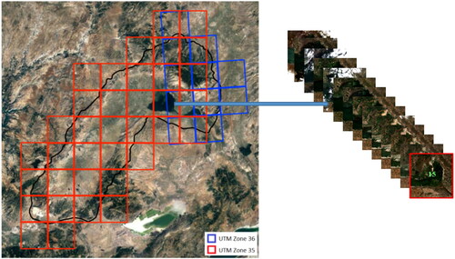
With the Eo-Learn library, parameters such as start date, end date and image acquisition interval were determined and provided by dividing them into segments (EO-Patch) as an integrated time series. In this study, Sentinel-2 L1C images were obtained between 01.02.2020 − 31.11.2020 by dividing into 10*10 km partitions (EO-Patch) with 15-day intervals. If more than 30% of the area of the images provided is covered with cloud, it is automatically excluded from the process with the Sen2cloudless python library, and this threshold value can be changed (Figure 6).

Figure 6. The area-of-interest split into smaller patches 1000 x 1000 square pixels at 10 m resolution.

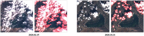
Clouds arising from atmospheric effects, and shadows from clouds in satellite images are the main sources of noise that cause problems in the analysis of images. (Kalkan and Maktav 2016). The brightness caused by the clouds and shadows affect the data analysis negatively. These effects cause the values of NDVI etc. indexes to change, and errors to occur in various analyzes and classification processes (Zhu and Woodcock 2012). With the Sen2cloudless package in the Eo-Learn library, the clouds on the satellite image are automatically detected and masked (Zupanc 2017). Sen2cloudless cloud detection and masking package works by using LightGBM algorithm with the pixel-based Sentinel-2 satellite B01, B02, B03 B04, B05, B08, B8A, B09, B10, B11, B12 bands (Figure 7).

Figure 7. Cloud detection and masking with Sen2cloudless.

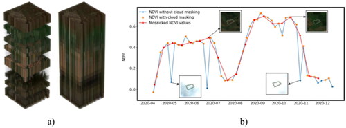
Cloud-covered areas cause anomalies in the bands in the images as well as the pixel values in the indexes created from these bands, which may adversely affect the classification result (Karlsen et al. 2021). In order to eliminate this situation, after the detection and masking of the cloudy areas, the bands with anomalies and the pixel values in the indices produced from these bands are temporal interpolated with reference to the pixel and band values in the image before and after them (Figure 8).

Figure 8. Temporal stack with missing data due to clouds before temporal interpolation left and after right (a).(https://medium.com/sentinel-hub/land-cover-classification-with-eo-learn-part-2-bd9aa86f8500) Cloud detection, masking and comparison of the original unmasked and masked NDVI profile of a meadow in parcel (b).

In the study, with 10 meters spatial resolution blue (B02), green (B03), red (B04) and near infrared (B08) bands and short-wave infrared-1 (SWIR-1) and short-wave infrared-2 (SWIR-2) bands which were resampled from 20 meters spatial resolution to 10 meters spatial resolution were used. Additional data is used to increase the accuracy of classification, or in other words, to increase the distinguishability of land use or crop pattern classes from each other (Üstüner et al. 2015). Classification accuracy also depends on the appropriate spectral band and indices produced from these bands, depending on the algorithm chosen and the satellite image used (Lu and Weng 2007). After the determination and masking of cloudy areas, the bands to be included in the classification and the indexes produced from these bands were determined. Since being sensitive to red band and chlorophyll, especially in the monitoring and detection of agricultural areas, infrared or red edge spectral bands and normalized different vegetation index (NDVI) obtained from these bands are used and this gives successful results (Eitel et al. 2011). Normalized different built-up index (NDBI) was used for the determination of built-up areas, it takes advantage of the unique spectral response of built-up areas and other land covers (Zha et al. 2003). Normalized different water index (NDWI) was used to detect lakes, wetlands and streams (Li et al. 2013). Apart from these indexes, one of the auxiliary data that provides information is the transformation method data called tasseled Cap. The Tasseled Cap transformation was developed to monitor agricultural lands on the first Landsat MSS images (Kauth and Thomas 1976). Tasseled Cap transformations are the process of enriching the vegetation indices by using the relevant bands of the sensors. The coefficients used in the Tasseled Cap transformation are fixed and unchanging for certain sensors (Schowengerdt 2007). By using the B02, B03, B04, B08, B11 and B12 bands of Sentinel-2 satellite, Tasseled Cap transformations were made by transforming the brightness (brightness-TCB), greenness-TCG and humidity (wetness-TCW) indices (Table 1) along three axes (Gomez et al. 2011).

Table 1. Different indices used in this study.

Index	Formulation	Reference
NDVI	$\frac{(\mathit{NIR}-\mathit{RED})}{(\mathit{NIR}+\mathit{RED})}$	Kriegler et al. 1969
NDWI	$\frac{\left(\mathit{GREEN}-\mathit{NIR}\right)}{\left(\mathit{GREEN}+\mathit{NIR}\right)}$	McFeeters 1996
NDBI	$\frac{(\mathit{SWIR}1-\mathit{NIR} )}{(\mathit{SWIR}1+\mathit{NIR} )}$	Zha et al. 2003
TCB	$0.3037\mathrm{*}\mathrm{B}2+0.2793\mathrm{*}\mathrm{B}3+0.4743\mathrm{*}\mathrm{B}4+0.5585\mathrm{*}\mathrm{B}8+0.5082\mathrm{*}\mathrm{B}11+0.1863\mathrm{*}\mathrm{B}12$	Crist and Cicone 1984
TCG	$-0.2848\mathrm{*}\mathrm{B}2-0.2435\mathrm{*}\mathrm{B}3-0.5436\mathrm{*}\mathrm{B}4+0.7243\mathrm{*}\mathrm{B}8+0.0840\text{* B}11-0.1800\mathrm{*}\mathrm{B}12$
TCW	$0.1509\mathrm{*}\mathrm{B}2+0.1973\mathrm{*}\mathrm{B}3+0.3279\mathrm{*}\mathrm{B}4+0.3406\mathrm{*}\mathrm{B}8+0.7112\mathrm{*}\mathrm{B}11+0.4572\mathrm{*}\mathrm{B}12$

In the classification process, images were obtained on 20 different dates with 15-day intervals. In the classification process, the 3rd, 8th, and 17th images were not included as the cloudy areas in the images cover more than 30% of the study area. For each image taken on the remaining 17 different dates; B02, B03, B04, B08, B11, B12 belonging to Sentinel-2 satellite and NDVI, NDWI, NDBI and Tasseled Cap (brightness, greenness, wetness) transformations created from these bands, a total of 12 different image bands were created. In the classification process, an image layer consisting of 204 bands was used by making a series of 12 different image bands belonging to each image shooting date in the form of numpy format.

3.2. Reference data prepation

The Administration and Control System (IACS) data give annual snapshots of agricultural land use at the field level, allowing for high resolution spatiotemporal land use change studies at the national scale (Tomlinson et al. 2018). In this study, Land Parcel Identification System classes, one of the sub-components of the integrated administration and control system, were used as reference data in land cover classification. LPIS data is derived from orthophoto images (30 cm), and LPIS updates can be performed almost annually in small areas (Papadakis et al. 2016). On the other hand, in countries with large areas, such as Turkey, with a surface area of approximately 785,000 km2, an update process is required on average every 4-5 years. In this study, physical blocks belonging to unchanged classes were selected as reference data by overlapping LPIS data and satellite images. The Land Parcel Identification System classes in Turkey are divided into two main classes as agricultural land and non-agricultural land and consist of 24 subclasses in total. These classes were grouped within themselves and classes to be used as training data for classification were created (Figure 9)

Figure 9. LPIS class grouping for land cover classification.

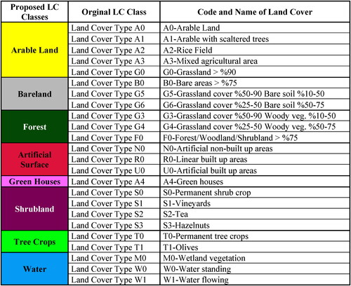
Figure 10. Reference map for a small part of the AOI before (left) and after (right) the application of the negative buffer on the map.

Vector data belonging to the created classes were converted to raster data format. −10 m negative buffering process (erosion) was applied to each class in the raster data, and noise and border pixels caused by the borders between classes were eliminated with this process (Figure10).

3.3. Machine learning and classification

Light GBM machine learning algorithm in the Eo-Learn library was used in the classification process. The Light GBM machine learning algorithm is available by default in this version of the Eo-Learn library, where the classification process is performed. LightGBM is a boosting algorithm based on decision tree algorithms developed in 2017 as part of the Microsoft DMTK (Distributed Machine Learning Toolkit) project. The method was given the prefix ‘Light’ because it is a high processing speed algorithm, as the name implies (Üstüner et al. 2020). Compared to other boosting algorithms, it has advantages such as high processing speed, large data processing, less resource (ram) usage, high prediction rate, parallel learning and GPU learning support (Guolin et al. 2017). The leaf-oriented expansion of the data during the training phase distinguishes the Light GBM algorithm from other algorithms. The leaf-oriented strategy has a lower error rate and allows for faster learning (Li et al. 2019). Hyperparameter optimization is the process of finding the most suitable parameter combination according to the success criteria determined for a machine learning algorithm. With hyperparameter optimization, it is aimed to achieve high success of the model and to balance the complexity of the model and to provide the balance of over and under-learning. LightGBM has many model parameters that need to be tuned, such as boosting type, min child sample, max bin, and seed. As a boostingtype, we chose GOSS (Bentéjac et al. 2021). The parameters were tuned by the trial and error method, and they are listed Table 2.

Table 2. Light Gradient Boosting Machine (LightGBM) parametres.

Parametre	Value
Boosting type	GOSS
Minimum child sample	377
Number of boosted trees to fit	263
Max depth	7
Maximum tree leaves	81
Max bin	255
Seed	42

4. Experimental results and discussion

After determining the optimum parameter of the algorithm to be used in the classification process, the k-fold cross validation method was used. The k-layer verification method allows to see whether the high performance of the model is random or not (Ron 1995). In this method, the data set is divided into k parts and k-1 subsets are used to train the model, and the remaining subset is used to calculate the accuracy of the model. The process is repeated k times, each time using a different piece of training and test data. (Kohavi 1995). In this study, the K value was taken as 5 and 80% of the reference data was used as training data and 20% as test data in the classification. For each k (k1, …, k5) value, the training and test data were automatically selected at the determined percentages by the cross validaiton method. By using Recall and Precision of each class, and the F1 score values, which are the harmonic average of these two values, the overall accuracy was calculated (Table 3).

Table 3. F1 score, recall and precision of classification results.

Class Name	Recall	Precison	F1
Arable land	0.95	0.96	0.95
Water	0.97	0.96	0.96
Artificial surface	0.95	0.95	0.93
Bare land	0.95	0.93	0.94
Shrub land	0.88	0.90	0.88
Forest	0.90	0.87	0.88
Tree crops	0.78	0.73	0.75
		Overall Accuracy %92.2

When the results of the accuracy analysis are examined, it is seen that the arable land, water, artificial surface and bare land classes are above the 90% accuracy value. By examining the Tree crops class, it was discovered that nearly 20% of the class was mixed with the Forest class. When the aforementioned situation is examined, it has been concluded that the evergreen olive trees in the tree crops class and the forest areas are mixed. The overall accuracy in the study is 92.2%. Of the approximately 2230 km² working area, 44.97% is arable land 1002,67 km², %31.84 is forest 709,7 km², %12.83 is bare land 286,11 km², % 1.96 is shrubland 44,03 km², %3.02 is water 67,67 km², %2.75 is artificial surface 61,75 km² and %2.55 is tree crop areas 57,28 km² (Figure 11).

Figure 11. Confusion matrix for classification.

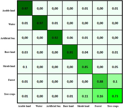
When each class is examined individually, arable land, water, artificial surface, and bareland have an accuracy of 95%, followed by the Forest class with 90%. As can be seen in the error matrix (Figure 11) the shrubland class is mixed with the arable land class to some extent, and the forest class is mixed with the tree crops class at a low rate. On the other hand, fruit trees mixed with forest and shrub land areas give the lowest score and it will be analyzed why the accuracy is low in these classes.

A new study will be conducted both in this study area and in a different area, using different indices and additional bands to improve the mixing classes and increase their accuracy. Since 17 different images are taken throughout the year and the land cover classification cannot change rapidly depending on time like the crop pattern classification, it is unlikely that the classification result will increase in increasing the temporal resolution (5-day). Using the same data set, classification will be performed using the deep learning method, and a comparison with the LightGBM algorithm from the library will be performed.

The classification result also demonstrates that the method is applicable in a variety of fields, as it has a high level of accuracy both in general and on a class basis. The Land Use Land Cover classes that emerged from classification and the LPIS physical blocks were compared and evaluated (Table 4).

Table 4. Comparison of LPIS physical blok and classification results.

Class Name	LPIS-2015 (hectare)	LU/LC Classification-2020 (hectare)
Arable land	100267	105185
Water	6767	5749
Artificial surface	6175	6197
Bare land	28611	29616
Shrub land	4403	3219
Forest	70970	68701
Tree crops	5728	4254
	222921	222921

When the LPIS classes drawn in 2015 are compared with the classification results of 2020; it was determined that the arable land class increased by 4918 hectares (4.9%), the water class decreased by 1018 hectares (15%), the artificial surface area increased by 22 hectares, the bareland area increased by 1005 hectares (3.5%), the shrubland area decreased by 1184 hectares (27%), the forest area increased by 2269 hectares decreased (3.2%), and tree crops area decreased by 1474 hectares (25%).

When the results are examined with physical blocks, classification result and satellite image, it is clear that there is a transition from shrubland, tree crops to arable land class, and some of the forest areas are converted to agricultural lands. It has been determined that approximately 1000 hectares of land in the Water class have been transferred to the bareland class. The reason for this situation was investigated, it was discovered that both the effect of global warming and the unconscious irrigation in the region negatively affected the wetland in the last 5 years.

The open source Eo-Learn library has been shown to provide users with great convenience and time in remote sensing studies with artificial intelligence, in land cover classification, and crop classification, with a ready-made workflow, and it also provides success in the classification study. This library is run with jupyter notebook and is a bit complicated for users, the interface could be simplified even further for end users. This appears to be the only disadvantage of the Eo-Learn library (Figure 12).

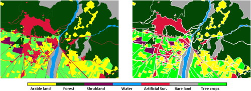
Figure 12. Classification results for the Denizli-Çivril region 2020, based on Eo-Learn library.

5. Conclusion

The use of machine learning algorithms in remote sensing studies has become widespread over time, and time-consuming processing steps and classification processes are made semi-automatic or automated by supporting various ready-made pipeline models, libraries and platforms developed for users. Especially having such libraries or ready-made workflows provides convenience in large areas or regional studies. In this study, the land cover classification of an area of approximately 2230 km² covering Çivril-Baklan Plain within the boundaries of Deniz Province, Çivril, Baklan and Çal districts for 2020 bas made using the python-based open source Eo-Learn library.

Before the classification process, the images had to go through a number of pre-processing processes. Sentinel-2 images with 15-day intervals were used in the study, these images were obtained by dividing into segments (EO-Patch) as a time series integrated with Eo-Learn, instead of being provided individually. This has provided great convenience when both image selection and lead time are taken into account. With the help of the Eo-Learn library, procurement the images to be used in the classification process, identifying and masking the cloudy areas, index-feature extraction using the bands in the images, and image stack operations consisting of the combination of the bands in the images and the extracted indexes are easily performed with the interconnected pipeline models in the open source library.

In the classification process, physical blocks produced from 30 cm orthophoto images in 2015 within the scope of the Land Parcel Identification System were used as reference data, and classes close to each other were grouped as the training data set.

The most significant advantage of physical blocks is that they are drawn precisely on orthophoto images and are subject to external quality control within the scope of the project. The disadvantage is that over the years, some classes may lose their own characteristics and switch to another class qualification. However, it still represents a reliable data as place accuracy training data in the classification process.

After the pre-processing of the images and the preparation of the reference parcels, the land cover classification was made using the LightGBM algorithm in the Eo-Learn Library. As a result of the classification process, the accuracy analyzes were examined, and the overall accuracy was 92.2%, indicating that the study provided high accuracy. Only in fruit trees due to mixing with the forest class, the classification result is poor.

The LPIS system, which is one of the basic components of IACS, is used as a reference system in the management and control of support payments. In our country, LPIS data was created in 2015 and needs to be updated. Updating all data at the country scale is a significant workload in terms of time and cost, and it may not be necessary to update every class within the scope of LPIS at the same scale and workload (artificial surface, bareland, water). However, the areas with different land cover classes within the agricultural areas need to be updated (arable land, shrub land, tree crops etc.) With the Eo-Learn library, the steps of image procurement, satellite image pre-processing, selection of training data and classification with machine learning can be done quickly, easily and safely on a regional or country scale, saving time with interconnected and integrated pipeline models. By comparing the classes that emerged as a result of the classification made and the LPIS classes, the workload that will occur in the Ministry for updating the LPIS data will be determined, and the land cover classification will form the basis for which areas to focus on most and where to start due to possible changes.

Author contributions

Fatih Fehmi ŞİMŞEK (Conceptualization, Methodology, Data curation, Writing-Original draft preparation, Validation), Süleyman Savaş DURDURAN (Methodology, Review and Editing).

Acknowledgments

The authors would like to thank the General Directorate of Agricultural Reform for providing the physical blocks used in the study and from Sinergise Company general manager Grega Milcinski and Matic Lubej for their support regarding the Eo-Learn library.

Disclosure statement

No potential conflict of interest was reported by the authors.

Additional information

Funding

The authors would like to thank the General Directorate of Agricultural Reform for providing the physical blocks used in the study and from Sinergise Company general manager Grega Milcinski and Matic Lubej for their support regarding the Eo-Learn library.

References

- Aksever F, Eroğlu A. 2016. Çivril-baklan (Denizli) ovasında yeraltı suyuna iklim değişikliğinin etkisi. Mehmet Akif Ersoy Üniversitesi Fen Bilimleri Enstitüsü Dergisi. 7(1):11–26.
- Aleksandrov M, Visnjic J. 2020. Land cover monitoring system. Medium. [accessed 2021 Apr 13] https://medium.com/sentinel-hub/land-cover-monitoring-system-84406e3019ae.
- Bentéjac C, Csörgő A, Muñoz GM. 2021. A comparative analysis of gradient boosting algorithms. Artif Intell Rev. 54(3):1937–1967. springer netherlands).
- Candido C, Blanco AC, Medina J, Gubatanga E, Santo A, Ana RS, Reyes RB. 2021. Improving the consistency of multi-temporal land cover mapping of Laguna lake watershed using light gradient boosting machine (LightGBM) approach, change detection analysis, and Markov chain. Remote Sens Appl: Soc Environ. 23(5):100565.
- Crist EP, Cicone RC. 1984. A physically-based transformation of Thematic Mapper data the TM Tasseled Cap. IEEE Trans Geosci Remote Sensing. GE-22(3):256–263.
- Efthimiou N, Psomiadis E, Papanikolaou I, Soulis KX, Borrelli P, Panagos P. 2022. Developing a high-resolution land use/land cover map by upgrading CORINE’s agricultural components using detailed national and pan-European datasets. Geocarto Int. 37(4):1–36.
- Eitel JH, Vierling LA, Litvak MA, Long DS, Schulthess U, Ager AA, Krofcheck DJ, Stoscheck L. 2011. Broadband, red-edge information from satellites improves early stress detection in a new mexico conifer woodland. Remote Sens Environ. 115(12):3640–3646.
- Foerster S, Kaden K, Foerster M, Itzerott S. 2012. Crop type mapping using spectral-temporal profiles and phenological information. Comput Electron Agric. 89(4):30–40.
- Gomez C, White JC, Wulder MA. 2011. Characterizing the state and processes of change in a dynamic forest environment using hierarchical spatio-temporal segmentation. Remote Sens Environ. 115(7):1665–1679.
- Guolin K, Men Q, Finley T, Wang T, Chen W, Ma W, Ye Q, Liu TY. 2017. LighGBM: a highly efficient gradient boosting decision tree. 31st Conference on Neural Information Processing Systems (NIPS 2017), California; p. 3147–3155.
- Harvolk S, Kornatz P, Otte A, Simmering D. 2014. Using existing landscape data to assess the ecological potential of miscanthus cultivation in a marginal landscape. GCB Bioenergy. 6(3):227–241.
- Inan HB, Sagris V, Devos W, Milenov P, Oosterom PV, Zevenbergen J. 2010. Data model for the collaboration between land administration systems and agricultural land parcel ıdentification systems. J Environ Manage. 91(12):2440–2454.
- Jarray N, Abbes A, Rhif M, Chouikhi F, Farah IR. 2021. An open source platform to estimate soil moisture using machine learning methods based on eo-learn library. In: International Congress of Advanced Technology and Engineering, ICOTEN; p. 21–25.
- Kalkan K, Maktav D. 2016. Landsat-8 görüntülerinden gölge ve bulut belirleme. In: VI. Uzaktan Algılama ve Coğrafi Bilgi Sistemleri Sempozyumu, Adana; p. 5–7.
- Karlsen SR, Stendardi L, Tømmervik H, Nilsen L, Arntzen I, Cooper EJ. 2021. Time-series of cloud-free sentinel-2 ndvi data used in mapping the onset of growth of central spitsbergen, svalbard. Remote Sensing. 13(15):3031–3014.
- Kauth RJ, Thomas GS. 1976. The tasselled cap a graphic description of the spectral–temporal development of agricultural crops as seen by Landsat. In: Symposiumon Machine Processing of Remotely Sensed Data. Vol. 76; p. 41–51.
- Kohavi R. 1995. A study of cross-validation and bootstrap for accuracy estimation and model selection. In: International Joint Conference of Artificial Intelligence.
- Kriegler FJ, Malila WA, Nalepka RF, Richardson W. 1969. Preprocessing transformations and their effect on multispectral recognition. Remote Sens Environ. 6:97–132.
- Li W, Ding S, Chen Y, Wang H, Yang S. 2019. Transfer learning-based default prediction model for consumer credit in China. J Supercomput. 75(2):862–884.
- Li W, Du Z, Ling F, Zhou D, Wang H, Gui Y, Sun B, Zhang X. 2013. A comparison of land surface water mapping using the normalized difference water index from TM, ETM + and ALI. Remote Sens. 5(11):5530–5549.
- Lu D, Weng Q. 2007. A survey of ımage classification methods and techniques for ımproving classification performance. Int J Remote Sens. 28(5):823–870.
- Lubej M, Aleksandrov M, Batic M, Kadunc M, Milcinski G, Peressutti D, Zupanc A. 2019. Spatio-temporal deep learning: an application to land cover classification. In: Living Planet Symposium. Milano; p. 2–5.
- Lubej M. 2018. Land cover classification with eo-learn: part-1. Medium. [accessed 2021 May 20] https://medium.com/sentinel-hub/land-cover-classification-with-eo-learn-part-1-2471e8098195.
- Lüker-Jans N, Simmering D, Otte A. 2016. Analysing data of the ıntegrated administration and control system (ıacs) to detect patterns of agricultural land-use change at municipality level. Landscape Online. 48(1):1–24.
- Luketic N, Milenov P, Devos P. 2015. Management of layers in LPIS- JRC validated methods, reference, methods and measurements report, Joint Research Centre, DS-CDP-2015-10.
- Mcfeeters SK. 1996. The use of the normalized difference water ındex (ndwı) in the delineation of open water features. Int J Remote Sens. 17(7):1425–1432.
- Papadakis I, Papetheodorou I, Faria Viegas H, Milionis N, Szymura M, Huth J, Sniter K, Bortnowschi R, Resegotti R. 2016. The Land Parcel Identification System: a useful tool to determine the eligibility of agricultural land – but its management could be further improved. Eur Court Audıtors-Spec Rep. 25(59):35–38.
- Peressutti D. 2018. Introduction eo-learn. Medium [accessed 2021 Feb 15] https://medium.com/sentinel-hub/introducing-eo-learn-ab37f2869f5c.
- Račič M, Oštir K, Peressutti D, Zupanc A, Zajc LC. 2020. Application of temporal convolutional neural network for the classifıcation of crops on Sentınel-2 time series. Int Arch Photogramm Remote Sens Spatial Inf Sci- ISPRS Arch. 43(B2):1337–1342.
- Ron K. 1995. A study of cross-validation and bootstrap for accuracy estimation and model selection. In: International Joint Conference of Artificial Intelligence, Stanford, CA.
- Schowengerdt RA. 2007. Remote sensing: models and methods for image processing. 3rd ed., Elsevier; p. 250–254.
- Tomlinson SJ, Dragosits U, Levy PE, Thomson AM, Moxley J. 2018. Quantifying gross vs. net agricultural land use change in great britain using the ıntegrated administration and control system. Sci Total Environ. 628–629:1234–1248.
- Üstüner M, Abdikan S, Bilgin G, Şanlı FB. 2020. Hafif gradyan artırma makineleri ile tarımsal ürünlerin sınıflandırılması. Türk Uzaktan Algılama ve CBS Dergisi. 1(2):97–105.
- Üstüner M, Şanlı FB, Abdikan S. 2015. Spektral band ve bitki indeksi seçiminin ürün deseni sınıflandırma doğruluğuna etkisi: karşılaştırmalı analiz. In: TUFUAB VIII. Teknik Sempozyumu, Konya; p. 16–20.
- Viana CM, Girão I, Rocha J. 2019. Long-term satellite ımage time-series for land use/land cover change detection using refined open source data in a rural region. Remote Sens. 11(9):1104.
- Zha Y, Gao J, Ni S. 2003. Use of normalized difference built-up ındex in automatically mapping urban areas from tm ımagery. Int J Remote Sens. 24(3):583–594.
- Zheng H, Du P, Chen J, Xia J, Li E, Xu Z, Li X, Yokoya N. 2017. Performance evaluation of downscaling sentinel-2 imagery for land use and land cover classification by spectral-spatial features. Remote Sens. 9(12):1274–1142.
- Zhu Z, Woodcock CE. 2012. Object-based cloud and cloud shadow detection in Landsat imagery. Remote Sens Environ. 118:83–94.
- Zupanc A. 2017. Improving cloud detection with machine learning. Medium [accessed 2021 Sep 5]. https://medium.com/sentinel-hub/improving-cloud-detection-with-machine-learning-c09dc5d7cf13.