DSMFFNet: Depthwise separable multiscale feature fusion network for bridge detection in very high resolution satellite images

Abstract

Bridge detection methods based on deep learning have many parameters, complex calculations, and serious errors and missed detections for multiscale bridges. To solve the above problems, a depth-wise separable multiscale feature fusion network (DSMFFNet) is proposed for efficient and accurate bridge detection in very high resolution satellite images (VHR). First, depth-wise separable convolution was used to build a backbone feature extraction network to extract the bridge features. Second, to better match bridges of different scales, multiscale receptive fields were obtained by multibranch parallel dilated convolution at the last layer of the feature map. Then, to make full use of the details and semantic information of the bridges at different depths, the three effective feature layers of the bridges at different levels are fused by a multiscale feature pyramid. The experimental results showed that the mean average precision (mAP) and frame per second (FPS) of the proposed method reach 94.26% and 60.04%, which can lead most of the mainstream object detection networks in accuracy and speed and can be integrated into the mobile end to complete the task of high-precision and fast bridge detection.

Keywords:

• Depthwise separable convolution
• object detection
• bridge
• multiscale object
• feature fusion

SUBJECT CLASSIFICATION CODES:

• O18
• Urban
• Rural
• Regional
• Transportation Analysis
• Housing
• Infrastructure
• R42
• Government and Private Investment Analysis
• Road Maintenance
• Transportation Planning
• R58
• Regional Development Planning and Policy

1. Introduction

As an important transportation facility, bridge is the key transportation hub between land and water. During the war, many important military forces are often deployed around the bridge, so the bridge and its surrounding facilities are key military objects, which has important strategic and tactical significance. Second, with the gradual acceleration of urbanization, bridges play an increasingly important role in urban planning and construction. They are the most needed and indispensable part in urban planning and construction. As a large man-made feature, the bridge is also the most easily changed object in the geographic database. Its updating and maintenance play a guiding role in urban planning and construction. Using image processing technology to automatically detect bridges can not only speed up the detection speed, but also improve the detection accuracy. It has broad development prospects and important research significance in both military and civil affairs. VHR plays an important role in industry, agriculture, military, economy and other fields, and have also become an important data source for object detection (Cao et al. 2020; Yao et al. 2021). However, due to environmental factors and imaging conditions, there are great differences in bridge object background and bridge shape in VHR, so it is difficult to distinguish bridges in different VHR by using unified features. At the same time, the sizes of the different bridges in an image vary greatly, and an imbalance of positive and negative samples easily appears, which increases the difficulty of bridge detection. Therefore, it is of great significance to research the high precision and fast detection of bridges.

Currently, bridge detection can be divided into two main categories: (1) Bridge detection methods based on traditional methods. These methods mainly combine human-designed feature operators (i.e. templates) to detect objects using sliding windows, such as edge extraction operators Sobel, prewitt, robert, etc. However, in practical scenarios, feature extraction is often difficult due to the reliance on certain specific features (e.g. water bodies, coastlines, etc.), or due to imaging conditions and human subjective factors that lead to bridge misdetection and omission. For example, Fan et al. (2006) proposed a cross-entropy-based feature extraction and object detection method for river areas, which can be used for bridge detection in river areas. However, the feature parameters proposed by this method depend too much on the water characteristics under specific conditions, and the detection robustness of bridges in VHR with different backgrounds is poor. Jiang et al. (2006) proposed a multisource remote sensing image fusion method for automatic detection of bridge objects that can effectively detect bridges in complex and large scenes. However, near infrared, panchromatic and SAR images need to be fused. Additionally, different data in the same area are difficult to obtain, and the work is tedious, making it difficult to achieve efficient and automatic detection of bridges. Sithole and Vosselman (2006) proposed a method to detect bridges in laser scanning data. Topological information was used to identify the seed points of bridges, and then a threshold value was set to detect a single bridge using seed points. Bridges with different shapes can be effectively detected, but poor threshold setting will misclassify riverbanks into bridges, which will affect the accuracy of bridge positioning. D. Chaudhuri and Samal (2008) proposed a method to detect water bridges using multispectral images, classifying the images as water, concrete and background, but it cannot address the problem of imbalance between positive and negative samples. When the bridge object is very small or the image contains noise, classification errors will occur. Huang et al. (2018) proposed the scene semantic SAR image bridge detection algorithm, which can effectively suppress coherent spots. Noise reduces the missed and false detections of bridges, but it is effective only for bridges on water. (2) Bridge detection methods based on deep learning. For example, a bridge detection network based on a multiresolution balance and attention mechanism was proposed by Chen et al. (2020), which can effectively address the problem of bridge detection in SAR images, but its model is complex and low in accuracy. Zhou (2020) proposed an optical remote sensing image bridge detection method with a dual attention mechanism to effectively solve the problem of low target detection accuracy in complex backgrounds, but the detection speed must be improved. Sun (2022) proposed a high spatial resolution automatic detection of bridges with high spatial resolution remote sensing images based on random erasure and YOLOv4, which effectively enhances the accuracy of bridge detection as well as the robustness of the network. However, the method still suffers from the problem of slow detection speed. However, the above methods often cannot balance speed and accuracy at the same time.

In response to the above problems, DSMFFNet is proposed for bridge detection in this paper. The main contributions of DSMFFNet can be summarized as follows:

1. Depthwise separable convolution is used to build a backbone network; it can greatly reduce the network parameters, reduce the computing costs, and increase the operating speed of the network at the same time, providing the possibility of obtaining real-time and efficient bridge detection;

2. Multibranch parallel dilated convolution is used to obtain different sizes of receptive fields, retain the detailed information of small objects, and improve the detection ability of multiscale bridges;

3. To make full use of the bridge feature information in different level feature maps, a multiscale feature pyramid is used to achieve cross-level network feature fusion.

The remaining sections are organized as follows: The proposed method is introduced in Section 2, including depthwise separable convolution to build the backbone network, multibranch parallel dilated convolution to expand the field of perception, and a multiscale cross-layer feature pyramid for feature fusion. In Section 3, bridge detection experiments are conducted with different networks, and the experimental results are analyzed. Conclusions and prospects are summarized in Section 4.

2. Related works

As an important part of remote sensing image interpretation, object detection methods have been receiving more and more attention. This section reviews the object detection related work done by previous authors and focuses on two stages of object detection framework development: traditional object detection stage and deep learning object detection stage.

2.1. Traditional object detection

The traditional object detection algorithm focuses on the selection of object features, and the reliability of the object detection results depends entirely on the quality of the feature representation effect. The process can be summarized in three steps: first, selecting the region of interest and extracting the candidate regions using the sliding window method, then extracting the specific features within these candidate regions, and finally classifying and recognizing them using the corresponding classifier.

Papageorgiou et al. (1998) used wavelet transform to extract image features to achieve object detection in static images. However, the wavelet transform faded out of the object detection field because it is not rotationally invariant. Viola and Jones (2004) proposed the VJ detector, which combines three key techniques: ‘integral image’, ‘feature selection’ and ‘cascade detection’ that lay the foundation for subsequent research on various types of detectors. Subsequently, Lowe (2004) proposed the Scale-Invariant Feature Transform (SIFT), which can effectively cope with image rotation, translation and scaling, thus achieving effective matching of objects or scenes from different viewpoints. The following year, Dalal and Triggs (2005) improved SIFT and shape context and proposed the Histogram of Oriented Gradient (HOG). This method has the advantages of fast feature extraction and strong generalization ability, and is a pre-processing process for many single-category detection and multi-category detection.

2.2. Deep learning methods

Traditional object detection methods rely on manually designed features or a priori knowledge for object detection, and therefore have low robustness and cannot be generalized to multi-category objects, which basically reached saturation around 2010. Hinton’s team (2012) proposed the AlexNet deep learning model, which gained unprecedented success and marked the advent of the era of deep learning. In the field of deep learning, object detection methods mainly include ‘two-stage object detection’ and ‘single-stage object detection’.

(1) Two-stage object detection methods

Girshick et al. (2014) proposed R-CNN to improve the detection accuracy significantly, but the detection speed was greatly slowed down by generating thousands of proposal on the image for each detection. The following year, to improve the complex training process of R-CNN and increase the detection speed, He et al. (2015) proposed a Spatial Pyramid Pooling Networks (SPPNet). In the same year, Girshick (2015) proposed the Fast R-CNN detector, which successfully combined the advantages of R-CNN and SPPNet to significantly speed up the training process and testing process, and also further improve the detection accuracy. Shortly afterwards, Ren et al. (2017) proposed the Faster R-CNN, which overcame the speed bottleneck of Fast R-CNN computing, improved the computing efficiency and realized end-to-end object detection. Subsequently, excellent two-stage object detection networks such as R-FCN (Dai et al. 2016), FPN (Lin et al. 2017), etc. were born, but they always failed to meet the needs of real-time object detection.

(2) One-stage object detection methods

These methods reduce the object detection problem to a regression problem, and compared to two-stage methods, regression-based methods omit the region proposal generation process, making the object detection method faster and more effective. OverFeat proposed by Pierre (2013) integrates the recognition localization and detection tasks, and is considered a pioneer of one-stage object detection, laying the foundation for subsequent research on one-stage detection. Redmon J et al. (2015) proposed YOLO, which used a single neural network to process the whole image and was the first formal one-stage detector in the deep learning era. In the same year, Liu et al. (2016) proposed SSD, which introduces a priori frames to balance detection speed and accuracy, and Lin et al. (2017) proposed RetinaNet, which introduces a focal loss function and enables the detector to focus on samples that are difficult to classify. Later, YOLOv2 (Redmon et al. 2017), YOLOv3 (Redmon J et al. 2018) and YOLOv4 (Bochkovskiy et al. 2020) were proposed one after another to improve the low recall rate of YOLO, which continuously improved the backbone network and feature fusion module to achieve faster and more accurate object detection.

3. Methodology

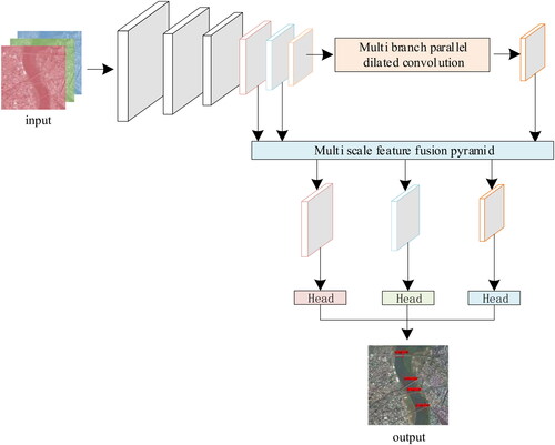
A bridge detection method is proposed based on DSMFFNet. First, a depth-wise separable convolution (Howard et al. 2017) is used to construct the bridge feature extraction network to reduce the network parameters and compress the network model in DSMFFNet. Second, multibranch parallel dilated convolution is applied to enlarge the receptive field on the last layer of the bridge feature map to further extract the features of bridges at different scales. Then, multiscale features are combined with pyramids to achieve cross-level bridge feature map fusion, making full use of the details and semantic information of different bridge feature maps. Finally, the results of bridge detection are output through the detection head. The flow chart of DSMFFNet is shown in Figure 1.

Figure 1. The flow chart of DSMFFNet.

3.1. Bridge feature extraction backbone network

The most direct way to improve the performance of bridge detection networks is to increase the depth and width of the network. However, with the increasing depth of the network, the gradient explosion problem in the backpropagation process also follows (Yu et al. 2021). The parameters that the network needs to learn become increasingly massive, and the large number of parameters is prone to overfitting (He et al. 2016; Zheng et al. 2020), which will affect the performance of the bridge detection. Second, the complex network structure and many parameters have high requirements for the computer hardware, and the data in the same batch of incoming networks are severely limited (Ioffe and Szegedy 2015).

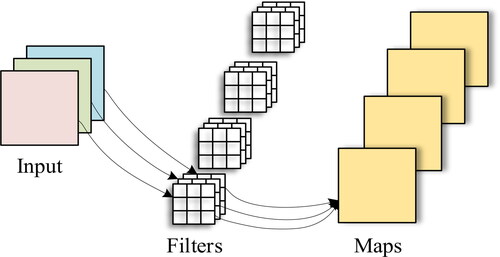
As the best choice for extracting target features, convolutional neural networks (CNNs) have been widely used in various object detection methods (Tarhan and Akar 2018). Bridge detection is conducted by using the conventional convolution that constitutes the CNN. First, the input feature maps of each channel are convoluted with the corresponding convolution kernel, and then, the results are added and output. The process is shown in Figure 2. For the $D_F\times D_F\times M$ bridge input image, using N dimensions of a $D_K\times D_K\times M$ standard convolution kernel is used for convolution operations. M is the number of input channels, and N is the number of convolution kernels, in other words, the number of output channels. When convoluting with standard convolution kernels, the step size is 1, padding is used, and the size of the output feature maps is $D_F\times D_F\times N.$ The amount of calculation is (1) $$P_1=D_F\times D_F\times D_K\times D_K\times M\times N$$(1) where D_F is the width of the input image, D_K is the width of the output image, M is the input feature map dimension and N is the output feature map dimension.

Figure 2. Schematic diagram of conventional convolution.

Depth-wise convolution and pointwise convolution, as shown in Figure 3. Depthwise convolution is a noncross-channel convolution in which each channel of the feature map corresponds to an independent convolution kernel, each convolution kernel acts only on a specific channel, and the number of channels of the output feature map is equal to the number of channels of the input feature map. For the bridge input image of $D_F\times D_F\times M,$ the convolution is performed using M convolution kernels, and the convolution calculation is performed only within each channel. The information between the channels is not additive. Finally, M feature maps are output. Thus, the amount of calculation for the depthwise convolution is (2) $$P_2=D_F\times D_F\times M\times D_K\times D_K$$(2)

Figure 3. Depthwise separable convolution.

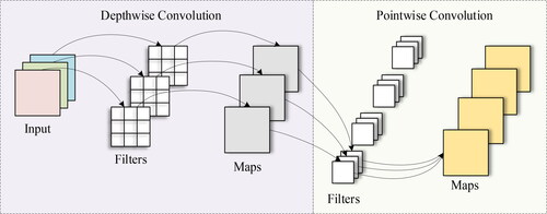
Pointwise convolution is used for feature merging, and dimension change through 1 × 1 convolution traverses the characteristics of each point, while collecting spatial information of multiple channels and realizing cross-channel information fusion. This approach makes up for the problem that each channel feature is separated from every other channel feature in the process of depthwise convolution. Second, each pointwise convolution layer follows the batch normalization (BN) and ReLU layers, effectively increasing the nonlinear variation of the model, thereby enhancing the generalization ability of the model. For the output feature map from depthwise convolution, pointwise convolution uses N convolution kernels of size 1 × 1×M to conduct the convolution operation, and the final output feature map size is $D_K\times D_K\times N.$ The amount of calculation is (3) $$P_3=D_F\times D_F\times M\times N$$(3)

Then, the ratio of the depthwise separable convolution to the conventional computational effort is (4) $$\frac{P_2+P_3}{P_1}=\frac{D_F\times D_F\times M\times D_K\times D_K+D_F\times D_F\times M\times N}{D_F\times D_F\times D_K\times D_K\times M\times N}=\frac{1}{N}+\frac{1}{D_K^2}$$(4)

N is the number of output channels. Normally, when N is large, $\frac{1}{N}$ is negligible. Taking D_k=3 as an example, $\frac{1}{D_K^2}=\frac{1}{9},$ in other words, the calculation of the depthwise separable convolution is only $\frac{1}{9}$ of that of the conventional convolution, which greatly improves the computational efficiency of the model.

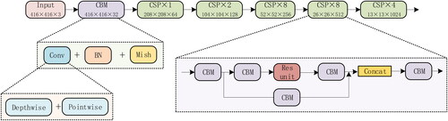
To reduce the number of parameters and the computation, a bridge feature extraction network that combines depthwise separable convolution and CSPDarknet53 (Wang et al. 2020; DSC-CSPDarknet53) is proposed. DSC-CSPDarknet53 consists mainly of Convolution + Banch Normalization + Mish (CBM) (Ioffe and Szegedy 2015; Misra 2019) and Cross Stage PartialX (CSPX) modules. As shown in Figure 4, the CBM module consists of a convolution layer, a batch standardized convolution, and a Mish excitation function. The convolution layer consists of a depthwise convolution and a pointwise convolution, in other words, a depthwise separable convolution layer. The CSPX module divides the bridge feature map into two parts: the first part passes through the CBM module and X residual components (Res units) (He et al. 2016); the second part combines Concat directly with the first part. DSC-CSPDarknet integrates gradient changes in the bridge feature map, effectively enhances the learning ability of the network, and uses depthwise separable convolution for all convolution layers, which reduces the computational effort while guaranteeing high accuracy.

Figure 4. The network structure of DSC-CSPDarknet53.

3.2. Multibranch parallel dilated convolution

Receptive fields (Takahashi and Mitsufuji 2020) represent the spatial extent of the input image that corresponds to the unit pixel on the output feature map. In CNNs, the size of the receptive field is directly affected by the size of the convolution kernel, and the size of the receptive field directly affects the detection of objects at different scales (Luo et al. 2017). Therefore, the single-scale receptive field generated by a single-size convolution kernel cannot be used to detect multiscale bridges in the same image. Although operations such as downsampling and pooling can effectively expand the receptive field, they can reduce the spatial resolution and prevent small-scale bridge information from being reconstructed (Zhang et al. 2020). Using the dilated convolution method, different scale receptive fields can be obtained, which can solve the problem of low detection accuracy of multiscale bridges.

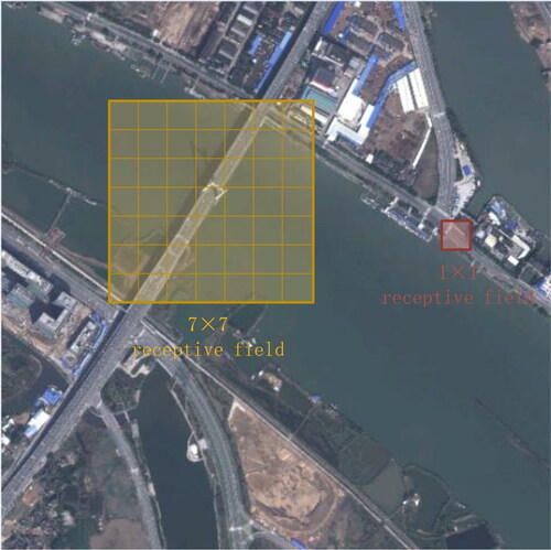
The 1 × 1 convolution kernel can produce a 1 × 1 receptive field, which is suitable for detecting small bridges, as shown in the red box on the right side of Figure 5, while the 1 × 1 receptive field cannot cover large bridges. As shown in the yellow box on the left side of Figure 5, only 7 × 7 receptive fields can be used for detection. If the whole image uses a 7 × 7 receptive field, it will contain a large amount of irrelevant background when detecting small bridges, which will lose the detailed information of small bridges and will not be conducive to the acquisition of object features.

Figure 5. The receptive fields corresponding to objects of different scales.

Dilated convolution (Chen et al. 2018) refers to the introduction of a dilated rate into a conventional convolution, which is the distance between each pixel in the convolution kernel. The dilated rate of the conventional convolution is 1. Figure 6(a) is a conventional convolution diagram, and Figure 6(b) is a dilated convolution diagram. The convolution kernel size after adding a dilated kernel is (5) $$k\prime =n\times (k-1)+1$$(5)

Figure 6. Diagram of dilated convolution.

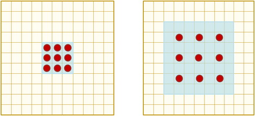
The receptive field size after the dilated convolution is (6) $$r=\left[\left(n-1\right)\times \left(k+1\right)+k\right]\times \left[\left(n-1\right)\times \left(k+1\right)+k\right]$$(6) where k‘ is the size of the convolution kernel after adding dilates, n is the dilated rate, and k is the size of the conventional convolution kernel. Then, for the conventional convolution in Figure 6(a), with a convolution kernel size of 3 × 3 and a dilated rate of 1, the obtained receptive field is shown in the blue part of the figure with a size of 3 × 3. The pixels involved in the calculation, i.e. containing the weights, are the nine red dots in the figure. For the dilated convolution in Figure 6(b), the convolution kernel size is 5 × 5, the dilated rate is 2, and the receptive field size is 7 × 7. The pixels involved in the calculation, i.e. containing the weights, are also only the 9 red points in the figure, and the weights of the other points are 0. Therefore, dilated convolution can solve the problem of spatial information loss of feature maps caused by pooling operations and expand the receptive field without adding additional parameters and computations (Zhu et al. 2018).

Because the dilated part of the dilated convolution does not participate in the sampling operation, the extracted bridge information is discontinuous (Liu S et al. 2017). To extract the features of the dilated part, more accurately locate the position information of bridges with different scales, and further save computing resources, combined with the idea of the inception structure (Szegedy et al. 2015, 2016), the conventional convolution and dilated convolution operations of different sizes are connected in series and then connected in parallel to form a group of convolution modules with asymmetric structures, which can ensure the consistent size of the feature map output by each parallel branch. Figure 7 shows a schematic diagram of multiscale parallel dilated convolution.

Figure 7. Multi branch parallel dilated convolution.

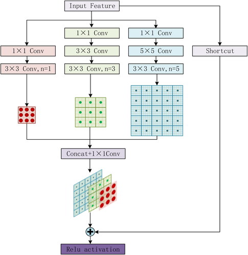
To reduce the amount of calculation, the three parallel branches first use a 1 × 1 convolution to reduce the number of channels; second, to meet the requirements of object detection of different sizes, the two parallel branches use 3 × 3, 3 × 3, and 5 × 5. For the size of the convolution kernel, the corresponding dilated ratios are 1, 3, and 5, respectively. Conventional convolution can extract the features of the dilated part, which can not only obtain continuous information but also obtain receptive fields of different sizes; finally, the feature maps of different scales are concatenated and added with the short edge of the input feature map to output the feature map.

3.3. Multiscale feature pyramid

A network with good performance usually has a deeper network layer, and the feature maps of different depths in the network can express multiscale features (Yu et al. 2021). However, because of the depth differences of the feature maps, the feature expression ability is also different (Liu Y 2020). For the bridge detection network, a low-level feature has higher resolution and contains more bridge location and detailed information. However, due to less convolution, it has lower semantics and more noise. High-level features have stronger bridge semantic information, but the resolution is very low and the perception of details is poor. In other words, with the deepening of the level of the convolutional neural network, the abstract features become increasingly obvious, but the shallow spatial information is gradually lost (Tong et al. 2020; Xu and Wu 2021). Therefore, directly predicting bridge objects of different scales by feature maps of different depths within the network does not yield good detection results, and it is necessary to construct cross-level feature pyramids using feature maps of different depths to realize multiscale feature fusion (Shi et al. 2021).

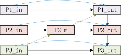
Figure 8 is a multiscale cross-layer feature pyramid structure diagram. The backbone feature extraction network includes six main convolution modules to obtain six convolution maps of different sizes. The last three-layer feature maps P1, P2 and P3 are used 1 respectively × 1. Adjust the number of channels, to obtain feature layers P1_in, P2_in, and P3_in. P3_in is upsampled and stacked with P2_in to obtain P2_m, and P2_m is upsampled and stacked with P1_in to obtain P1_out. P1_out is downsampled and stacked with P2_in and P2_m to obtain P2_out, and P2_out is downsampled and stacked with P3_in to obtain P3_out. All of the above operations have conducted feature fusion, and all of them contribute to multiscale feature fusion. Second, a connection is directly constructed between the input feature map and the output feature map of the same scale, which can fuse more abundant features. Finally, the feature map is stacked many times, which makes the pyramid have a more powerful feature representation ability.

Figure 8. Feature pyramid of multiscale cross layer.

The 416 pixels × 416 pixels bridge image shown in Figure 9 contains s × s cells, and the cell where the center position of the object to be measured is located is responsible for detecting that object, using multiple anchor boxes for object bounding box prediction on each cell of the feature map. The anchor boxes are the bounding boxes obtained by clustering the bridge shapes and dimensions in the dataset. (7) $$\{\begin{array}{c}{b}_x=\sigma \left(t_x\right)+c_x\\ b_y=\sigma \left(t_y\right)+c_y\\ b_w=p_w{e}^{t_w}\\ b_h=p_h{e}^{t_h}\\ P_r(\mathit{object})\times \mathit{IOU}(b,\mathit{object})=\sigma \left(t_o\right)\end{array}$$(7)

Figure 9. Anchor Box.

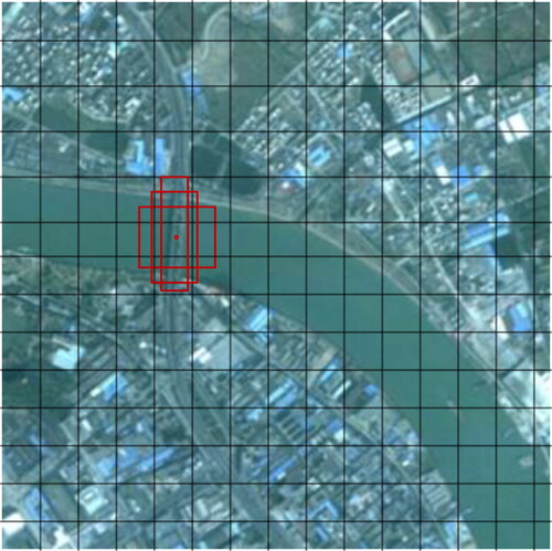
Where, $b_x$′ $b_y$′ $b_w$ and $b_h$ are the center, width, and height of the bounding box, respectively. $c_x$ and $c_y$ are the normalized distance of the current cell from the upper left corner of the image, respectively. $p_w$ and $p_h$ are the width and height of the anchor box, respectively. The relationship between the learning parameters $t_x$′ $t_y$′ $t_w$′ $t_h$ and $t_o$ and the coordinates of the anchor box and the conditional category probability is established using the sigma function $\sigma .$ The bridge feature extraction network performs bridge detection on three scale feature maps, 52 × 52, 26 × 26, and 13 × 13. Finally, the redundant bounding boxes are removed by the Non-Maximum Suppression method to obtain the final bridge object.

4 Experimental results

4.1. Experimental data

The first dataset in this paper adopts the automatic recognition dataset of bridge objects in high-resolution visible light images provided by the 2020 Gaofen Challenge on Automated High-Resolution Earth Observation Image Interpretation (2020). The dataset contains a total of 2,000 VHR ken by Gaofen-2, the resolution of the panchromatic image is 1 m, and the resolution of the multispectral image is 4 m. After the fusion of panchromatic images and multispectral images, the resolution is 1 m. It is including 1,686 images of bridges with an image size of 668 pixels × 668 pixels and 314 images of bridges with 1001 pixels × 1001 pixels, each containing at least one bridge target, mainly bridges over water.

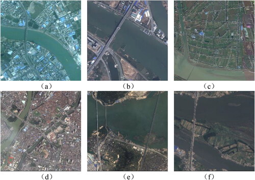
Six bridges under different conditions and scenes are selected for detection in the test set in this paper, as shown in Figure 10. Figure 10(a) shows a conventional bridge with a size of 668 pixels × 668 pixels. The image is clear and the bridge is obvious. Figure 10(b) contains multiple large bridges with relatively different scales, with a size of 668 pixels × 668 pixels. The image background is simple, and the imaging conditions are good. The bridges are obvious but have large differences in size. Figure 10(c) is a large-format remote sensing image with a size of 1001 pixels × 1001 pixels. The background is complex, and the format is large, but the overall image is clear. The pixels of the bridge are relatively small, and the positive and negative samples are extremely uneven. Figure 10(d) is a small bridge detection, and the size is 668 pixels × 668 pixels. The image background is complex, there are a few thin clouds covered, the image color is uneven, the image contains 11 bridge objects, and the largest is only 40 pixels × 40 pixels, compared to an image of 668 pixels × 668 pixels; these can be regarded as small objects. Figure 10(e) is a bridge with a large aspect ratio, with a size of 668 pixels × 668 pixels. The object box will contain considerable background information, which will increase the difficulty of training. Figure 10(f) shows a cross-island bridge with a size of 668 pixels × 668 pixels. This type of bridge crosses the river, and there are land-like areas such as tidal flats or islands in the middle of the river.

Figure 10. Sample dataset1.

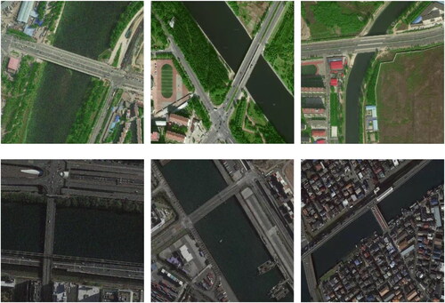
The second dataset in this paper adopt TGRS-HRRSD-Dataset: High Resolution Remote Sensing Detection (Zhang et al. 2019). It contains 3525 bridge object images acquired from Google Earth and Baidu Map with the spatial resolution from 0.15 m to 1.2 m. Each image contains at least one bridge object. The image sizes are not uniform for comparison labs to resize as required by the network. The following figure shows a sample dataset (Figure 11).

Figure 11. Samples of dataset2.

4.2. Experimental design

The experimental environment is based on the Windows 10 operating system, and the computer is configured with an Intel(R) i7–9700k CPU, NVIDIA GeForce GTX1070 Ti graphics card, and 8 GB video memory. A GPU was used for training and testing, and the platform was PyTorch 1.2.0. During the training process, the learning rate gradually decreased. A total of 100 Epochs were trained. The first 50 epochs used an initial learning rate of 1 × 10⁻³, the batch size was set to 16; the next 50 epochs had a learning rate of 1 × 10⁻⁴, and the batch size was set to 8; the IoU threshold was set to 0.5. The dataset was divided into a training set, a validation set and a test set at a ratio of 8:1:1.

When there are fewer training samples in the model, overfitting phenomenon occurs, which reduces the generalization ability of the model. To solve this problem, the Mosaic data augmentation method is used to read 4 images at a time, flip, color gamut change, random scaling, and random cropping of the 4 images. Then a random combination of images and object frames is performed and rescaled to 416 pixels × 416 pixels then, images were transferred to the network. This method can solve the problem of unbalanced proportion of large, medium and small bridges in the dataset, greatly enrich the background of bridge targets, and increase the robustness of the network. In addition, calculating the data of 4 images simultaneously makes the batch-size need not be large, and one GPU can achieve better results (Figure 12).

Figure 12. Mosaic data augmentation.

Network training uses CIOU loss function, which is defined as follows: (8) $$\mathit{LOS}{S}_{\mathit{CIOU}}=1-\mathit{IOU}+\frac{{\rho }^2\mathit{(}\mathit{b},{\mathit{b}}^{gt}\mathit{)}}{c^2}+\alpha \upsilon$$(8) where b represents the prediction box; ${\mathit{b}}^{gt}$ represents the real box; ${\rho }^2\mathit{(}\mathit{b},{\mathit{b}}^{gt}\mathit{)}$ is the Euclidean distance between the prediction frame and the real frame; where c denotes the diagonal distance between the prediction box b and the smallest outer rectangle of the real box ${\mathit{b}}^{gt}.$ (9) $$\mathit{IOU}=\frac{\left|\mathit{b}\cap {\mathit{b}}^{gt}\right|}{\left|\mathit{b}\cup {\mathit{b}}^{gt}\right|}$$(9) where, $\alpha$ is the weight parameter, which is defined as follows (10) $$\alpha =\frac{\upsilon }{1-\mathit{IOU}+\upsilon }$$(10)

Where, $\upsilon$ is used to measure the similarity of aspect ratio, which is defined as follows (11) $$\upsilon =\frac{4}{{\pi }^2}{\mathit{(}\arctan \frac{w^{gt}}{h^{gt}}-\arctan \frac{w}{h}\mathit{)}}^2$$(11) where w, h represents the width and height of the prediction box respectively; $w^{gt},$ $h^{gt}$ represents the width and height of the real box respectively.

The experiment selected mAP, Precision, Recall, F1-score as the objective evaluation index and used the FPS to evaluate the detection speed.mAP is defined as (12) $$\mathit{mAP}=\frac{\sum \mathit{(}\frac{\sum \mathrm{Pr}\mathrm{}\mathit{ecisio}{n}_{\mathrm{c}}}{N_c}\mathit{)}}{N}$$(12) $\mathrm{Pr}\mathrm{}\mathit{ecisio}{n}_{\mathrm{c}}$ is the accuracy of class C objects; The total number of pictures in the object data set is $N_c.$

Precision refers to the proportion of the actual positive sample to the sample predicted to be positive, and is defined as (13) $$\mathit{Pr}\mathrm{}ec\mathrm{}\mathit{ision}=\frac{\mathit{True}P\mathit{ositives}}{\mathit{True}P\mathit{ositives}+F\mathit{alse}\mathit{Positives}}$$(13)

Recall refers to the proportion detected in all positive samples, which is defined as (14) $$\mathit{Re}\mathrm{}\mathit{call}=\frac{\mathit{True}P\mathit{ositives}}{\mathit{True}P\mathit{ositives}+F\mathit{alse}N\mathit{egative}}$$(14)

F1 score is the harmonic average of precision and recall, which is defined as (15) $$F_1=2\frac{\mathit{Pr}\mathrm{}\mathit{ecision}\times \mathit{Re}\mathit{call}}{\mathit{Pr}\mathit{ecision}+\mathit{Re}\mathit{call}}$$(15) where TP represents the positive samples correctly classified, that is, the number of bridges correctly detected; FP represents the negative samples incorrectly classified, that is, the number of non-bridge objects detected as bridges; FN represents the positive samples incorrectly classified, that is, the number of bridges detected as non-bridge objects.

4.3. Experimental results and analysis

To verify the lightweight nature of the proposed method, several object detection methods whose backbone feature extraction networks are Darknet series are compared for model complexity, which are YOLOv3 (Redmon and Farhadi 2018), YOLOv4 (Bochkovskiy et al. 2020), YOLO-tiny, YOLO-Lite (Huang et al. 2018) and the proposed method. The network structures of these methods are similar. YOLO-tiny, YOLO-lite and the proposed method are lightweight networks. Table 1 shows the comparison of the model complexity of the five methods. It can be seen from the table that the parameter quantity and parameter size of the proposed method are greatly reduced compared with the nonlightweight networks YOLOv3 and YOLOv4, and the parameter quantity and parameter size of the proposed method are also suboptimal compared with the lightweight networks YOLO-tiny and YOLO-Lite.

Table 1. Comparison of the model complexity.

Method	Parameter quantity/million	Parameter size/MB
YOLOv3	61.9	236.32
YOLOv4	64	244.29
YOLO-tiny	5.96	22.74
YOLO-lite	12.7	48.42
Proposed	10.8	41.2

Note: the bold numbers in the table are the best results of the method

To compare the accuracy and speed of the proposed method for bridge detection, seven novel methods with excellent performance were selected for comparative experiments, namely, Efficientdet (Tan et al. 2020), Retinanet (Lin et al. 2017), Centernet (Zhou et al. 2019), YOLOv3, YOLOv4, YOLO-tiny and YOLO-lite. And a Multielement Detection Method for Road Traffic in UAV Images Based on Multiscale Feature Fusion: ASFF-YOLOv5 (Qiu et al. 2022). The perspective of the UVA image data it uses is similar to that of satellite imagery. Table 2 shows the results of the training bridge datasets using 8 object detection algorithms and the proposed method. It can be seen from the table that the mAP of the bridge detection ranges from 61.09% to 97.90%, and the FPS ranges from 12.17 to 139.07. The method with the best FPS value is the lightweight network YOLO-tiny, but its mAP is only 81.65%, which makes it difficult to meet the needs of high-precision bridge detection. Although the mAP of the proposed method is only 0.19% higher than that of YOLOv4, the FPS is greatly improved. Precision and Recall are better than the five methods Efficientdet, Retinanet, YOLOv3, YOLO-tiny, and YOLO-lite. F1-score is the second best among the eight compared methods. Therefore, combining the results of Tables 1 and 2, the proposed method not only ensures high-precision detection but also improves the detection speed. Compared with the other fiirst seven mainstream object detection methods, the comprehensive detection ability achieves the best effect. The shortcoming is that compared to ASSF-YOLOv5, a method dedicated to remote sensing images, there is a certain gap in speed and accuracy.

Table 2. Analysis of the main object detection algorithm results in the bridge dataset 1.

Method	mAP/%	Precision/%	Recall/%	F1-score	FPS
Efficientdet	76.67	92.53	75.58	0.83	12.17
Retinanet	78.23	94.08	78.49	0.86	22.98
Centernet	82.07	98.26	82.27	0.90	52.16
YOLOv3	93.82	91.82	92.73	0.92	22.37
YOLOv4	94.07	93.45	95.35	0.94	16.68
YOLO-tiny	81.65	89.44	75.90	0.82	139.07
YOLO-lite	86.57	88.89	88.37	0.89	52.52
ASFF-YOLOv5	97.80	96.20	97.90	0.97	80.00
Proposed	94.26	96.18	94.67	0.95	60.04

Note: the bold numbers in the table are the best results of the method

To verify the ability of the proposed method for bridge detection in different scenarios, six methods are selected for bridge detection. Centernet is the fastest detection method in non-lightweight networks, YOLOv3 and YOLOv4 are high-precision detection methods, and YOLO-tiny and YOLO-lite are lightweight networks. Figures 13–18 show the bridge detection results under different conditions and scenarios. (The values of the test results in the figure are written in Appendix A, see ‘List of test results’ for details.)

Figure 13. Detection results for a conventional bridge.

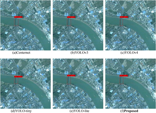
Figure 14. Detection results for multiscale bridges.

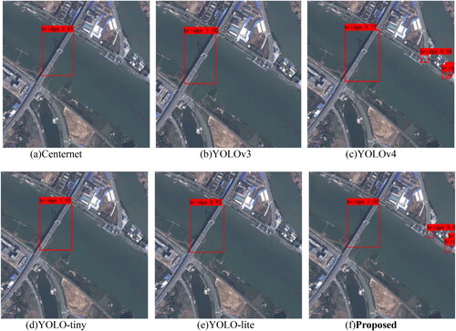
Figure 15. Detection results of multiscale bridges in large-format images.

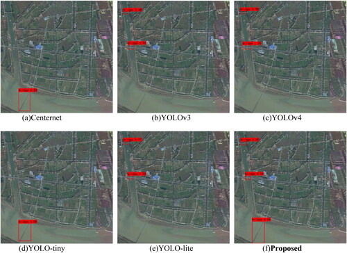
Figure 16. Detection results on small bridges.

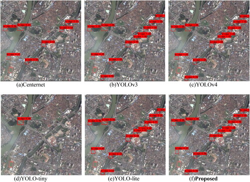
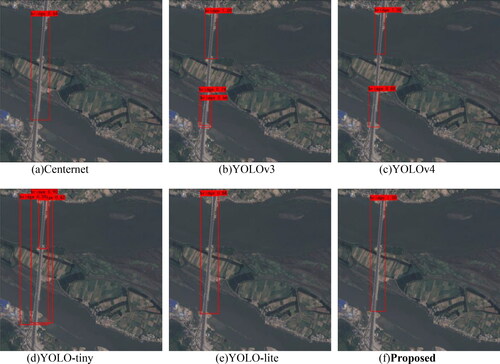
Figure 17. Detection results for bridges with large aspect ratios.

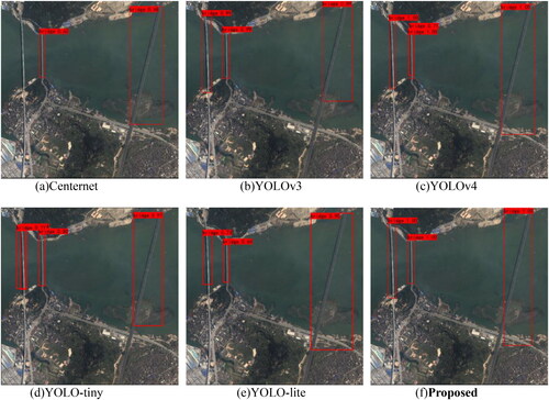
Figure 18. Detection results for cross-island bridge.

(1) Experiment on bridge detection in a simple scenario

The bridge detection results in the simple scenario are shown in Figure 13 Among them, the accuracy of YOLOv3, YOLOv4 and the proposed method can reach 1, and the accuracy of YOLO-tiny and YOLO-Lite can reach 0.94 and 0.81, respectively. Compared with the other five methods, CenterNet has lower accuracy, but it can also successfully detect bridges. The six methods generally have high detection accuracy for conventional bridges, accurate positioning, no false detection and missing detection and have good bridge detection ability.

(2) Experiment on multiscale bridge detection

The detection results of bridges with multiple scale differences in the same image are shown in Figure 14. Among them, Centernet, YOLOv3, YOLO-tiny and YOLO-Lite do not have the ability to perform multiscale bridge detection. For multiscale bridges in the same image, only large and obvious bridges can be detected. YOLOv4 can detect three bridges with different scales, but the overall accuracy is not high. The proposed method can address well the task of multiscale bridge detection and can achieve high-precision detection for both large and small bridges in the same image.

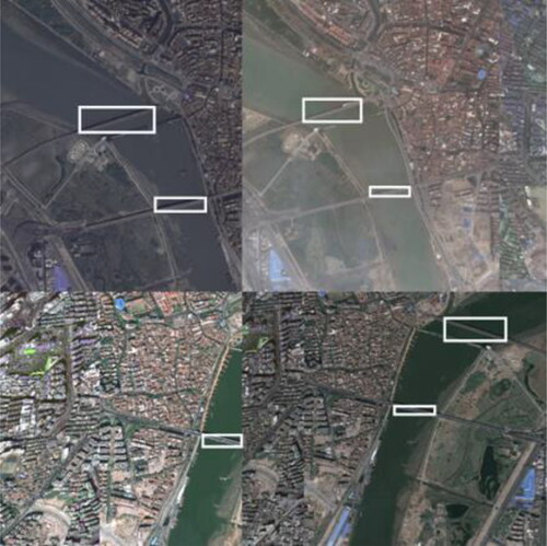
(3) Experiment on multiscale bridge detection in a large format image

The detection results on multiscale bridges in large format VHR shown in Figure 16. There are two missed detections in Centernet and YOLO-tiny, both of which can detect only the larger bridges under the image, and the accuracy of Centernet is low. Although YOLOv3, YOLOv4 and YOLO-lite can detect bridge objects with high precision, missed detection occurs, and the bridge under the image cannot be detected. This method can correctly detect all of the bridge objects. In addition, the F1 scores of single detected images are calculated according to Equations (13)–(15), and the methods (a), (b), (c), (d), (e), (f) are 0.50, 0.80, 0.80, 0.80, 0.50, 0.80, 1, respectively. The proposed method can balance Precision and Recall to achieve optimal detection results.

(4) Experiment on small-scale bridge detection

The experimental results on small-scale bridges are shown in Figure 16. YOLO-tiny has poor detection ability for small bridges, and only one bridge is detected. Centernet correctly detected 7 bridges with low accuracy, basically no more than 0.6. YOLO-Lite can detect 11 bridges, but the overall accuracy is not high, basically no more than 0.9. The proposed method has a similar effect compared with YOLOv3 and YOLOv4 in terms of detection ability and detection accuracy. It can detect bridges with high accuracy without false detection and missed detection.

(5) Experiment on large aspect ratio bridge detection

The detection results on bridges with large aspect ratios are shown in Figure 17. Centernet only correctly detected two bridges, there was one missing detection, and the accuracy of the correctly detected bridge was not high. YOLOv3 successfully and accurately detected three bridges, but the object bounding box range of the long bridge on the right side was not good and failed to frame the whole bridge. YOLOv4 has a good detection effect on the left and right bridges, but there is a false detection phenomenon in the middle bridge. We repeated the detection of a bridge object twice. YOLO-tiny has a good detection effect for the two bridges on the right, but there is repeated detection on the left. YOLO-lite can successfully detect three bridge objects, but the overall accuracy is not high. The accuracy of the two bridges on the left is only approximately 0.7. Compared with the other five methods, this proposed method has the best detection ability and detection effect.

(6) Experiment of cross-island bridge detection

The detection results on cross-island bridges are shown in Figure 18. Centernet and YOLO-Lite can accurately detect bridges, but the accuracy should be improved. Three bridges were detected by YOLOv3, but they were all false detections. The situation of YOLOv4 was the same, and two false detections occurred. YOLO-tiny also detected three bridges, including one false detection and one repeated detection. The definition of cross-island bridges in most bridge detection methods is not sufficiently clear, and the detection of cross-island bridges is easily disturbed by land in water areas. The proposed method has no false detection or missed detection and can detect bridges in images with high precision.

Through the above six groups of comparative experiments, the detection accuracy of the proposed method is significantly improved compared with the Centernet network with comparable speed. Compared with YOLOv3 and YOLOv4, the detection speed is greatly improved when the detection precision is slightly improved. For YOLO-tiny and YOLO-Lite, which are both lightweight networks, not only was the detection accuracy improved but also the bridge detection in complex scenes can be well handled. In summary, it was verified that the proposed method has a strong generalization ability for bridge detection in a variety of complex scenarios, and it is ahead of the current mainstream object detection methods in terms of detection speed and detection accuracy, which allows it to achieve both balance and optimization of speed and accuracy.

Next, experiments are conducted with the second bridge dataset. Since the background, scene, and shape of the bridge in this dataset are simpler compared to the first dataset, the detection results are not visualized for the individual images. Table 3 shows the results of the training bridge datasets using 8 object detection algorithms and the proposed method. From Table 3, it can be seen that all methods have different degrees of improvement for bridge detection in this dataset compared to the first dataset, which shows that the dataset has some influence on the performance impact of the bridge detection network. In this dataset, mAP, Precision, and F1 of the proposed method are optimal, and Recall and FPS are suboptimal, which verifies the robustness of the proposed method.

Table 3. Analysis of the main object detection algorithm results in the bridge dataset 2.

Method	mAP (%)	Precision (%)	Recall (%)	F1-score	FPS
Efficientdet	94.25	95.39	88.51	0.92	13.35
Retinanet	94.50	92.76	90.88	0.92	21.80
Centernet	93.11	96.86	83.33	0.90	47.44
YOLOv3	96.61	95.84	96.06	0.96	33.38
YOLOv4	91.94	92.95	92.00	0.92	23.67
YOLO-tiny	91.22	88.12	87.73	0.88	108.38
YOLO-lite	95.02	95.88	94.37	0.95	37.62
ASFF-YOLOv5	97.40	94.10	97.30	0.96	88.50
Proposed	97.62	97.11	94.71	0.96	73.62

5. Discussion

Through the multiple comparison experiments in Chapter 3, we obtained the following findings:

1. For faster bridge detection networks, such as Centernet, YOLO-lite, and YOLO-tiny, which are both lightweight and non-lightweight, the detection accuracy is lower than for slower bridge detection networks such as YOLOv3 and YOLOv4, and the detection capability is poor for most nonconventional bridges. Therefore, compressing only the backbone extraction feature network or increasing the speed of the bridge detection network only by means of parameter reduction will result in a significant loss in the detection precision and cannot achieve efficient and high-precision detection. In this paper, the bridge detection method has the advantages of both high accuracy and high time efficiency, and it is verified that the feature extraction network can be built by using depthwise separable convolution to maximize the feature extraction capability without changing the network structure and the number of effective convolution layers. The feature extraction and fusion capability can be further enhanced by combining a multiscale feature fusion pyramid and multibranch parallel dilated convolution.

2. In the multiscale bridge detection experiments, all of the methods could successfully detect large-scale bridges, but Centernet, YOLOv3, YOLO-lite, and YOLO-tiny failed to detect small-scale bridges. The method of YOLOv4 and this paper can detect both large-scale bridges and all small-scale bridges in the image, i.e. they have the capability of multiscale bridge detection. Therefore, the key point to achieve multiscale bridge detection is to ensure the detection effect for large-scale bridges while improving the detection capability for small-scale bridges as much as possible, which can be effectively solved by obtaining multiscale receptive fields and superimposing different receptive fields.

3. For large-format VHR bridge detection, bridge object pixels account for a relatively small number of pixels due to their large size and complex background, i.e. there is a serious imbalance between positive and negative samples. The results of the comparative experiments in this paper show that YOLOv3, YOLOv4, YOLO-lite and the methods in this paper have better detection effects compared with Centernet and YOLO-tiny because the first four methods have feature fusion modules of different degrees, which indicates that performing feature fusion can effectively solve this problem. However, the accuracy of the method in this case is relatively low, because the large size of VHR contains more information and more complex backgrounds, which makes it difficult to achieve a comprehensive and accurate detection of bridge targets. This is the part to be focused on in the subsequent study.

4. In the cross-island bridge detection experiments, YOLOv3, YOLOv4, and YOLO-tiny all had different degrees of incorrect detection and missing detection problems, and Centernet and YOLO-lite had lower detection precision. The reason is that the feature extraction ability of the above bridge detection methods is weak, which can be interpreted as the CNN being limited by the receptive field in the process of feature extraction and only extracting the local features of the bridge, failing to combine the surrounding features or background information of the bridge for overall feature extraction. This circumstance leads to difficulties in detecting bridges after being segmented by islands.

5. Applying the method in this paper to different remote sensing image bridge datasets, all of them can achieve relatively good results and realize the balanced optimum of accuracy and speed. It shows that the proposed method has good robustness and universality.

6. Although the method in this paper has excellent performance compared with most mainstream object detection methods, there is still some room for improvement in more complex datasets (e.g. Dataset 1) compared with the object detection method specifically for remote sensing images (ASFF-YOLOv5).

6. Conclusions

To realize efficient and accurate bridge detection in VHR, a depthwise separable multiscale feature fusion network for bridge detection is proposed in this paper. The proposed method mainly designs three modules: the backbone feature extraction network built by depthwise separable convolution, multibranch parallel dilated convolution and a cross-level feature fusion pyramid. This method has only 10.8 (million) parameters, and the size is only 41.2 MB. It realizes an effective compression of the network, in dataset 1, the detection speed reaches 60.04 FPS, and it can perform real-time detection of bridges. The average detection accuracy is 94.26%, which is higher than mainstream object detection networks. In dataset 2, the proposed method also achieves excellent results. In addition, it has strong bridge detection ability and can address bridge detection tasks in multiple scenes, such as multiscale, large format and complex background. The comprehensive index is better than other bridge detection methods and has strong practicability. Follow-up work will continue to optimize the backbone feature extraction network to achieve faster and more accurate bridge detection.

Abbreviations
DSMFFNet	=	depthwise separable multiscale feature fusion network for bridge detection in very high resolution remote sensing images
mAP	=	mean average precision
FPS	=	frame per second
VHR	=	very high resolution remote sensing images
CNN	=	convolutional neural network
DSC-CSPDarknet53	=	depthwise separable convolution and CSPDarknet53
CBM	=	convolution + banch normalization + mish
CSPX	=	cross stage PartialX

Disclosure statement

No potential conflict of interest was reported by the authors.

Appendix A:

List of test results

Table

Figure 13	(a)0.68 (b)1.00 (c)1.00 (d)0.94 (e)0.81 (f)1.00
Figure 14	(a)0.81 (b)1.00 (c)0.77 0.58 0.60 0.55 (d)1.00 (e)0.93 (d)1.00 0.95 0.83 0.66
Figure 15	(a)0.83 (b)0.68 0.96 (c)0.98 1.00 (d)0.95 (e)0.97 1.00 (f)0.69 0.54 0.94
Figure 16	(a)0.51 0.54 0.67 0.54 0.56 0.51 0.56 (b)1.00 1.00 1.00 1.00 1.00 1.00 1.00 0.99 0.99 1.00 0.98 (c)1.00 1.00 1.00 1.00 1.00 1.00 1.00 1.00 1.00 1.00 0.96 (d)0.88 (e)0.92 0.90 0.82 0.90 0.91 0.89 0.82 0.84 0.85 0.72 0.67 (f)0.99 1.00 1.00 0.98 0.92 1.00 1.00 0.99 0.93 0.98 0.90
Figure 17	(a)0.62 0.68 (b)0.99 0.99 0.89 (c)1.00 0.71 1.00 1.00 (d)0.71 0.84 0.80 0.97 (e)0.73 0.64 0.90 (f)1.00 1.00 1.00
Figure 18	(a)0.64 (b)1.00 0.74 0.66 (c)1.00 0.88 (d)0.90 0.59 0.62 (e)0.88 (f)1.00

Appendix B:

List of acronyms

Table

Acronyms	Full name
DSMFFNet	Depthwise Separable Multiscale Feature Fusion Network for Bridge Detection in Very High Resolution Remote Sensing Images
mAP	mean average precision
FPS	frame per second
VHR	Very High Resolution Remote Sensing Images
CNN	convolutional neural network
DSC-CSPDarknet53	depthwise separable convolution and CSPDarknet53
CBM	Convolution + Banch Normalization + Mish
CSPX	Cross Stage PartialX

References

- Bochkovskiy A, Wang C-Y, Liao H-YM. 2020. Yolov4: optimal speed and accuracy of object detection. arXiv Preprint arXiv:2004.10934.
- Cao Y, Wang Y, Peng J, Zhang L, Xu L, Yan K, Li L. 2020. DML-GANR: deep metric learning with generative adversarial network regularization for high spatial resolution remote sensing image retrieval. IEEE Trans Geosci Remote Sens. 58(12):8888–8904.
- Chaudhuri D, Samal A. 2008. An automatic bridge detection technique for multispectral images. IEEE Trans Geosci Remote Sens. 46(9):2720–2727.
- Chen L, Weng T, Xing J, Pan Z, Yuan Z, Xing X, Zhang P. 2020. A new deep learning network for automatic bridge detection from SAR images based on balanced and attention mechanism. Remote Sens. 12(3):441.
- Chen LC, Papandreou G, Kokkinos I, Murphy K, Yuille AL. 2018. DeepLab: semantic image segmentation with deep convolutional nets, atrous convolution, and fully connected CRFs. IEEE Trans Pattern Anal Mach Intell. 40(4):834–848.
- Dai J, Li Y, He K, et al. 2016. R-FCN: object detection via region-based fully convolutional networks. Neural Information Processing Systems. p. 379–387.
- Dalal N, Triggs B. 2005. Histograms of oriented gradients for human detection. 2005 IEEE Computer Society Conference on Computer Vision and Pattern Recognition. p. 886–893.
- Fan LS, Yang J, Peng YN. 2006. Feature extraction and target detection in river region based on cross entropy. J Syst Eng Electron. 03:339–341.
- Gaofen Challenge on Automated High-Resolution Earth Observation Image Interpretation 2020. [accessed]. http://en.sw.ch-reos.org.
- Girshick R, Donahue J, Darrell T. 2014. Rich feature hierarchies for accurate object detection and semantic segmentation. IEEE Conference on Computer Vision and Pattern Recognition(CVPR); Jun 23–28; Columbus, OH, USA.
- Girshick R. 2015. Fast R-CNN. IEEE International Conference on Computer Vision (ICCV); Dec 7–13; Santiago, Chile.
- He K, Zhang X, Ren S, Sun J. 2015. Spatial pyramid pooling in deep convolutional networks for visual recognition. IEEE Trans Pattern Anal Mach Intell. 37(9):1904–1916.
- He K, Zhang X, Ren S, Sun J. 2016. Deep residual learning for image recognition. IEEE Conference on Computer Vision and Pattern Recognition (CVPR), Las Vegas, Nevada, Jun 26–Jul 1.
- Howard AG, Zhu M, Chen B, Kalenichenko D, Wang W, Weyand T, Andreetto M, Adam H. 2017. MobileNets: efficient convolutional neural networks for mobile vision applications. arXiv Preprint arXiv: 1704.04861.
- Huang R, Pedoeem J, Chen, C. 2018. A real-time object detection algorithm optimized for non-GPU computers. 2018 IEEE International Conference on Big Data (Big Data); Dec 10–13; Seattle, WA.
- Jiang YM, Liu W, Lei L. 2006. Fusion model for bridge automatic detection in multi-source remote sensing imagery. J Electron Inf Technol. 10:1794–1797.
- Lin TY, Doll’ar P, Girshick RB, et al. 2017. Feature pyramid networks for object detection. CVPR. 1(2):4.
- Lin TY, Goyal P, Girshick R, He K, Dollár P. 2017. Focal loss for dense object detection. IEEE Trans Pattern Anal Mach Intell. 42(2):318–327.
- Liu S, Di H, Wang Y. 2017. Receptive field block net for accurate and fast object detection. Lect Notes Comput Sci. 11215:404–419.
- Liu W, Anguelov D, Erhan, D, Ssd. 2016. Single shot multibox detector. European Conference on Computer Vision; (ECCV); Oct 8–16; Amsterdam, Netherlands.
- Liu Y. 2020. Dense multiscale feature fusion pyramid networks for object detection in UAV-captured images. arXiv Preprint arXiv: 2012.10643.
- Lowe DG. 2004. Distinctive image features from scale-invariant key points. Int J Comput Vis. 60(2):91–110.
- Luo W, Li Y, Urtasun R, Zemel R. 2017. Understanding the effective receptive field in deep convolutional neural networks. 30th Conference on Neural Information Processing Systems (NIPS); Dec 4–9; Barcelona, Spain.
- Misra D. 2019. Mish: a self regularized non-monotonic neural activation function. arXiv Preprint arXiv: 1908.08681.
- Papageorgiou CP, Oren M, Poggio T. 1998. A general framework for object detection. The 6th IEEE International Conference on Computer Vision; Bombay, India.p. 555–562.
- Qiu ML, Huang L, Tang BH. 2022. ASFF-YOLOv5: multielement detection method for road traffic in UAV images based on multiscale feature fusion. Remote Sens. 14(14):3498.
- Redmon J, Divvala S, Girshick R, et al. 2015. You only look once: unified, real-time object detectiono. Proceedings of CVPR 2015. p. 779–788.
- Redmon J, Farhadi A. 2017. YOLO9000: better, faster, stronger. 2017 IEEE Conference on Computer Vision and Pattern Recognition (CVPR); Jul 21–26; Honolulu, HI, USA.
- Redmon J, Farhadi A. 2018. YOLOv3: an incremental improvement. arXiv Preprint arXiv 1804.02767.
- Redmon J, Farhadi A. 2018. YOLOv3: an incremental improvement. Computer Science – Computer Vision and Pattern Recognition, arXiv Preprint arXiv: 1804.02767.
- Ren S, He K, Girshick R, Sun J. 2017. Faster R-CNN: towards real-time object detection with region proposal networks. IEEE Trans Pattern Anal Mach Intell. 39(6):1137–1149.
- Ioffe S, Szegedy C. 2015. Batch normalization accelerating deep network training by reducing internal covariate shift. [accessed] https://arxiv.org/abs/1502.03167.
- Sermanet P, Eigen D, Zhang X, et al. 2013. OverFeat: integrated recognition, localization and detection using convolutional networks. IEICE Trans Fundam Electron Commun Comput Sci. arXiv Preprint arXiv: 1312.6229.
- Shi C, Zhang W, Duan C, Chen H. 2021. A pooling-based feature pyramid network for salient object detection. Image Vis Comput. 107(9):104099.
- Sithole G, Vosselman G. 2006. Bridge detection in airborne laser scanner data. ISPRS J Photogram Remote Sens. 61(1):33–46.
- Sun Y, Huang L, Zhao J, Change J, Chen P, Cheng F. 2022. High spatial resolution automatic detection of bridges with high spatial resolution remote sensing images based on random erasure and YOLOv4. Remote Sens Nat Resour. 34(02):97–104. (Chinese)
- Szegedy C, Ioffe S, Vanhoucke V, Alemi A. 2016. Inception-v4, Inception-ResNet and the impact of residual connections on learning. 31st AAAI Conference on Artificial Intelligence; Feb 4–9; San Francisco, CA
- Szegedy C, Wei L, Jia Y. 2015. Going deeper with convolutions. 2015 IEEE Conference on Computer Vision and Pattern Recognition (CVPR); Jun 9–12; Boston, MA.
- Takahashi N, Mitsufuji Y. 2020. Densely connected multidilated convolutional networks for dense prediction tasks. arXiv Preprint arXiv:2011.11844.
- Tan M, Pang R, Le QV. 2020. EfficientDet: scalable and efficient object detection. 2020 IEEE/CVF Conference on Computer Vision and Pattern Recognition (CVPR); Jun 13–19; Sattle, WA, USA.
- Tarhan C, Akar GB. 2018. Convolutional neural networks analyzed via inverse problem theory and sparse representations. IET Signal Proc. 13:219–223.
- Tong K, Wu Y, Zhou F. 2020. Recent advances in small object detection based on deep learning: a review. Image Vis Comput. 97:103910.
- Viola P, Jones M. 2004. Robust real-time face detection. Int J Comput Vis. 57(2):137–154.
- Wang CY, Liao H, Wu YH. 2020. CSPNet: a new backbone that can enhance learning capability of CNN. IEEE/CVF Conference on Computer Vision and Pattern Recognition Workshops (CVPRW); Jun 13–19; Seattle, USA.
- Xu D, Wu Y. 2021. FE-YOLO: a feature enhancement network for remote sensing target detection. Remote Sens. 13(7):1311.
- Yao X, Feng X, Han J, Cheng G, Guo L. 2021. Automatic weakly supervised object detection from high spatial resolution remote sensing images via dynamic curriculum learning. IEEE Trans Geosci Remote Sens. 59(1):675–685.
- Yu J, Zhou G, Zhou S, Yin J. 2021. A lightweight fully convolutional neural network for SAR automatic target recognition. Remote Sens. 13(15):3029.
- Yu X, Long W, Li Y, Shi X, Gao L. 2021. Improving the performance of convolutional neural networks by fusing low-level features with different scales in the preceding stage. IEEE Access. 9:70273–70285.
- Zhang X, Cao S, Chen C. 2020. Scale-aware hierarchical detection network for pedestrian detection. IEEE Access. 8:94429–94439.
- Zhang Y, Yuan Y, Feng Y, Lu X. 2019. Hierarchical and robust convolutional neural network for very high-resolution remote sensing object detection. IEEE Trans Geosci Remote Sens. 57(8):5535–5548.
- Zheng H, Wu Y, Deng L, Hu Y, Li G. 2020. Going deeper with directly-trained larger spiking neural networks. arXiv Preprint arXiv: 2011.05280.
- Zhou X, Wang D, Krhenbühl P. 2019. Objects as points. arXiv Preprint arXiv:1904.07850.
- Zhou X. 2020. Research on remote sensing image target detection Algorithm based on deep learning [MA dissertation]. Changsha University of Science and Technology. (Chinese).
- Zhu Y, Mu J, Pu H, Shu B. 2018. FRFB: integrate receptive field block into feature fusion net for single shot multibox detector. International Conference on Semantics Knowledge and Grids; Sep 12–14; Guangzhou, China. p. 173–180.
- Zou Z, Shi Z, Guo Y, Ye J. 2019. Object detection in 20 years: a survey. arXiv Preprint arXiv: 1905.05055v2.