Testing Sentinel-2 spectral configurations for estimating relevant crop biophysical and biochemical parameters for precision agriculture using tree-based and kernel-based algorithms

Abstract

Sentinel-2 spectral configurations, S2-10m and S2-20m, were evaluated for retrieving essential crop biophysical and biochemical parameters and their effect on the performance of three machine learning regression algorithms (MLRAs) in two African semi-arid sites. The results were benchmarked against all spectral bands (S2-All). The results show that the S2-20m was more robust in retrieving Leaf Area Index (LAI) (RMSE_cv: 0.58 m² m⁻², 0.47 m² m⁻²), while the S2-10m provided optimal retrievals Leaf Chlorophyll a + b (LC_ab) (RMSE_cv: 6.89 µg cm⁻², 7.02 µg cm⁻²) for the two sites, respectively. In contrast, S2-20m performed better in retrieving Canopy Chlorophyll Content (CCC) in Bothaville to an RMSE_cv of 35.65 µg cm⁻², while S2-10m yielded relatively lower uncertainties (RMSE_cv of 26.84 µg cm⁻²) in Harrismith. Moreover, various MLRAs were sensitive to the various spectral configurations, and performance varied by site. GPR and XGBoost were more robust, and thus have the most potential for crop biophysical and biochemical parameter retrieval in both sites. Based on the benchmark results, the two configurations can be used independently. The results obtained here are relevant for the rapid development of essential crop biophysical and biochemical parameters for precision agriculture using Sentinel-2’s 10 m or 20 m bands, without the need for resampling.

Keywords:

• Crop biophysical parameters
• Sentinel-2
• Random Forest
• eXtreme Gradient Boosting
• Gaussian process regression

Introduction

Food and nutrition security improvement has been the principal mandate for every nation within the Sustainable Development Goals (SDGs) framework for alleviating hunger and poverty in the light of population growth (Mango et al. 2017), with the most significant growth constituted by developing countries (Walker 2016). These countries are currently affected by a marginal mismatch between the demand for food and agricultural production (Godfray and Garnett 2014). For instance, southern Africa is facing massive urbanization, income, and population growth which are constantly and increasingly hurling up the demand for food and emerging challenges presented by climate change and natural resources constraints. Meanwhile, agriculture is still the mainstay of many economies in southern Africa contributing a gross domestic product of 35%, employing between 70% and 80%, and producing ∼30% of foreign exchange while also sustaining about 70% of the smallholder farmers’ livelihoods (Mango et al. 2017). Although South Africa produces surplus food, household and individual food insecurities are still glaring especially in the rural communities. The agricultural sector plays an invaluable role, and therefore, the sector needs to be optimised to bridge the gap between national and household food insecurities. There is a need for time-efficient monitoring frameworks grounded on spatially explicit technologies for near real-time monitoring of crop production indicators. Crop production indicators and attributes include the extent of cropland, irrigated cropland, crop structure and growth parameters (i.e. chlorophyll, leaf area index, biomass) and yield (Delegido et al. 2011).

Traditional in-situ, lab-based and empirical point-based sampling techniques have been used to assess crop productivity. These field-based techniques are highly accurate. However, they are laborious, time-consuming, and inadequate in spatially and temporally characterising plant productivity. Therefore, they are not suitable for assessing expansive croplands. Remote sensing has emerged mainly as a non-invasive, resource-efficient method of monitoring crop productivity elements through time and space in a spatially-explicit manner (Lawley et al. 2016). Specifically, the premise of monitoring crops using remotely sensed data is based on the spectral signatures or properties of crops which tend to vary with growth stage, health state and type of crop. Through time, remote sensing of crops has developed from airborne systems in the 1970s (Maxwell 1976; Collins 1978) to more sophisticated satellite-based sensors such as Landsat, which offered an efficient means to repeatedly monitor agricultural crop productivity at larger scales. Although Landsat missions have been successfully used to estimate crop productivity elements in previous studies (Gitelson et al. 2012; Gao et al. 2017; Ma et al. 2018; Croft et al. 2020), these sensors do not cover all the critical sections such as red-edge section of the electromagnetic spectrum that is instrumental in characterising crop productivity and widely associated with chlorophyll content and Leaf Area Index (LAI) variability (Chemura et al. 2017). In the recent past, the earth observation community witnessed the launching of the Sentinel-2 Multi-Spectral Instrument (MSI) closes this gap, making it more suitable for crop productivity elements mapping.

The MSI sensors onboard Sentinel-2 2 A and 2B satellites provide 13 spectral bands covering the visible (VIS), red-edge (RE), near-infrared (NIR), and shortwave infrared (SWIR) spectrums. Their revisit frequency of 5 days and the spatial resolutions of 10 m and 20 m present better prospects in crop biophysical and biochemical retrieval (Delegido et al. 2011). The traditional broad (i.e. 30–115 nm) VNIR bands are available at 10 m (S2-10m), while the strategically-located narrow (15–20 nm) RE and NIR bands, as well as SWIR bands have 20 m resolution (S2-20m). In this regard, data fusion techniques such as Super-Resolution for Multispectral Multiresolution Estimation (SupReMe) (Lanaras et al. 2017) and DSen2 (Lanaras et al. 2018) have been proposed for improving the spatial resolution of S2-20m bands to match the relatively high resolution of S2-10m without compromising the spectral consistency. Although the highest spatial resolution is often desired, Kganyago et al. (2020) show that the difference in LAI accuracy between Sentinel-2 MSI bands resampled to 10 m and 20 m spatial resolutions is negligible. Nonetheless, the spatial resolutions of up to 20 m, are regarded as sufficient for precision agriculture applications (Mulla 2013).

While numerous studies show that LAI, Leaf Chlorophyll Content (LC_ab) and Canopy Chlorophyll Content (CCC) can be retrieved with the entire spectral coverage of Sentinel-2 MSI (Xie et al. 2019; da Silva et al. 2020; Kobayashi et al. 2020; Segarra et al. 2020), others (Delegido et al. 2013; Verrelst et al. 2016; Clevers et al. 2017) show that only a few bands are necessary for achieving high accuracies. Clevers et al. (2017), for example, found that vegetation indices constructed using S2-10m (i.e. VNIR) were better at retrieving LAI, LC_ab, and CCC of Potato crops, while Delegido et al. (2013) found that the exclusion of S2-20m RE bands resulted in systematic errors in the retrieval of LAI and CCC for multiple crops with simulated Sentinel-2 data. In other studies, (Verrelst et al. 2015; Chrysafis et al. 2020; Kganyago et al. 2021) Sentinel-2 SWIR bands were identified among the most influential variables in various machine learning models for LAI, LC_ab, and CCC retrieval. Therefore, it is essential to evaluate the individual performance of the different sentinel-2 spectral configurations at 10 m, i.e. characterised by broad VNIR bands (hereafter, S2-10m), and 20 m, i.e. characterised by RE-NIR-SWIR bands (hereafter, S2-20m) spectral bands in biophysical and biochemical parameter retrieval to demystify these inconsistencies. This is a worthy endeavour especially since various biophysical and biochemical traits affect the various regions of the electromagnetic spectrum differently.

Meanwhile, the literature also underscores the importance of Machine Learning Regression Algorithms (MLRAs) in building models for characterising the spatial distribution of crop productivity elements. Generally, MLRAs are categorised into three according to their architectural designs, i.e. tree-based or tree ensembles (e.g. Random Forest, RF), kernel-based (e.g. Support Vector Machines, SVM), and deep learning (e.g. Artifical Neural Networks, ANN) (Rivera-Caicedo et al. 2017). Among these, tree-based and kernel-based MLRAs are often applied for estimating crop BVs in previous studies because they are relatively less complicated, computationally fast, have good accuracy and require relatively few intuitive hyperparameters when compared to deep learning MLRAs (Wang et al. 2018; Shah et al. 2019; Kganyago et al. 2021). For example, (LI et al. 2017) found R² of 88% and an RMSE of 0.195 m² m⁻² in retrieving grassland LAI using RF, and Landsat Enhanced Thematic Mapper (TM+) and operational Land Imager (OLI) data. Others (Camps-Vails et al. 2009; Verrelst et al. 2011, 2012, 2013, 2016; Camacho et al. 2021) show that kernel-based algorithms such as Gaussian Regression Process (GPR) outperform other popular algorithms of the same family such as SVM and Kernel Ridge Regression (KRR) as well as ANN and therefore offer better prospects for biophysical and biochemical retrieval due to its superior accuracy and unique capability to provide uncertainty estimates of the response variable. These uncertainty estimates allow the assessment of the robustness of the retrievals for operational applications. Despite the optimal performance of these MLRAs, the literature also states that no algorithm is suitable for all contexts (Ndlovu et al. 2021). Thus, their performance varies by crop conditions and types, environments and sensors (according to their spectral and spatial configurations) (Delloye et al. 2018). Related studies (Delloye et al. 2018; Verrelst et al. 2012) were conducted in the Temperate maritime and Mediterranean climate, using simulated data, and compared complex, unexplainable, i.e. ‘black box’, algorithms such as ANN and Kernel Ridge Regression (KRR). In this regard, there is still a need to compare and identify relevant and effective algorithms (including less complex, robust and explainable algorithms) for specific contexts such as crop biophysical and biochemical parameters retrieval in semi-arid environments. Therefore, the objectives of this study were: (1) to evaluate the performance of the Sentinel-2 spectral configurations, i.e. S2-10m (VNIR), and S2-20m (RE-NIR-SWIR), benchmarked against all spectral bands (S2-All), in estimating crop biophysical and biochemical parameters; and (2) to determine the effect of Sentinel-2 spectral configurations on the performance of three MLRAs, i.e. Random Forest (RF), eXtreme Gradient Boosting (XGBoost), and Gaussian Process Regression (GPR), in retrieving LAI, LC_ab and CCC. These MLRAs were chosen based on their competitive accuracy achieved in previous studies as well as well as other advantages such as their robustness, low complexity, and require only a few hyperparameters (Verrelst et al. 2015, 2016; Rivera-Caicedo et al. 2017; Estévez et al. 2020; Mansaray et al. 2020; Pathy et al. 2020; Amin et al. 2021; Kganyago et al. 2021). The study was conducted over Maize (Zea mays L.), Beans (Phaseolus vulgaris), and Peanuts (Arachis hypogaea L) characterised by contrasting physiological pathways, leaf and canopy structures and architectures, thus offering generic models that may be widely applicable. The generic models are critical in African contexts where intercropping and mixed crop management practices are dominant. The contribution of this study is in elucidating the optimal Sentinel-2 configuration and MLRA combinations for estimating specific crop BVs in semi-arid areas. The results could inform future satellite-based product development and operational solutions for precision agriculture.

Materials and methods

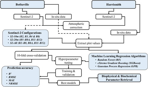
The flowchart summarising the methods followed in the current study is presented in Figure 1.

Figure 1. Summary of the methods followed in the study.

Experimental sites

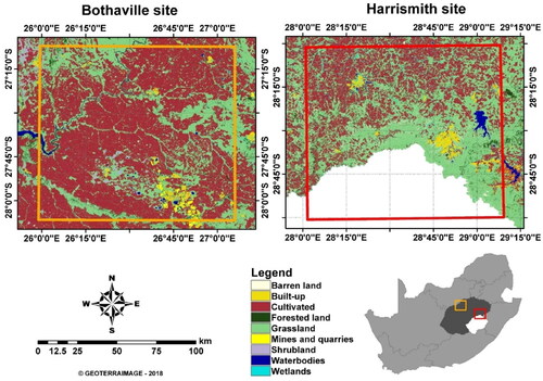
This study was conducted in two experimental sites located in Bothaville and Harrismith in Free State province, South Africa (Figure 2). The experimental sites are situated in the main agricultural production zone of the country, i.e. Free State, with more 3 million Ha of land cultivated. Bothaville—used as a test site in this study—is located at latitudes: 27°13′0ʺS to 28°8′0ʺS, and longitudes: 26°0′0ʺE to 27°05′0ʺE, while Harrismith—used as a validation site in this study—borders Lesotho in the South via Drakensberg Mountains and is located at latitudes: 28°0′0ʺS to 29°0′0ʺS and longitudes: 28°0′0ʺE to 29°8′0ʺE. The two-experience warm and wet summers, with mean temperatures of ∼18 °C and ∼19.2 °C and annual mean rainfall of ∼584 mm and 115 mm, respectively. The summer season represents the main cropping season (i.e. from December to May or June). Free State province is dominated by medium- to large-scale commercial farming, with an average field size of 2 336 Ha (http://www.ard.fs.gov.za/wp-content/uploads/2019/10/APP-FINAL-2019-22.pdf), where the typical main crops are Maize, Sunflower, and Groundnuts in Bothaville and Maize, Soybeans, and Dry beans in Harrismith. The crops in Bothaville are grown on sandy to sandy-loamy soils on generally flat slopes, while Harrismith soils are clay-loamy with higher water-retention capacities on undulating slopes.

Figure 2. Land cover types and locations of Bothaville (orange), and Harrismith (red), in Free State province (dark grey), South Africa. Study area map adopted from Kganyago et al. (2021).

Data

In-situ data

The in-situ LAI and LC_ab and CCC data were collected in the field from 15th to 26th of March 2021 in Harrismith and from 11th to 23rd of April 2021 in Bothaville. LAI and LC_ab measurements were collected non-destructively within 40 m × 40 m plots, selected along randomly transects. Trimble® TDC600 handheld Data Collector, with global navigation satellite systems (GNSS) accuracy of 1.5 m, was used to Geo-tag the centroid of each plot and take plot pictures. Each plot consisted of an average of six to eight random measurements for each of the main crops at each site, i.e. Maize (Zea mays L.), Beans (Phaseolus vulgaris), Peanuts (Arachis hypogaea L) in Bothaville and Maize and Beans in Harrismith. These crop types, therefore, allowed the development of generic MLRA models (i.e. with a potential for wide application) since they have contrasting physiological pathways, leaf and canopy structures and architectures. For LAI measurements, we used LiCor 2200c Plant Canopy Analyzer (Li-Cor, Inc., Lincoln, NE, USA) in both field campaigns, with a 180° view cap to shield the influence of the operator and unequal sky conditions on the measurements. In contrast, LC_ab measurements were an internal average of eight to nine sun-exposed leaves at each sampling point and were collected with MC-100 Chlorophyll Concentration Meter (Apogee Instruments, Inc., Logan, UT, USA). The MC-100 is calibrated to measure chlorophyll concentration in absolute units, i.e. µmol m⁻², achieved through crop-specific and generic calibration coefficients which are applied to the measured ratio of transmission at 931 nm to 653 nm (Parry et al. 2014). To be consistent with previous studies, the chlorophyll concentration values in µmol m⁻² were converted to µg cm⁻². The canopy chlorophyll content (CCC) for each plot was estimated as a product of LC_ab and LAI (LC_ab × LAI) (Jacquemoud et al. 2009). Since our aim was not to develop crop-specific biophysical and biochemical parameters retrieval models, the field data for all crops found at each site were combined. The descriptive statistics of the field data in Bothaville and Harrismith are displayed in Table 1.

Table 1. Descriptive statistics of measured LAI (m² m⁻²), LC_ab (µg cm⁻²) and CCC (µg cm⁻²) at the two sites.

	Bothaville					Harrismith
	n	Min	Mean	Max	SD	n	Min	Mean	Max	SD
LAI	172	1.78	3.37	5.75	0.90	179	1.16	3.54	6.17	0.88
LCab	172	3.32	29.09	63.62	14.75	179	10.77	27.71	56.83	10.57
CCC	172	7.87	104.25	339.09	71.23	179	20.44	96.81	282.54	43.68

Remotely sensed data

Sentinel Hub Cloud API for Satellite Imagery (Sinergise Laboratory for geographical information systems, Ltd., Ljubljana, Slovenia) was used to retrieve the Sentinel-2 Multi-Spectral Imager (MSI) reflectance image (granule: 35JMK), acquired on the 14th of April 2021 over Bothaville and 22nd of March 2021 (granule: 35JPJ) over Harrismith. These acquisition dates coincided with the dates of field data collection at each experimental site. Sentinel-2A and 2B conjunctively provide a 5-days revisit period and carry the identical MSI sensors. MSI sensors acquire images in 13 bands at 10 m (i.e. Band 2:490 nm, Band 3:560 nm, Band 4:665 nm, and Band 8:842 nm), 20 m (i.e. Band 5:705 nm, Band 6:740 nm, Band 7:783 nm, Band 8 A:865 nm, Band 11:1610 nm, and Band 12:2190 nm), and 60 m (i.e. Band 1:443 nm, Band 9:945 nm, and band 10:1375 nm) spatial resolution. The bands at 60 m were dedicated for atmospheric correction and cloud screening using Sen2cor (Drusch et al. 2012). Sen2cor is a Sentinel-2 dedicated atmospheric correction (including cirrus clouds and terrain correction) processor. The algorithm uses the libRadtran database of look-up tables (LUTs) generated for a wide variety of atmospheric conditions, solar geometries, and ground elevations to convert the Level-1C Top-of-Atmosphere (TOA) image data to Bottom-of-Atmosphere (BOA) reflectance. The image data was corrected using parameters: atmospheric model ‘Mid-latitude summer’, aerosol type ‘Rural’ and two-band water volume retrieval (i.e. 940 nm and 1130 nm). Further details on Sen2Cor can be obtained from Mueller-Wilm (2016) and Louis et al. (2016). For further analysis, the spectral bands were grouped according to their native spatial resolutions, i.e. S2-10m (i.e. B2, B3, B4, and B8) and S2-20m (i.e. B5, B6, B7, B8A, B11, and B12). S2-All bands consisted of the 10 m bands and 20 m bands resampled bands to 10 m using the nearest neighbour resampling technique in SNAP software v8.0 (Sentinel Application Platform, http://step.esa.int) because of its ability to maintain the spectral fidelity of the data.

Crop and green-vegetation masking

A crop mask derived from the National Crop Boundaries Dataset (CropEstimatesConsortium 2017) was used to mask non-croplands on the Sentinel-2 bands. However, this dataset did not necessarily represent the active crop fields during the period of the current study (i.e. March and April 2021) since it is generated from SPOT 5 and 6 data acquired in 2014 and 2015. Therefore, a vegetation mask generated from the NDVI (calculated from each respective image), was used to mask non-vegetated pixels (i.e. those with NDVI < 0.2) from further analysis. This constrained further analysis to the planted crop fields in the 2021 summer growing season.

Machine learning regression algorithms

The MLRAs used in this study were chosen based on their good accuracy achieved in previous studies (Verrelst et al. 2015, 2016; Rivera-Caicedo et al. 2017; Estévez et al. 2020; Mansaray et al. 2020; Pathy et al. 2020; Amin et al. 2021; Kganyago et al. 2021).

Random Forest

Random Forest (Breiman 2001) is an ensemble tree-based machine learning algorithm for classification and regression and an improvement of Classification and Regression Trees (Breiman et al. 1984). In contrast to Classification and Regression Trees (CART), Random Forest (RF) uses bagging (or bootstrapping) to iteratively and independently build a large number of decision trees (ntree) based on a random subset of training samples created by resampling with replacement from the original sample (Fawagreh et al. 2014; Breiman 2001). Then, for each bootstrap sample, a decision tree is fit using randomly selected features (mtry), which are used to split each node in the tree (i.e. binary partitioning). Therefore, the trees grown from different and random subsets ensure increased diversity of decision trees and reduced bias of the regression (Pal 2005; Gislason et al. 2006; Rodriguez-Galiano et al. 2012). The final regression output is obtained as an average across all trees (Pal 2005; Gislason et al. 2006). The remaining training samples from each created random sample by bagging are called out-of-bag (OOB) data and are used for regression evaluation (Gislason et al. 2006). The optimal RF hyperparameters (i.e. mtry and ntree) for each configuration and response variable (i.e. LAI, LC_ab, and CCC) were tuned using the Grid-search strategy, and the optimal models were selected as those that have the lowest RMSEcv. The mtry ensures that the trees in the ensemble have low bias, high variance and are less correlated; and thus, preventing over-fitting (Loggenberg et al. 2018). On the other hand, while the prediction accuracy will generally improve with increasing ntree up to a certain point, previous studies show that this parameter has low impact on the accuracy and can be as high as possible (Du et al. 2015; Guan et al. 2013).

Extreme gradient boosting

Extreme Gradient Boosting (XGBoost) (Chen and Guestrin 2016) is an improved implementation of Gradient Boosting Machines (GBM), also known as Gradient Boosted Regression Trees (GBRT) (Friedman 2001), bringing several additional features and advantages. It uses gradient boosted decision trees and a more regularised formalisation to avoid over-fitting, handles missing values (or sparse data) more efficiently, employs parallel and distributed computing for rapid tree construction and building of large models, respectively, and can fit new data added to the trained model. Thus, XGBoost is computationally effective and often outperforms other algorithms (Chen and Guestrin 2016; Beltran et al. 2019). Provided with the training dataset containing predictor and response variables, XGBoost generally works as follows:

1. Sort the predictors and search for the optimal node splits,

2. Choose an optimal split from the predictor that optimizes the objective function, which consists of the loss function ($d$) and a regularisation term ($\beta$) (see Eq. (1)(1) $$\mathrm{\Omega }\left(\theta \right)=\sum _{i=1}^{n}d(y_i,{\widehat{y}}_i)+\sum _{k=1}^K\beta \left(f_k\right)$$(1) ).

(1) $$\mathrm{\Omega }\left(\theta \right)=\sum _{i=1}^{n}d(y_i,{\widehat{y}}_i)+\sum _{k=1}^K\beta \left(f_k\right)$$(1) where ${\widehat{y}}_i$ is the predictive value, $n$ is the number of instances in the training data, $K$ is the number of trees, $f_k$ is a tree from the ensemble of trees. In this study, the Mean Squared Error (MSE, Eq. (2)(2) $$\mathit{MSE}=(y_i-{\widehat{y}}_i^{(t-1)}{)}^2$$(2) ) was used as the loss function. (2) $$\mathit{MSE}=(y_i-{\widehat{y}}_i^{(t-1)}{)}^2$$(2)

• Repeat steps 1 and 2 until the most extreme tree depth is achieved,

• Assign the prediction scores to the leaves, and prune any negative nodes using a bottom-up approach,

• Repeat the above steps in a value adding manner until the predetermined number of iterations is reached.

The XGBoost algorithm requires parameterisation of several parameters, which include the following pertinent ones for the tree booster: learning rate (eta, shrinks the feature weights and prevents overfitting), maximum tree depth (max_depth, controls the complexity of the model where a higher value result in a complex and deep tree), minimum sum of instance weight (min_child_weight, controls the partitioning of trees below which further tree partitioning would terminate), sampling ratio per tree (subsample, helps to prevent overfitting), minimum loss reduction (gamma, controls further partitioning of the tree leaf nodes where the larger value will result in a conservative model), and L1 and L2 regularisation terms on weights (alpha and lambda, respectively). The optimal hyper-parameters were selected using the lowest Root Mean Squared Error of cross-validation (RMSE_cv) based on the 10-fold Cross Validation (CV) resampling strategy. We refer the interested readers to excellent mathematical descriptions of XGBoost, which can be found in the original publication, Chen and Guestrin (2016), and others (Ayumi 2017) and (Gupta et al. 2016).

Gaussian process regression

The Gaussian process regression (GPR) (Rasmussen 2003) is a kernel-based probabilistic approach that establishes a relation between explanatory variables (e.g. spectral bands) and the output variable (e.g. LAI). To infer an unknown functional relationship from a training dataset, GPR elicits a prior GPR to constrain the possible form of the unknown function. Then, it updates the prior GPR in the light of training samples to generate the posterior GPR as the final functional model (Williams and Rasmussen 2006). A scaled Gaussian kernel is commonly used, which required hyperparameters, signal $(v, {\sigma }_b)$ and noise ${\sigma }_n,$ i.e. $\theta =\{v, {\sigma }_b, {\sigma }_n\}.$ These hyper-parameters $\theta$ combats model overfitting and are typically selected by Type-II Maximum Likelihood, using the analytical marginal likelihood (also called evidence) of the observations (Verrelst et al. 2016). Often, the derivatives of the log-evidence are also analytical; thus, conjugated gradient ascent is typically used for optimisation (Camps-Vails et al. 2009). The GPR has recently gained popularity due to its competitive accuracy and capability to provide uncertainty estimates of the response variables (Camps-Vails et al. 2009; Verrelst et al. 2012a, 2013, 2016; Camacho et al. 2021). It was selected in the current study because of its high accuracy, robustness to overfitting and rapid training speeds. The GPR hyperparameters for this study were automatically optimised in ARTMO software (Available online: https://artmotoolbox.com/, accessed: 27 October 2021) based on the training data, using 10-fold CV, where the optimal combination of hyperparameters used for training the models was selected as the one that minimised the prediction error (RMSE_cv). For detailed account of GPR in remote sensing, we refer the reader(s) Camps-Valls et al. (2016) and others that applied it for biophysical and biochemical retrieval (Verrelst et al. 2012a, 2013; Delegido et al. 2015; Verrelst et al. 2015, 2016; Estévez et al. 2020; Amin et al. 2021).

Model training and validation

For training and validation, this study used k-fold cross-validation, i.e. k = 10 for this study, to ensure that all data are used for both training and validation instead of the traditional split into 70% training vs 30% validation (Snee 1977; Verrelst et al. 2015; Shah et al. 2019). Prior to model training and validation, average pixel values were extracted from the intersecting image pixels within plot blocks of 40 m × 40 m. During the k-fold cross-validation (cv), the dataset is randomly divided into equal k sub-datasets. Then, a training dataset is formed by k − 1 sub-datasets, while a validation dataset is formed by a one k sub-dataset. The final estimation value is a combination of the iterative validation steps, i.e. k times, using one of the k sub-datasets each time.

The prediction accuracies of each MLR model and the experimental scenario were assessed using 10-fold cross-validation (cv) with the coefficient of determination (R²), Root Mean Squared Error (RMSE), Mean Absolute Error (MAE), and Normalised RMSE (NRMSE) (Eqs. (1)–(4)) as recommended by Richter et al. (2012). (1) $$R^2=\mathrm{ }\frac{\sum (y_i^n-\mathrm{ }{\overline{y}}_i{)}^2}{\sum (y_i\mathrm{ }-{\overline{\mathrm{ }y}}_i{)}^2},$$(1) (2) $$\mathit{RMSE}=\mathrm{ }\sqrt{\frac{1}{n}\mathrm{ }\sum _{i=1}^n(x_i-y_i{)}^2\mathrm{ }},$$(2) (3) $$\mathit{MAE}=\mathrm{ }\frac{1}{n}\sum _{i=1}^n|x_i-y_i|,$$(3) (4) $$\mathit{NRMSE}=100\mathrm{ }\times \left(\frac{\mathit{RMSE}}{y_{\text{max }}-\mathrm{ }{y}_{\min }}\right),$$(4) where $y_i$ and ${\overline{y}}_i$ in Eq. (1)(1) $$\mathrm{\Omega }\left(\theta \right)=\sum _{i=1}^{n}d(y_i,{\widehat{y}}_i)+\sum _{k=1}^K\beta \left(f_k\right)$$(1) denote the biophysical or biochemical predictions and mean of the observed (or measured) biophysical or biochemical parameter (e.g. LC_ab), respectively, while x_i and y_i in Eqs. (2)–(3) denote the observed and predicted biophysical or biochemical parameter (e.g. LC_ab), respectively, and n is the number of samples. $y_{\text{max }}$ and $y_{\min }$ in Eq. (4)(4) $$\mathit{NRMSE}=100\mathrm{ }\times \left(\frac{\mathit{RMSE}}{y_{\text{max }}-\mathrm{ }{y}_{\min }}\right),$$(4) denote the maximum and minimum values of the observed values.

All model building, prediction accuracy assessment, and biophysical and biochemical parameter mapping were performed in MATLAB based software application, i.e. ARTMO version 3.29 (Available online: https://artmotoolbox.com/, accessed: 27 October 2021), using MLRA Toolbox (Camps-Valls et al. 2013).

Results

This study evaluated the performance of the various Sentinel-2 configurations, i.e. S2-10m (VNIR) and S2-20m (RE-NIR-SWIR), in estimating LAI, LC_ab, and CCC using three Machine learning regression algorithms, i.e. RF, XGBoost, and GPR. The resulting accuracies for each crop biophysical and biochemical parameter were benchmarked against all spectral bands (S2-All) resampled to 10 m—the highest spatial resolution available from Sentinel-2.

Crop biophysical and biochemical parameter retrieval accuracies using MSI configurations

The two Sentinel-2 MSI configurations, i.e. S2-10m and S2-20m, showed varying performances for different biophysical and biochemical parameters (Tables 2 and 3). For LAI, S2-20m resulted in consistently superior performance between the two sites, where the highest RMSE_cv of 0.58 and 0.47 m² m⁻² were achieved for Bothaville and Harrismith, respectively. Consistently, S2-20m explained the greatest variability, i.e. 58% and 72%, when compared to S2-10m, which explained only 52% and 64% for two sites, respectively. A benchmark against the full MSI spectral data (i.e. S2-All) indicated consistently similar performances with S2-20m between the two sites.

Table 2. The performance of S2-10m (VNIR), S2-20m (RE-NIR-SWIR), S2-All (all) spectral bands for estimating LAI (m² m⁻²), LCab (µg cm⁻²), and CCC (µg cm⁻²) with three MLRAs in Bothaville.

		S2-10m			S2-20m			S2-All
		RF	XGBoost	GPR	RF	XGBoost	GPR	RF	XGBoost	GPR
LAI	R2	0.52	0.52	0.52	0.58	0.57	0.54	0.55	0.59	0.52
	RMSEcv	0.62	0.63	0.62	0.58	0.59	0.61	0.60	0.58	0.63
	MAEcv	0.41	0.43	0.44	0.38	0.41	0.42	0.40	0.42	0.44
	NRMSEcv	15.72	15.78	15.66	14.80	14.93	15.44	15.22	14.67	15.75
LCab	R2	0.77	0.79	0.77	0.74	0.75	0.75	0.75	0.75	0.75
	RMSEcv	7.08	6.89	7.11	7.50	7.47	7.34	7.36	7.38	7.30
	MAEcv	5.48	5.40	5.46	5.66	5.66	5.53	5.51	5.63	5.61
	NRMSEcv	11.74	11.42	11.78	12.44	12.39	12.18	12.21	12.24	12.10
CCC	R2	0.69	0.73	0.70	0.74	0.76	0.70	0.73	0.74	0.72
	RMSEcv	39.57	37.66	38.92	36.54	35.65	39.17	36.88	36.84	37.67
	MAEcv	26.71	26.73	26.66	25.23	25.32	26.52	25.31	26.48	25.71
	NRMSEcv	11.95	11.37	11.75	11.03	10.76	11.83	11.14	11.12	11.37

The bold formatted numbers indicate the lowest RMSE_cv achieved for each biophysical and biochemical parameter and spectral configuration.

Table 3. The performance of S2-10m (VNIR), S2-20m (RE-NIR-SWIR), S2-All (all) spectral bands for estimating LAI (m² m⁻²), LCab (µg cm⁻²), and CCC (µg cm⁻²) with three MLRAs in Harrismith.

		S2-10m			S2-20m			S2-All
		RF	XGBoost	GPR	RF	XGBoost	GPR	RF	XGBoost	GPR
LAI	R^2	0.54	0.55	0.64	0.54	0.54	0.72	0.61	0.59	0.71
	RMSEcv	0.59	0.60	0.53	0.60	0.61	0.47	0.56	0.58	0.48
	MAEcv	0.45	0.47	0.40	0.39	0.46	0.31	0.43	0.45	0.32
	NRMSEcv	11.89	12.00	10.52	11.98	12.14	9.31	11.26	11.56	9.51
LCab	R^2	0.55	0.54	0.56	0.53	0.53	0.57	0.55	0.57	0.57
	RMSEcv	7.09	7.14	7.03	7.21	7.29	7.02	7.10	6.96	6.92
	MAEcv	5.53	5.50	5.48	5.63	5.69	5.32	5.48	5.37	5.29
	NRMSEcv	15.40	15.52	12.25	15.65	15.82	15.24	15.42	15.11	15.03
CCC	R^2	0.60	0.61	0.62	0.58	0.57	0.57	0.59	0.61	0.59
	RMSEcv	27.41	27.46	26.84	28.17	28.81	28.71	27.95	27.55	28.08
	MAEcv	20.12	20.44	19.93	20.93	21.44	20.85	20.99	20.64	20.62
	NRMSEcv	10.46	10.48	10.24	10.75	10.99	10.96	10.67	10.51	10.71

The bold formatted numbers indicate the lowest RMSE_cv achieved for each biophysical and biochemical parameter and spectral configuration.

The results for LC_ab (also shown in Tables 2 and 3) showed that S2-10m was superior to S2-20m in Bothaville, with RMSE_cv of 6.89 µg cm⁻² (R²: 0.79), while S2-20m only achieved RMSE_cv of 7.34 µg cm⁻² (R²: 0.75). However, in Harrismith, the two configurations resulted in equivalent retrieval accuracies, with RMSE_cv ≈ 7.0 µg cm⁻² (R² ≈ 0.55). When benchmarking S2-10m LC_ab results (in Bothaville) with S2-All, the results show that it outperforms S2-All, while in Harrismith, S2-All slightly outperformed both S2-10m and S2-20m. Lastly, S2-20m resulted in the most robust estimates of CCC in Bothaville, with RMSE_cv of 35.65 µg cm⁻² and explained 76% of CCC variability when compared to S2-10m (RMSE_cv: 37.66 µg cm⁻²; R²: 0.73). However, contradictory results were found in Harrismith, where S2-20m was relatively worse, achieving RMSE_cv of 28.17 µg cm⁻² (R²: 0.58) when compared to the relatively better estimates of S2-10m (RMSE_cv: 26.84 µg cm⁻²; R²: 0.62). The benchmarking (i.e. S2-All) results were worse than those obtained for Bothaville with S2-20m and Harrismith with S2-10m. Overall, both spectral configurations (i.e. S2-10m and S2-20m) also achieved NRMSE_cv of <20%, with the highest NRMSE_cv, i.e. ≈11%, being achieved for LAI and CCC in Bothaville, and all biophysical and biochemical parameters in Harrismith.

Comparison of MLRAs accuracies under various spectral configurations

The three MLRAs, i.e. Random Forest (RF), eXtreme Gradient Boosting (XGBoost), and Gaussian Process Regression (GPR), were evaluated for their retrieval accuracy under various Sentinel-2 MSI spectral configurations, i.e. S2-10m, S2-20m, and S2-All. This was particularly crucial for elucidating the effect of various Sentinel-2 MSI spectral configurations on the performance of these MLRAs. The results for Bothaville (Table 2) showed that all the MLRAs considered here performed proportionately in estimating LAI with S2-10m, achieving RMSE_cv ≈ 0.62 m² m⁻² and equivalent R² of 0.58. The analysis in Harrismith (Table 3)—performed to confirm the consistency in the performance of MLRAs under the same spectral configurations—generally showed similar patterns to Bothaville, showing that the retrieval accuracy between MLRAs was marginal with a maximum RMSE_cv difference of 0.07 m² m⁻².

When the MLRAs were evaluated under the S2-20m and S2-all configurations, the results showed similar patterns to the S2-10m results, especially in Bothaville where the RMSE_cv differences between MLRAs were only up to 0.02 m² m⁻² and 0.03 m² m⁻², respectively (see Table 2). In Harrismith (Table 3), the same is observed between RF and XGBoost, with both configurations (i.e. S2-20m and S2-All) achieving RMSE_cv differences of only 0.01 m² m⁻² and 0.02 m² m⁻², respectively. Conversely, there were marked differences between GPR and RF with RMSE_cv differences of 0.15 m² m⁻² and 0.10 m² m⁻² for the S2-20m and S2-All, respectively. Overall, the S2-20m-RF and S2-All-XGBoost models were equivalently the best models for the retrieval of LAI in Bothaville with RMSE_cv of 0.58 m² m⁻² (R²: 0.58), while S2-20m-GPR and S2-All-GPR models offered the best performances in Harrismith with RMSE_cv of 0.47–0.48 m² m⁻² (R²: 0.72–0.71).

In general, the retrieval of chlorophyll content at the leaf level (i.e. LC_ab) and canopy level (i.e. CCC) with RF, XGBoost, and GPR showed no superior single MLRA across different MSI configurations and sites. The results showed marginal differences, i.e. <1 µg cm⁻² in RMSE_cv between MLRAs across all MSI configurations and sites, except for the CCC-XGBoost model in Bothaville which exhibited higher RMSE_cv differences between all MLRAs with a magnitude of 1.91 µg cm⁻² when using S2-10m and 3.52 µg cm⁻² between XGBoost and GPR when using S2-20m. For LC_ab, the best retrieval accuracies across all configurations were achieved with the S2-10m-XGBoost model (RMSE_cv: 6.89 µg cm⁻²; R²: 0.79) and S2-All-GPR model (RMSE_cv: 6.92 µg cm⁻²; R²: 0.57) in Bothaville and Harrismith, respectively. In contrast, for CCC, S2-20m-XGBoost (RMSE_cv: 35.65 µg cm⁻²; R²: 0.76) and S2-10m-GPR (RMSE_cv: 26.84 µg cm⁻²; R²: 0.62) were the best models across all configurations in Bothaville and Harrismith, respectively.

In summary, the optimal MLRAs for retrieving crop biophysical and biochemical parameters in Bothaville (Figure 3) and Harrismith (Figure 4) were achieved with XGBoost and GPR, respectively. In Bothaville, the MSI spectral configurations for optimal LAI, LC_ab, and CCC retrievals were S2-All, S2-10m, and S2-20m, respectively, achieving RMSE_cv of 0.58 m² m⁻², 6.89 µg cm⁻² and 35.65 µg cm⁻². In Harrismith, S2-20m, S2-All, and S2-10m were the optimal MSI configurations, providing RMSE_cv of 0.47 m² m⁻², 6.92 µg cm⁻² and 26.84 µg cm⁻² for the three biophysical and biochemical parameters, respectively. These models (consisting of optimal MSI configurations and MLRAs) were applied to map the biophysical and biochemical parameters at the two sites (see Figures 5 and 6). Across all the evaluated MLRAs and MSI spectral configurations, NRMSE_cv for LAI, LC_ab and CCC were generally below 16%.

Figure 3. Scatterplots of the best MLRAs for each of the spectral configurations, i.e. S2-10m (a, d, g), S2-20m (b, e, h) and S2-All (c, f, i) in Bothaville. (a), (b), and (c) show the best LAI results obtained by GPR using S2-10m, RF using S2-20m, and XGBoost using S2-All, respectively. (d), (e), and (f) show the best LC_ab results obtained by XGBoost using S2-10m, GPR using S2-20m and S2-All, respectively. Lastly, (g), (h), and (i) show the best CCC results obtained by XGBoost using S2-10m, S2-20m, and S2-All, respectively.

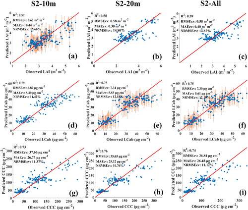
Figure 4. Scatterplots of the best MLRAs for each of the spectral configurations, i.e. S2-10m (a, d, g), S2-20m (b, e, h) and S2-All (c, f, i) in Harrismith. The best LAI (a–c) and LC_ab results (d–f) were by GPR for all MSI configurations, i.e. using S2-10m, S2-20m, and S2-All. (g), (h), and (i) shows the best CCC results obtained by GPR using S2-10m, RF using S2-20m, and XGBoost using S2-All, respectively.

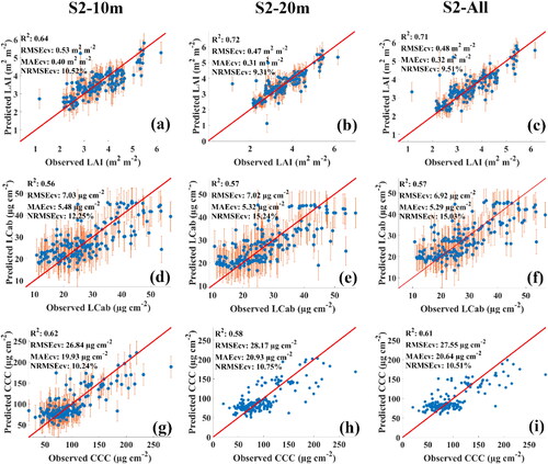
Figure 5. Maps generated by the best models with S2-10m and S2-20m data in Bothaville (a–f) and Harrismith (g–l). (a) and (d) show the best LAI (m² m⁻²) results using GPR (S2-10m) and RF (S2-20m), (b) and (e) show the best LC_ab (µg cm⁻²) results using XGBoost (S2-10m) and GPR (S2-20m), and (c) and (f) show the best CCC (µg cm⁻²) results using XGBoost for both S2-10m and S2-20m in Bothaville. (g) and (j) show the best LAI model using GPR for both S2-10m and S2-20m, (h) and (k) show best LC_ab model results using GPR with both S2-10m and S2-20m, and (j) and (l) show the best CCC results using GPR (S2-10m) and RF (S2-20m), respectively.

Figure 6. Biophysical and biochemical parameters maps generated by the best GPR models with S2-10m and S2-20m data in Bothaville (a–b) and Harrismith (e–g). (c), (d), (h)–(j) are the pixel-wise uncertainties coefficient of variation (CV, %).

Spatial distribution maps for optimal MSI spectral configurations and MLRA models

The spatial distribution maps of LAI, LC_ab and CCC from S2-10m and S2-20m and the best MLRA models (i.e. corresponding to the scatter plots above) at the two sites are given in Figure 5, while the best GPR models and their associated uncertainty layers (i.e. coefficient of variation, CV) are presented in Figure 6. Figure 5(a) shows the detailed within-field LAI spatial variations achieved by the S2-10m-GPR-LAI model. As shown in Figure 6(d), higher LAI values (i.e. >4 m² m⁻²) over circular irrigated fields had lower uncertainties, i.e. CV < 20%, while the surrounding regular (usually rainfed fields) had relatively higher uncertainties, i.e. 20%>CV < 40%. In contrast, the S2-20m-RF-LAI results, i.e. Figure 5(d), display relatively less within-field variability. In Harrismith, the S2-10m-GPR-LAI model, i.e. Figure 5(g), shows relatively low LAI values, while the S2-20m-GPR-LAI model, i.e. Figure 5(j), show relatively high values for most fields. The S2-20m-GPR-LAI model which achieved the best RMSE, i.e. Figure 6(j), shows uncertainties similar to Bothaville, where higher LAI values (i.e. >4 m² m⁻²) exhibited lower uncertainties, i.e. CV <20%, while LAI values of ∼3 to 4 m² m⁻² had a CV of between 20 and 40% (see Figure 6j). These uncertainties were mainly due to the presence of senescent (brown) leaves at the time of the field measurements, associated with the physiological maturity stage, while other fields were almost completely senescent. These fields may have had higher NDVI values than the threshold used to mask green vegetation, i.e. 0.2.

The spatial distribution of LC_ab between the two configurations was different, with S2-20m showing higher values over irrigated (circular) fields (Figure 5e), while S2-10m values over the same fields were relatively lower (Figure 5b). The rainfed (regular) fields also exhibited relatively lower LC_ab values. The Bothaville results using the S2-20m configuration were achieved with GPR, while the S2-10m results were obtained with XGBoost. Generally, the same patterns can be observed in Harrismith using both configurations and GPR. The uncertainty maps obtained with the best GPR models only, i.e. Figure 6(e) and 6(k), also show higher uncertainties (i.e. 20%>CV < 40%) where LC_ab values are relatively low (<20 µg cm⁻²), and better uncertainties (CV <20%) over irrigated fields with relatively high LC_ab values (> 40 µg cm⁻²).

The spatial distribution maps of CCC obtained with XGBoost for both S2-10m and S2-20m configurations, in Bothaville, show no obvious differences (Figure 5c and 5f). In Harrismith, some differences between the two configurations are evident particularly over rainfed fields with relatively low CCC values (Figure 4i and 4l), which can be two attributed to the fact that they were generated by two different algorithms and spectral configurations. The GPR uncertainties, which were applicable for Harrismith only (Figure 6l), show CV over 60% in some parts of the rainfed fields. While the spatial resolution was not of interest here, it may have played a role in the variations in spatial distributions of the retrieved biophysical and biochemical parameters. S2-10m provided finer details with greater within-field variability than S2-20m.

Discussion

The advent of Copernicus Sentinel-2 twin-satellites has provided prospects to improve crop biophysical and biochemical retrieval accuracy as well as the frequency and level of detail relevant for precision agriculture and crop monitoring needs. Its improved spectral configuration, i.e. with new RE-bands, centred at 705 nm, 740 nm, and 783 nm, has increased interest in their utility for crop biophysical and biochemical parameters retrieval using various methods. Of interest here, is the performance of the two Sentinel-2 spectral configurations, i.e. providing four standard multispectral bands in the VNIR region at 10 m spatial resolution (i.e. S2-10m) and six bands in the RE-NIR-SWIR regions at 20 m spatial resolution (i.e. S2-20m), in retrieving LAI, LC_ab and CCC using three robust MLRAs in two semi-arid agricultural sites, i.e. Bothaville and Harrismith. The two configurations were benchmarked against the full MSI spectral data (S2-All), consisting of 10 bands, covering VIS, RE, NIR, and SWIR spectral regions all resampled to a spatial resolution of 10 m.

Performance of MSI configurations for crop biophysical and biochemical parameters retrieval

The VNIR spectral region of the electromagnetic spectrum (i.e. 350 nm–649 nm), sampled by S2-10m spectral bands, contains the fundamental vegetation absorption regions that have allowed image-based vegetation characterisation for decades (Tucker 1979; Pinty and Verstraete 1992; Myneni and Williams 1994; Myneni et al. 2002; Brown et al. 2006; Zhu et al. 2013). Sentinel-2 B2:490 nm and B4:665 nm coincide with the widely known intense absorption by pigments such as xanthophyll, anthocyanin, chlorophyll, and carotenoid, while B8:560 nm exhibits a high scattering effect caused by the canopy structure, spongy mesophyll cells, and water content in leaves (Jensen 1983; Blackburn 1998). Therefore, it is not surprising that VNIR bands are one of the predominant predictors of biophysical and biochemical parameters in various retrieval approaches and environmental settings, despite the spectral resolution, range and number of bands of the input dataset (Delegido et al. 2011; Verrelst et al. 2016). For example, Delegido et al. (2011) found that a normalised difference index (NDI) constructed with CHRIS (Compact High-Resolution Imaging Spectroscopy) hyperspectral bands centred at 674 nm (i.e. near S2-B4:665 nm) and 712 nm (i.e. near S2-B5:705 nm) were not only the best predictors of LAI but were also portable to a simulated Sentinel-2 image, resulting in uncertainty (i.e. RMSE) of 0.6 m² m⁻². In the current study, the S2-10m configuration—characterised by broad bandwidth bands (i.e. B2:490 nm, B3:560 nm, B4:665 nm and B8:842 nm)—resulted in comparable LAI uncertainty (i.e. RMSE_cv) of between 0.62 m² m⁻² and 0.53 m² m⁻² in Bothaville and Harrismith, respectively. Consistently, Verrelst et al. (2016) found that the bands centred at 462 nm (blue) and 1327 nm (NIR) were among the four optimal bands (of the 125 HyMap spectral bands) for LAI retrieval at low uncertainties (i.e. RMSE_cv of 0.37 m² m⁻² and R² of 0.95). However, as shown, their results were significantly better than the ones obtained here because they used hyperspectral data with narrow bandwidths (i.e. 11 nm and 21 nm) and two of the four optimal bands (i.e. centred at 708 nm and 723 nm) are positioned in the red-edge region. Although the utility of hyperspectral data has been shown extensively demonstrated in the literature (Zhao et al. 2011; Yi et al. 2014; Yu et al. 2017; Wen et al. 2020), the lack of operational space-based sensors hinders its practical application.

Sentinel-2’s narrow bands, i.e. B5:705 nm, B6:740 nm, B7:783 nm, and B8A:865 nm at 20 m spatial resolution, are therefore a good compromise and essential for the detailed (field-level) characterisation of essential biophysical and biochemical parameters for agronomic applications. The contribution of the red-edge bands is shown in the results of the S2-20m configuration (in this study)—characterised by the three red-edge bands, one narrow NIR band and two SWIR spectral bands (i.e. B11:1610 nm and B12:2190 nm)—which were robust in consistently retrieving LAI with relatively low uncertainties (RMSE_cv) of 0.58 m² m⁻² and 0.47 m² m⁻² in Bothaville and Harrismith, respectively. The S2-20m LAI uncertainties were slightly better than those obtained with S2-10m at both sites. Therefore, the results show a combined effect of chlorophyll content, plant structure, and foliar moisture content—which control the reflectance in the RE, NIR, and SWIR regions—were more influential in the retrieval of LAI. The RE region is sensitive to changes in chlorophyll, thus averting the saturation effect caused by this pigment in the VIS region. For example, VNIR data often saturates and fails to accurately characterise medium (i.e. ∼3 m² m⁻²) to high (i.e. >5 m² m⁻²) LAI values, while the inclusion of RE bands improves the dynamic range of these biophysical and biochemical parameters (Peng and Gitelson 2011). A benchmark of S2-20m’s performance to S2-All showed proportionate performance, which implies that broadband VNIR can be discarded in the retrieval of LAI.

These results are comparable to Campos-Taberner et al. (2016) who found similar uncertainties over Mediterranean Rice in Spain, i.e. RMSE: 0.39 m² m⁻² and 0.51 m² m⁻², and Italy, i.e. 0.38 m² m⁻² and 0.47 m² m⁻², using Landsat and SPOT-5 data, respectively. Therefore, this also shows that the Sentinel-2 SWIR bands, which are similar to those of Landsat and SPOT data, were also essential in achieving low uncertainties with S2-20m in this study. The contribution of SWIR bands (B11:1610 nm and B12:2190 nm) to LAI accuracy is mostly because they are affected by foliar moisture content, which plays an important role in the critical developmental (vegetative and productive) stages of crops, hence controlling the abundance of biophysical and biochemical traits such as canopy structure and chlorophyll content (Curran 2001; Verrelst et al. 2015). Essentially, the availability or deficiency of water determines the productivity and yield of an agricultural system. When crops reach physiological maturity (as in our case), moisture content declines steadily, thus causing a decline in leaf chlorophyll content and loss of greenness, while LAI may remain moderately high. In a related study utilising the entire Sentinel-2 spectral data (resampled to 20 m) in Bothaville (Kganyago et al. 2021), B11:1610 nm and B12:2190 nm were in the top five most influential bands in the LAI model, helping achieve a comparable (to the current study) RMSE of 0.5 m² m⁻² using RF algorithm. Consistently, Verrelst et al. (2015) also found that Sentinel-2 SWIR bands were among the relevant spectral bands for retrieving LAI with the Variational Heteroscedastic GPR (VH-GPR) model with RMSE_cv of 0.44 m² m⁻² and R² of 0.90. In the current study, the benchmarking results using S2-All further ascertained the relative contribution of RE, NIR and SWIR bands, leading to the assumption that the location, bandwidth, and spectral regions where the bands were sampled (i.e. the spectral configuration) was more important than spatial resolution for LAI retrieval. This is consistent with Kganyago et al. (2020) who found no significant difference between Sentinel-2 resolutions in retrievals of LAI using a pre-trained hybrid Radiative Transfer Model (RTM) and Artificial Neural Networks (ANN) model.

The results also showed that LC_ab could be retrieved with relatively low uncertainties of 6.89 µg cm⁻² and 7.02 µg cm⁻² with S2-10m at the two sites, respectively. This finding is consistent with Clevers et al. (2017) who found that vegetation indices constructed from VNIR (i.e. S2-10m) spectral bands such as the Weighted Difference Vegetation Index (WDVI), Green Chlorophyll Index (CI_green), and Chlorophyll Vegetation Index (CVI) were more robust than those computed from red-edge (i.e. S2-20m) spectral bands such as Red-edge Chlorophyll Index (CI_red-edge), the ratio of Transformed Chlorophyll in Reflectance Index and Optimised Soil-adjusted Vegetation Index (TCARI/OSAVI) in retrieving LAI, LC_ab, CCC for Potato crops. Moreover, using GPR-BAT (GPR-based band analysis tool) on the field hyperspectral data, Verrelst et al. (2016) found that LC_ab could be accurately estimated with bands centred at 482 nm (blue), 500 nm and 564 nm (i.e. green peak), 710 nm and 714 nm (red edge) and a region between 878–980 nm (NIR) with NRMSE_cv < 10%. The red-edge spectral bands in Verrelst et al. (2016), i.e. 710 nm and 714 nm, are closer to Sentinel-2 B5:705 nm, which was found to be one of the most influential bands alongside B3:560 nm, B4:665 nm, B11:1610 nm, B12: 2190 nm, in the MLRA retrieval of LC_ab, achieving uncertainties of 7.57 µg cm⁻² (Kganyago et al. 2021). In the current study, the contribution of these spectral bands (i.e. S2-20m) in the retrieval of LC_ab was evident, achieving equivalently lower uncertainties as S2-10m, i.e. 7.02 µg cm⁻², in Harrismith.

The benchmark results, using S2-All, did not result in any significant variations in estimates in relation to S2-10m, demonstrating the usefulness of VNIR bands. The results imply that spectrally limited datasets such as those from SPOT 6/7, PlanetScope Doves and low-cost UAV platforms can be used for crop nitrogen management since studies established that LC_ab is highly correlated with N-content (Jia et al. 2013; Vincini et al. 2016). This also means that small crop damage due to biotic (e.g. pests and diseases) and abiotic (e.g. water, temperature, and nutrients) stress factors can be detected early (i.e. before it becomes widespread) due to the high detail provided by these systems, thus potentially providing better prospects of early crop stress mitigation and high yields. However, as shown by the results (Tables 2 and 3), S2-20m and S2-All also provided equally good results; therefore, where RE, NIR and SWIR spectral bands are available, they should be used to reduce systematic errors and improve the range of retrieved values in line with previous studies (Verrelst et al. 2012; Vincini et al. 2016). For CCC, the best configurations were different at the two sites, where S2-20m was better in Bothaville (RMSE_cv: 35.65 µg cm⁻²) and S2-10m was better in Harrismith (i.e. RMSE_cv: 26.84 µg cm⁻²). The inconsistencies may be due to slightly different conditions at the two sites, where CCC (a product of LAI and LC_ab) in Harrismith was mainly influenced by chlorophyll content than the one in Bothaville, where plant structure and water content played a major role. This is reasonable since fieldwork dates between Harrismith and Bothaville were slightly different, i.e. March and April, respectively. Since the crop calendar is the same for both sites, Bothaville had relatively lower LC_ab, and its influence on CCC was relatively minimal when compared to LAI. Using S2-All did not improve the CCC results by S2-20m (in Bothaville) and S2-10m (in Harrismith), implying that either 10 m or 20 m MSI spectral bands can be applied without the need to use all resampled bands. The results of S2-20m and S2-10m achieved here, are slightly better than those found in a related previous study (Kganyago et al. 2021), where CCC retrieval with resampled Sentinel-2 bands to 20 m achieved RMSE of 39.49 µg cm⁻².

The utility of S2-10m and S2-20m for various parameters is essential for the rapid assessment of the crop biophysical and biochemical parameters, without delays caused by additional pre-processing steps such as downsampling the S2-10m or upsampling the S2-20m spectral bands, and applying super-resolving techniques (Zhang et al. 2019), before retrieval; thus, the results from this study have operational significance. In our study, upsampling to 10 m caused 7 min and 17.787 s delay for a single Sentinel-2 tile consisting of width and height of 10,980 pixels on an Intel® Core™ i7-8700 CPU and 64 GB RAM. Moreover, S2-10m results obtained here are significant for informing biophysical and biochemical parameter retrieval using other sensors such as Planet Doves or low-cost UAVs, which only have VNIR bands and higher or flexible temporal resolution. However, all configurations had a rather relatively lower R² in Harrismith, explaining the variability of between 54% to 72%, 53% to 57%, and 57% to 62%, for LAI, LC_ab, and CCC, respectively. In contrast, only LAI in Bothaville achieved a similar accuracy (R²) of 52% to 58%, while the variability of LC_ab and CCC was relatively well-explained by the two configurations, with R² of 75% to 79% and 69% to 76%, respectively. The lower R² may be linked to the diverse structural forms within the same area emanating from different crop types and planting times. Nonetheless, all R² were above 50%, while NRMSE_cv was below 20%, thus within limits recommended by the Global Climate Observing System (GCOS) (GCOS 2011).

Effect of various MSI configurations on the performance of MLRAs

The above results were achieved with three state-of-art MLRAs, i.e. RF, XGBoost and GPR. As shown by the results (Figures 3 and 4), the MLRAs considered here were generally sensitive to various Sentinel-2 MSI configurations, i.e. S2-10m (i.e. four bands), S2-20m (i.e. six bands), and S2-All (10 bands), out-competing each other for each configuration and biophysical and biochemical parameter. Although RF and XGBoost had similar performances—attributed to their similar tree-based origin—XGBoost was superior in most cases in retrieving crop biophysical and biochemical parameters in both Bothaville and Harrismith and using all Sentinel-2 configurations. While RF uses bagging, randomly selected variables at each split, and many trees for predictions. In contrast, XGBoost introduces gradient boosted decision trees and computational efficiency for thousands of trees, thus having better flexibility, efficiency avoiding overfitting and is sparsity-aware (Chen and Guestrin 2016). The slightly better performance of XGBoost found here, is consistent with previous studies (Bahrami et al. 2021; Zhang et al. 2021). Generally, tree-based algorithms are attractive because they are simple to understand, transparent and explainable, i.e. tree structure, splitting points and variables for each decision, and influential variables can be interrogated to understand how they operate in different scenarios. However, the results showed that GPR was more robust in most cases (see Figures 3 and 4), resulting in better estimates even when only four bands (S2-10m) were used. Despite its ‘black-box’ nature, GPR strength lies in providing the per-pixel uncertainty estimates, which can be used to decide an uncertainty threshold in operational settings (Amin et al. 2021). In previous studies, GPR uncertainty measures, i.e. standard deviation and coefficient of variation, had been used to also exclude uncertainty from fallow and non-crop areas (Verrelst et al. 2013). Overall, MLRAs evaluated here, showed sensitivity to different datasets (i.e. S2-10m, S2-20m, and S2-All) and experimental sites (Bothaville and Harrismith). This implies that it is essential to evaluate various MLRAs, before choosing the optimal one for specific spectral configuration, application and crop conditions. Consequently, software tools such as ARTMO Machine Learning Regression Algorithm (MLRA) toolbox (Rivera et al. 2014; Verrelst et al. 2012)—which provide an intuitive platform for rapidly and simultaneously computing multiple MLRAs—are essential to achieving improved crop biophysical and biochemical parameters and their rapid dissemination to users. Recent studies show the integration of ARTMO generated coefficients with satellite data cloud APIs such as Google Earth Engine (GEE) to enable rapid upscaling of crop biophysical and biochemical parameters such as LAI (Pipia et al. 2021; Estévez et al. 2022). Therefore, it would be interesting to extend the results obtained here, i.e. with different Sentinel-2 configurations, to other areas. In such a case, hybrid models (e.g. RTM-MLRA) should be considered, since experimental data are limited to the measured crop types and conditions and affected by prevailing climatic and environmental conditions.

Although comparable with previous studies, our results for the S2-10m configuration were likely impacted by the Sentinel-2 B2:490 nm, which is known to exhibit residual atmospheric effects that may have introduced uncertainties in the crop biophysical and biochemical retrievals using MLRAs. Another source of uncertainty may be the high correlation between the B2:490 nm and B4:665 nm, which may have introduced collinearity due to their similar vegetation spectral response in these bands (i.e. pronounced absorption), as well as saturation due to chlorophyll absorption. Nonetheless, the usefulness of the blue band has been demonstrated in the Enhanced Vegetation Index (EVI) formulation to account for atmospheric effects and avoid the saturation effect of NDVI at high (i.e. 6 m² m⁻²) and low (i.e. <2 m² m⁻²) LAI values. Moreover, it featured prominently in the biophysical and biochemical parameters retrieval models in recent studies (Verrelst et al. 2016; Kganyago et al. 2021). Therefore, the sensitivity of the MLRA retrieval models to B2:490 nm effects must be evaluated in greater detail, in tandem with the efforts to quantify the magnitude of these residual errors from various atmospheric correction techniques (i.e. including Sen2Cor used here). Lastly, although there was a fair balance between Maize (i.e. 63.94% and 62.01%) and Beans (i.e. 32.56% and 49.72%) at the two sites, respectively, Peanuts (i.e. present in Bothaville only) were the least represented, i.e. 3.49%. Beside the machine learning algorithms being renowned for robustness to imbalanced training samples, we cannot eliminate the possibility that this may have had an effect on performance of the MLRA models. Crop-specific models will be considered in our future works.

Conclusions

This study assessed the utility of the two Sentinel-2 spectral configurations that provide four standard multispectral bands in the VNIR region at 10 m spatial resolution (i.e. S2-10m) and six bands in the RE-NIR-SWIR regions at 20 m spatial resolution (i.e. S2-20m), in retrieving crop biophysical and biochemical parameters, i.e. LAI, LC_ab and CCC, using three robust MLRAs in two semi-arid agricultural sites, i.e. Bothaville and Harrismith. The results were compared to those obtained with all spectral bands (S2-All). In summary, the results showed that the S2-20m configuration—with four narrow bands and two SWIR bands—was more robust, when compared to S2-10, in retrieving LAI with low uncertainties (i.e. RMSE_cv: 0.58 m² m⁻² and 0.47 m² m⁻²) in the two sites, respectively. In contrast, the S2-10m configuration was relatively better in retrieving LC_ab in both sites (RMSE_cv: 6.89 µg cm⁻² and 7.02 µg cm⁻²). However, S2-20m was equally robust in Harrismith, in achieving equivalent uncertainties as S2-10m, i.e. RMSE_cv: 7.02 µg cm⁻². This shows the relevance of red-edge bands in biophysical and biochemical parameters retrieval as shown by previous studies (Mutanga and Skidmore 2007; Verrelst et al. 2012). However, the results in the current study showed that VNIR bands could perform better than red-edge bands when it comes to retrieving LC_ab. Regarding CCC, the performance of the two configurations was not consistent in the two sites, where S2-20m performed better in Bothaville with RMSE_cv: 35.65 µg cm⁻², but not in Harrismith, where S2-10m yielded relatively lower uncertainties with RMSE_cv of 26.84 µg cm⁻². The obtained results are slightly better than those of a related study utilising resampled Sentinel-2 bands at 20 m (Kganyago et al. 2021). Moreover, all the configurations yielded accuracies that were slightly better or equivalent to the benchmark dataset consisting of resampled bands to 10 m, i.e. S2-All. The better performance of S2-10m in the retrieval of LC_ab and CCC found here, may inform biophysical and biochemical parameters retrieval from similar high-resolution data with VNIR data from SPOT 6/7, PlanetScope Doves and low-cost UAV platforms, essential for crop nitrogen management at field-level. However, it should be noted that the S2-10m results obtained here, may have been affected by the inclusion of the blue band (i.e. B2), which contains residual atmospheric effects, correlated to the red band (i.e. B4) due to similar vegetation spectral response, and saturation effects in the red band due to the high chlorophyll content. Future studies should assess the sensitivity of the MLRA retrieval models to the blue band effects in greater detail. The results imply that both Sentinel-2 configurations can be used independently since there was no marked difference between all configurations (i.e. S2-10m and S2-20m) and the resampled bands (S2-All). Further analyses in other areas are required to ascertain the findings in the current study since the biophysical and biochemical retrieval models developed here used experimental data, which are limited to the measured crop types and conditions and affected by prevailing climatic and environmental conditions. While GPR was robust in most cases, RF and XGBoost were also robust in others, thus indicating that all MLRAs evaluated here are sensitive to various spectral configurations and study areas. Therefore, it becomes essential to evaluate various MLRAs, before choosing the optimal one for specific biophysical and biochemical parameters. Overall, the results inform future retrieval of essential crop biophysical and biochemical parameters from the two Sentinel-2 configurations to support time-sensitive precision agronomic applications.

Authors’ contributions

Conceptualization, M.K. and C.A.; methodology, M.K.; formal analysis, M.K.; writing—original draft preparation, M.K. and M.S.; writing—review and editing, M.K., C.A. P.M., M.S. T.A., and G.L.; visualization, M.K.; super-vision, C.A. P.M. T.A., and G.L. All authors have read and agreed to the published version of the manuscript.

Acknowledgments

The authors appreciate the ESA Network of Resources (NoR) sponsorship for funding the subscription to Sentinel Hub Cloud API for Satellite Imagery used in this study, the University of the Witwatersrand for the Postgraduate Merit Award (PMA) and field data from the EU-H2020 AfriCultuReS project, which received funding from the European Union’s Horizon 2020 Research and Innovation Framework Programme under grant agreement No. 774652. The support provided by the South African National Space Agency (SANSA) is highly appreciated, particularly the participation of Nosiseko Mashiyi, Morwapula Mashalane, and Lesiba Tsoeleng, as well as Andiswa Silinga and Tiisetso Kekana from Gemini GIS and Environmental Services during fieldwork. We also thank the farmers in Bothaville and Harrismith for welcoming us to their fields for data collection. Last but not least, we thank anonymous reviewers and editor(s) for taking the time to provide constructive feedback that shaped this manuscript. We appreciate free access to ARTMO software and associated toolboxes through a Research/Academic license.

Disclosure statement

The authors declare that they have no conflict of interest.

Additional information

Funding

This research was supported by the AfriCultuReS project, which received funding from the European Union’s Horizon 2020 Research and Innovation Framework Programme under grant agreement No. 774652. Mahlatse Kganyago received European Space Agency (ESA) Network of Resources (NoR) sponsorship for Sentinel Hub (by Synergise) subscription. Mahlatse Kganyago received a Postgraduate Merit Award (PMA) and a Bursary from the University of the Witwatersrand.

References

- Amin E, Verrelst J, Rivera-Caicedo JP, Pipia L, Ruiz-Verdú A, Moreno J. 2021. Prototyping Sentinel-2 green LAI and brown LAI products for cropland monitoring. Remote Sens Environ. 255:112168.
- Ayumi V. 2017. Pose-based human action recognition with extreme gradient boosting. Proceedings - 14th IEEE Student Conference on Research and Development: Advancing Technology for Humanity, SCOReD 2016. IEEE.
- Bahrami H, Homayouni S, Safari A, Mirzaei S, Mahdianpari M, Reisi-Gahrouei O. 2021. Deep learning-based estimation of crop biophysical parameters using multi-source and multi-temporal remote sensing observations. Agronomy. 11(7):1363.
- Beltran JC, Valdez P, Naval P. 2019. Predicting protein-protein interactions based on biological information using extreme gradient boosting. 2019 IEEE Conference on Computational Intelligence in Bioinformatics and Computational Biology (CIBCB).
- Blackburn GA. 1998. Quantifying chlorophylls and caroteniods at leaf and canopy scales: an evaluation of some hyperspectral approaches. Remote Sens Environ. 66(3):273–285.
- Breiman L. 2001. Random forests. Mach Learn. 45(1):5–32.
- Breiman L, Friedman JH, Olshen RA, Stone CJ. 1984. Classification and regression trees. New York: Wadsworth International Group.
- Brown ME, Pinzón JE, Didan K, Morisette JT, Tucker CJ. 2006. Evaluation of the consistency of long-term NDVI time series derived from AVHRR, SPOT-vegetation, SeaWiFS, MODIS, and Landsat ETM + sensors. IEEE Trans Geosci Remote Sens. 44(7):1787–1793.
- Camacho F, Fuster B, Li W, Weiss M, Ganguly S, Lacaze R, Baret F. 2021. Crop specific algorithms trained over ground measurements provide the best performance for GAI and fAPAR estimates from Landsat-8 observations. Remote Sens Environ. 260:112453.
- Campos-Taberner M, García-Haro FJ, Camps-Valls G, Grau-Muedra G, Nutini F, Crema A, Boschetti M. 2016. Multitemporal and multiresolution leaf area index retrieval for operational local rice crop monitoring. Remote Sens Environ. 187:102–118.
- Camps-Vails G, Gómez-Chova L, Muñoz-Mari J, Vila-Francés J, Amoros J, del Valle-Tascon S, Calpe-Maravilla J. 2009. Biophysical parameter estimation with adaptive Gaussian processes. 2009 IEEE International Geoscience and Remote Sensing Symposium.
- Camps-Valls G, Gómez-Chova L, Muñoz-Marí J, Lázaro-Gredilla M, Verrelst J. 2013. simpleR: a simple educational Matlab toolbox for statistical regression. V2. https://www.uv.es/gcamps/software.html (accessed 10 December 2018).
- Camps-Valls G, Verrelst J, Munoz-Mari J, Laparra V, Mateo-Jimenez F, Gomez-Dans J. 2016. A survey on Gaussian processes for earth-observation data analysis: a comprehensive investigation. IEEE Geosci Remote Sens Mag. 4:58–78.
- Chemura A, Mutanga O, Odindi J. 2017. Empirical modeling of leaf chlorophyll content in coffee (Coffea arabica) plantations with Sentinel-2 MSI data: effects of spectral settings, spatial resolution, and crop canopy cover. IEEE J Sel Top Appl Earth Observ Remote Sens. 10(12):5541–5550.
- Chen T, Guestrin C. 2016. Xgboost: a scalable tree boosting system. Proceedings of the 22nd ACM SIGKDD International Conference on Knowledge Discovery and Data Mining.
- Chrysafis I, Korakis G, Kyriazopoulos AP, Mallinis G. 2020. Retrieval of leaf area index using Sentinel-2 imagery in a mixed Mediterranean forest area. IJGI. 9(11):622.
- Clevers J, Kooistra L, Van Den Brande M. 2017. Using Sentinel-2 data for retrieving LAI and leaf and canopy chlorophyll content of a potato crop. Remote Sens. 9(5):405.
- Collins W. 1978. Remote sensing of crop type and maturity. Photogramm Eng Remote Sens. 44(1):43–55.
- Croft H, Arabian J, Chen JM, Shang J, Liu J. 2020. Mapping within-field leaf chlorophyll content in agricultural crops for nitrogen management using Landsat-8 imagery. Precision Agric. 21(4):856–880.
- CropEstimatesConsortium. 2017. Field Crop Boundary data layer (Free State province). Department of Agriculture, Forestry and Fisheries, Pretoria, South Africa.
- Curran PJ. 2001. Imaging spectrometry for ecological applications. Int J Appl Earth Obs Geoinf. 3(4):305–312.
- da Silva Jr CA, Teodoro LPR, Teodoro PE, Baio FHR, Pantaleão AdA, Capristo-Silva GF, Facco CU, Oliveira-Júnior JFd, Shiratsuchi LS, Skripachev V, et al. 2020. Simulating multispectral MSI bandsets (Sentinel-2) from hyperspectral observations via spectroradiometer for identifying soybean cultivars. Remote Sens Appl: Soc Environ. 19:100328.
- Delegido J, Verrelst J, Alonso L, Moreno J. 2011. Evaluation of sentinel-2 red-edge bands for empirical estimation of green LAI and chlorophyll content. Sensors (Basel). 11(7):7063–7081.
- Delegido J, Verrelst J, Meza CM, Rivera JP, Alonso L, Moreno J. 2013. A red-edge spectral index for remote sensing estimation of green LAI over agroecosystems. Eur J Agron. 46:42–52.
- Delegido J, Verrelst J, Rivera JP, Ruiz-Verdú A, José Moreno J. 2015. Brown and green LAI mapping through spectral indices. Int J Appl Earth Obs Geoinf. 35:350–358.
- Delloye C, Weiss M, Defourny P. 2018. Retrieval of the canopy chlorophyll content from Sentinel-2 spectral bands to estimate nitrogen uptake in intensive winter wheat cropping systems. Remote Sens Environ. 216:245–261.
- Drusch M, Del Bello U, Carlier S, Colin O, Fernandez V, Gascon F, Hoersch B, Isola C, Laberinti P, Martimort P, et al. 2012. Sentinel-2: ESA's optical high-resolution mission for GMES operational services. Remote Sens Environ. 120:25–36.
- Du P, Samat A, Waske B, Liu S, Li Z. 2015. Random forest and rotation forest for fully polarized SAR image classification using polarimetric and spatial features. ISP RS J Photogramm Remote Sens. 105:38–53.
- Estévez J, Salinero-Delgado M, Berger K, Pipia L, Rivera-Caicedo JP, Wocher M, Reyes-Muñoz P, Tagliabue G, Boschetti M, Verrelst J. 2022. Gaussian processes retrieval of crop traits in Google Earth Engine based on Sentinel-2 top-of-atmosphere data. Remote Sens Environ. 273:112958.
- Estévez J, Vicent J, Rivera-Caicedo JP, Morcillo-Pallarés P, Vuolo F, Sabater N, Camps-Valls G, Moreno J, Verrelst J. 2020. Gaussian processes retrieval of LAI from Sentinel-2 top-of-atmosphere radiance data. ISPRS J Photogramm Remote Sens. 167:289–304.
- Fawagreh K, Gaber MM, Elyan E. 2014. Random forests: from early developments to recent advancements. Syst Sci Control Eng. 2(1):602–609.
- Friedman JH. 2001. Greedy function approximation: a gradient boosting machine. Ann Stat. 29(5):1189–1232.
- Gao F, Anderson MC, Zhang X, Yang Z, Alfieri JG, Kustas WP, Mueller R, Johnson DM, Prueger JH. 2017. Toward mapping crop progress at field scales through fusion of Landsat and MODIS imagery. Remote Sens Environ. 188:9–25.
- GCOS. 2011. Systematic observation requirements for satellite-based products for climate. In Supplemental details to the satellite-based component of the Implementation Plan for the Global Observing System for Climate in Support of the UNFCCC: 2011 update, 2011 update ed., Vol. GCOS - No. 154, p. 138. Geneva, Switzerland: World Meteorological Organization (WMO).
- Gislason PO, Benediktsson JA, Sveinsson JR. 2006. Random Forests for land cover classification. Pattern Recog Lett. 27(4):294–300.
- Gitelson AA, Peng Y, Masek JG, Rundquist DC, Verma S, Suyker A, Baker JM, Hatfield JL, Meyers T. 2012. Remote estimation of crop gross primary production with Landsat data. Remote Sens Environ. 121:404–414.
- Godfray HCJ, Garnett T. 2014. Food security and sustainable intensification. Philos Trans R Soc Lond B Biol Sci. 369(1639):20120273.
- Guan H, Li J, Chapman M, Deng F, Ji Z, Yang X. 2013. Integration of orthoimagery and lidar data for object-based urban thematic mapping using random forests. Int J Remote Sens. 34(14):5166–5186.
- Gupta A, Gusain K, Popli B. 2016. Verifying the value and veracity of extreme gradient boosted decision trees on a variety of datasets. 2016 11th International Conference on Industrial and Information Systems (ICIIS), pp. 457–462.
- Jacquemoud S, Verhoef W, Baret F, Bacour C, Zarco-Tejada PJ, Asner GP, François C, Ustin SL. 2009. PROSPECT + SAIL models: a review of use for vegetation characterization. Remote Sens Environ. 113: S56–S66.
- Jensen JR. 1983. Biophysical remote sensing. Ann Assoc Am Geogr. 73(1):111–132.
- Jia F, Liu G, Liu D, Zhang Y, Fan W, Xing X. 2013. Comparison of different methods for estimating nitrogen concentration in flue-cured tobacco leaves based on hyperspectral reflectance. Field Crops Res. 150:108–114.
- Kganyago M. 2021. Using sentinel-2 observations to assess the consequences of the COVID-19 lockdown on winter cropping in Bothaville and Harrismith, South Africa. Remote Sens Lett. 12(9):827–837.
- Kganyago M, Mhangara P, Adjorlolo C. 2021. Estimating crop biophysical parameters using machine learning algorithms and Sentinel-2 imagery. Remote Sens. 13(21):4314–4321.
- Kganyago M, Mhangara P, Alexandridis T, Laneve G, Ovakoglou G, Mashiyi N. 2020. Validation of sentinel-2 leaf area index (LAI) product derived from SNAP toolbox and its comparison with global LAI products in an African semi-arid agricultural landscape. Remote Sens Lett. 11(10):883–892.
- Kobayashi N, Tani H, Wang X, Sonobe R. 2020. Crop classification using spectral indices derived from Sentinel-2A imagery. J Inf Telecommun. 4(1):67–90.
- Lanaras C, Bioucas-Dias J, Baltsavias E, Schindler K. 2017. Super-resolution of multispectral multiresolution images from a single sensor. Proceedings of the IEEE Conference on Computer Vision and Pattern Recognition Workshops.
- Lanaras C, Bioucas-Dias J, Galliani S, Baltsavias E, Schindler K. 2018. Super-resolution of Sentinel-2 images: learning a globally applicable deep neural network. ISPRS J Photogramm Remote Sens. 146:305–319.
- Lawley V, Lewis M, Clarke K, Ostendorf B. 2016. Site-based and remote sensing methods for monitoring indicators of vegetation condition: an Australian review. Ecol Indic. 60:1273–1283.
- Loggenberg K, Strever A, Greyling B, Poona N. 2018. Modelling water stress in a Shiraz vineyard using hyperspectral imaging and machine learning. Remote Sens. 10(2):1–14.
- Louis J, Debaecker V, Pflug B, Main-Knorn M, Bieniarz J, Mueller-Wilm U, … Gascon F. 2016. Sentinel-2 Sen2Cor: l 2A processor for users. Proceedings Living Planet Symposium 2016.
- Ma Y, Liu S, Song L, Xu Z, Liu Y, Xu T, Zhu Z. 2018. Estimation of daily evapotranspiration and irrigation water efficiency at a Landsat-like scale for an arid irrigation area using multi-source remote sensing data. Remote Sens Environ. 216:715–734.
- Mango N, Siziba S, Makate C. 2017. The impact of adoption of conservation agriculture on smallholder farmers’ food security in semi-arid zones of southern Africa. Agric Food Secur. 6(1):1–8.
- Mansaray LR, Kanu AS, Yang L, Huang J. 2020. Dynamic modelling of rice leaf area index with quad-source optical imagery and machine learning regression models. Geocarto Int. 37(3):828–840.
- Maxwell E. 1976. Sensor design for monitoring vegetation canopies. Photogramm Eng Remote Sens. 42(11):1399–1410.
- Mueller-Wilm U. 2016. Sentinel-2 MSI—Level-2A prototype processor installation and user manual, 2016. Last accessed, 5.
- Mulla DJ. 2013. Twenty five years of remote sensing in precision agriculture: key advances and remaining knowledge gaps. Biosyst Eng. 114(4):358–371.
- Mutanga O, Skidmore AK. 2007. Red edge shift and biochemical content in grass canopies. ISPRS J Photogramm Remote Sens. 62(1):34–42.
- Myneni R, Williams D. 1994. On the relationship between FAPAR and NDVI. Remote Sens Environ. 49(3):200–211.
- Myneni RB, Hoffman S, Knyazikhin Y, Privette JL, Glassy J, Tian Y, Wang Y, Song X, Zhang Y, Smith GR, et al. 2002. Global products of vegetation leaf area and fraction absorbed PAR from year one of MODIS data. Remote Sens Environ. 83(1–2):214–231.
- Ndlovu HS, Odindi J, Sibanda M, Mutanga O, Clulow A, Chimonyo VGP, Mabhaudhi T. 2021. A comparative estimation of maize leaf water content using machine learning techniques and unmanned aerial vehicle (UAV)-based proximal and remotely sensed data. Remote Sensing. 13(20):4091. https://www.mdpi.com/2072-4292/13/20/4091.
- Pal M. 2005. Random forest classifier for remote sensing classification. Int J Remote Sens. 26(1):217–222.
- Parry C, Blonquist JM, Jr, Bugbee B. 2014. In situ measurement of leaf chlorophyll concentration: analysis of the optical/absolute relationship. Plant Cell Environ. 37(11):2508–2520.
- Pathy A, Meher S, Balasubramanian P. 2020. Predicting algal biochar yield using eXtreme Gradient Boosting (XGB) algorithm of machine learning methods. Algal Res. 50:102006.
- Peng Y, Gitelson AA. 2011. Application of chlorophyll-related vegetation indices for remote estimation of maize productivity. Agric For Meteorol. 151(9):1267–1276.
- Pinty B, Verstraete M. 1992. GEMI: a non-linear index to monitor global vegetation from satellites. Vegetatio. 101(1):15–20.
- Pipia L, Amin E, Belda S, Salinero-Delgado M, Verrelst J. 2021. Green lai mapping and cloud gap-filling using Gaussian process regression in google earth engine. Remote Sens (Basel). 13(3):403.
- Rasmussen CE. 2003. Gaussian processes in machine learning. In: Bousquet O, von Luxburg U, Rätsch G, editors. Advanced Lectures on on machine learning. Lecture Notes in Computer Science, Vol. 3176. Berlin, Heidelberg: Springer; p. 63–71.
- Richter K, Hank TB, Mauser W, Atzberger C. 2012. Derivation of biophysical variables from Earth observation data: validation and statistical measures. J Appl Remote Sens. 6(1):063557.
- Rivera-Caicedo JP, Verrelst J, Muñoz-Marí J, Camps-Valls G, Moreno J. 2017. Hyperspectral dimensionality reduction for biophysical variable statistical retrieval. ISPRS J Photogramm Remote Sens. 132:88–101.
- Rivera CJP, Verrelst J, Muñoz-Marí J, Moreno J, Camps-Valls G. 2014. Toward a semiautomatic machine learning retrieval of biophysical parameters. IEEE J Sel Top Appl Earth Obs Remote Sens. 7(4):1249–1259.
- Rodriguez-Galiano VF, Ghimire B, Rogan J, Chica-Olmo M, Rigol-Sanchez JP. 2012. An assessment of the effectiveness of a random forest classifier for land-cover classification. ISPRS J Photogramm Remote Sens. 67:93–104.
- Segarra J, Buchaillot ML, Araus JL, Kefauver SC. 2020. Remote sensing for precision agriculture: sentinel-2 improved features and applications. Agronomy. 10(5):641.
- Shah SH, Angel Y, Houborg R, Ali S, McCabe MF. 2019. A random forest machine learning approach for the retrieval of leaf chlorophyll content in wheat. Remote Sens. 11(8):920.
- Snee RD. 1977. Validation of regression models: methods and examples. Technometrics. 19(4):415–428.
- Tucker CJ. 1979. Red and photographic infrared linear combinations for monitoring vegetation. Remote Sens Environ. 8(2):127–150.
- Verrelst J, Alonso L, Camps-Valls G, Delegido J, Moreno J. 2012a. Retrieval of vegetation biophysical parameters using Gaussian process techniques. IEEE Trans Geosci Remote Sens. 50(5):1832–1843.
- Verrelst J, Muñoz J, Alonso L, Delegido J, Rivera JP, Camps-Valls G, Moreno J. 2012b. Machine learning regression algorithms for biophysical parameter retrieval: opportunities for Sentinel-2 and-3. Remote Sens Environ. 118:127–139.
- Verrelst J, Rivera JP, Gitelson A, Delegido J, Moreno J, Camps-Valls G. 2016. Spectral band selection for vegetation properties retrieval using Gaussian processes regression. Int J Appl Earth Obs Geoinf. 52:554–567.
- Verrelst J, Rivera JP, Moreno J, Camps-Valls G. 2013. Gaussian processes uncertainty estimates in experimental Sentinel-2 LAI and leaf chlorophyll content retrieval. ISPRS J Photogramm Remote Sens. 86:157–167.
- Verrelst J, Rivera JP, Veroustraete F, Muñoz-Marí J, Clevers JG, Camps-Valls G, Moreno J. 2015. Experimental Sentinel-2 LAI estimation using parametric, non-parametric and physical retrieval methods – A comparison. ISPRS J Photogramm Remote Sens. 108:260–272.
- Vincini M, Calegari F, Casa R. 2016. Sensitivity of leaf chlorophyll empirical estimators obtained at Sentinel-2 spectral resolution for different canopy structures. Precision Agric. 17(3):313–331.
- Walker RJ. 2016. Population growth and its implications for global security. Am J Econ Sociol. 75(4):980–1004.
- Wang L, Chang Q, Yang J, Zhang X, Li F. 2018. Estimation of paddy rice leaf area index using machine learning methods based on hyperspectral data from multi-year experiments. PLoS One. 13(12):e0207624.
- Wen P, Shi Z, Li A, Ning F, Zhang Y, Wang R, Li J. 2020. Estimation of the vertically integrated leaf nitrogen content in maize using canopy hyperspectral red edge parameters. Precis Agric. 22:984–1005.
- Williams CK, Rasmussen CE. 2006. Gaussian processes for machine learning. Vol. 2. Cambridge, MA: MIT Press.
- Xie Q, Dash J, Huete A, Jiang A, Yin G, Ding Y, Peng D, Hall CC, Brown L, Shi Y, et al. 2019. Retrieval of crop biophysical parameters from Sentinel-2 remote sensing imagery. Int J Appl Earth Obs Geoinf. 80:187–195.
- Yi Q, Wang F, Bao A, Jiapaer G. 2014. Leaf and canopy water content estimation in cotton using hyperspectral indices and radiative transfer models. Int J Appl Earth Obs Geoinf. 33(1):67–75.
- Yu FH, Xu TY, Du W, Ma H, Zhang GS, Chen CL. 2017. Radiative transfer models (RTMs) for field phenotyping inversion of rice based on UAV hyperspectral remote sensing. Int J Agric Biol Eng. 10(4):150–157.
- Zhang M, Su W, Fu Y, Zhu D, Xue J-H, Huang J, Wang W, Wu J, Yao C. 2019. Super-resolution enhancement of Sentinel-2 image for retrieving LAI and chlorophyll content of summer corn. Eur J Agron. 111:125938.
- Zhang Y, Xia C, Zhang X, Cheng X, Feng G, Wang Y, Gao Q. 2021. Estimating the maize biomass by crop height and narrowband vegetation indices derived from UAV-based hyperspectral images. Ecol Indic. 129:107985.
- Zhao C, Wang Z, Wang J, Huang W, Guo T. 2011. Early detection of canopy nitrogen deficiency in winter wheat (Triticum aestivum L.) based on hyperspectral measurement of canopy chlorophyll status. N Z J Crop Hortic Sci. 39(4):251–262.
- Zhu Z, Bi J, Pan Y, Ganguly S, Anav A, Xu L, Samanta A, Piao S, Nemani R, Myneni R. 2013. Global data sets of vegetation leaf area index (LAI) 3g and fraction of photosynthetically active radiation (FPAR) 3g derived from global inventory modeling and mapping studies (GIMMS) normalized difference vegetation index (NDVI3g) for the period 1981 to 2011. Remote Sens. 5(2):927–948.