Optimization design of quality monitoring network of Urmia plain using genetic algorithm and vulnerability map

Abstract

Contamination and seawater intrusion are esteemed as chief issues of coastal aquifers resulting from unscientific utilization, non-standard monitoring network and improper management. In the present study, an optimum monitoring network with appropriate numbers and standard spatial distribution was designed based on a vulnerability map of the Urmia coastal aquifer. A vulnerability map was extracted using a modified GALDIT-iP model and searching optimum network was done based on genetic algorithm (GA). The maximum value of the correlation between electrical conductivity (EC) and vulnerability index, the minimum number of monitoring wells and the highest value of Nash-Sutcliff were utilized for the simultaneous optimization model. The W-weighting coefficient was considered for economical goals and three targets were defined in a general objective function. The results showed that the W-weighting coefficient has a significant effect to determine optimal solution, and the best weighting was opted considering the most optimal response based on the precise of the monitoring network and vulnerability index. An acceptable optimization and validation process was obtained with the predictions of the validation results. For W = 1, the final value of the objective function was obtained 1.791 using 91 wells with a correlation coefficient of 0.935 and Nash-Sutcliff of 0.979, resulting in the appropriate spatial distribution of the wells and reduction of 18 wells from the existing monitoring wells.

Keywords:

• Genetic algorithm
• optimization
• monitoring network
• modified GALDIT
• vulnerability

1. Introduction

Underground water performs a fundamental role to supply domestic, agricultural and industrial water requirements. On the other hand, the development of human societies besides increasing agricultural and industrial activities plays a major role in environmental pollution, especially in the water issue. Meanwhile, underground water resources are highly exposed to pollutant and vulnerability. Therefore, it is more crucial to predict vulnerability precisely and scientifically to achieve an authentic output. Many methods have been developed to evaluate vulnerability of aquifer as process-based methods, statistical methods and overlay/index methods (Tesoriero et al. 1998; Babiker et al. 2005). Data shortage and computational complexity are two main constraints of process-based method (Barbash and Resek 1996). Insufficient water quality observations, data accuracy and careful selection of spatial variables are three significant limitations of statistical approaches. Although the subjectivity in assigning numerical values to the descriptive entities and relative weights for the different attributes can be counted as overlay-index’s drawbacks, but some controlling factors such as rainfall and depth to groundwater which are applied handling the movement of pollutants from the ground surface into the saturated zone can be available over large areas, which makes them suitable for regional scale assessments (Thapinta and Hudak 2003). Some common methodologies of overlay/index method are DRASTIC (Aller et al. 1987), EPIK (Doerfliger et al. 1999), SINTACS (Vrba and Zaporozec 1994), GOD (Foster 1987) and GALDIT (Chachadi and Lobo-Ferreira 2001). As a new method, GALDIT has been utilized by Lobo-Ferreira et al. (2005) in Portugal, Pedreira et al. (2015) in Greece, Kallioras et al. (2011) and Kanani et al. (2017) in India, Kura et al. (2015) for Kapas Island in Malaysia, Luoma et al. (2017) in Finland, Tasnim and Tahsin (2016) in the United States of America, Santha Sophiya and Syed (2013), Gontara et al. (2016) and Trabelsi et al. (2016) in Tunisian coast, Nakhaei et al. (2015), Kardan Moghaddam and Javadi (2016), Bordbar et al. (2018, 2019) and Barzegar et al. (2021) in Iran. Implementing management scenarios requires the utilization of valid data extracted and gathered from observation wells at study zone. Ordinary and heuristic methods are two categories of optimization process. The former one is time-consuming and is unable to respond to large and non-linear hybrid systems. The latter has attached more attention of researchers recently because of more efficient and acceptable responses. While the answer has to be affordable in view of economical and temporal aspects, it gets entirely an estimate of the aquifer condition (Baalousha 2010). As an approach of heuristic types, the genetic algorithm (GA) was developed by Holland (1975). The GA opts the most optimal replies among obtained ones to reach the supreme and the most optimized answer. Randomness of wells distribution besides their large numbers lead to reduction of validity and uneconomical situation of aquifer management (Khader and McKee 2014). Therefore, optimization of monitoring network management via number and distribution is performed (Ayvaz and Elçi 2018). Baalousha (2010) used a combined method of vulnerability mapping and a geostatistical data to design the most optimum monitoring network of water quality. The preference for monitoring of high pollution potential regions was determined by vulnerability mapping and geostatistical approach was utilized to the spatial distribution of monitored regions in different sites. The DRASTIC was applied to a proper vulnerability map of the regions. The Kriging and the GA were used by Chadalavada and Datta (2008) to optimize the quality monitoring network. Dhar and Patil (2012) applied the NSGA-II algorithm to the design of the network and ordinary Kriging approach to display the temporal and spatial density for optimization of the underground quality monitoring network. The NSGA-II opted as a superior and effective approach to design a quality monitoring network. Fisher (2013) optimized the water level monitoring networks in the Eastern Snak River Plain Aquifer using a Kriging-based GA method. The reduction of 10 to 80 wells along with maintaining the spatial pattern of water level of the aquifer was the output of the research. Nakhaei et al. (2014) used the GA to optimize the rate of pumping from the coastal aquifer of Urmia plain. The results showed that using optimized pumping rates than initial ones raises the level of underground water at most regions of the aquifer. Khoramdel et al. (2015) conducted research using the GA with a combination of Kriging and Particle Swarm Optimization (PSO) methods to optimize the monitoring network of Astaneh-Kooch Isfahan plain. The optimization results proved the reduction of observation well numbers from 57 to 42 without data deficit for analyzing. The GA was utilized by Sadatineghad et al. (2019) to re-design of a monitoring network of Koohdasht aquifer. The results were stranded for the best distribution of 28 wells. Ayvaz and Elci (2018) performed research to optimize an aquifer using the GA and optimization approach for two incompatible goals. At the first stage, the Nash-Sutcliff coefficient was used to maximize the conformity of all existing well data and new-designed network data. At the second stage, the minimizing of the wells number was done with regards to cost restrictions. Utterly, these two goals were combined in an objective function. Reduction of wells number without increasing in error and transporting mapping points from less pollution to regions with pollutant density were the research’s outputs. Mahmoodpour et al. (2021) modified the vulnerability map of the Talesh plain aquifer using DRASTIC and the GA methods to optimize the quality of the monitoring network of underground water. The validation’s optimization showed reliable and acceptable results. Nadjla et al. (2021) applied modified GALDIT method for mapping the groundwater vulnerability to saline intrusion in Algeria. Bordbar et al. (2022) used hybrid machine learning models for improving the GALDIT model for coastal aquifer vulnerability mapping. The results showed all machine learning models performed well in assessing the coastal aquifer vulnerability with respect to the GALDIT model. The best result was obtained by the logistic model tree model. Yang et al. (2022) used GALDIT and TOPSIS for seasonal seawater intrusion mapping. They claimed that their method can help planning and management decisions to prevent groundwater pollution in the studied region.

The innovation of this research compared to previous studies is the modification and improvement of the vulnerability map based on GALDIT indices with utilization of two parameters namely hydraulic gradient and pumping rate. Another distinguishing feature of this research is the redesign of the monitoring network with the aim of reducing the number of wells based on genetic algorithm along with weighting the objective function, that is, the number of wells.

2. Methods and materials

2.1. Case study

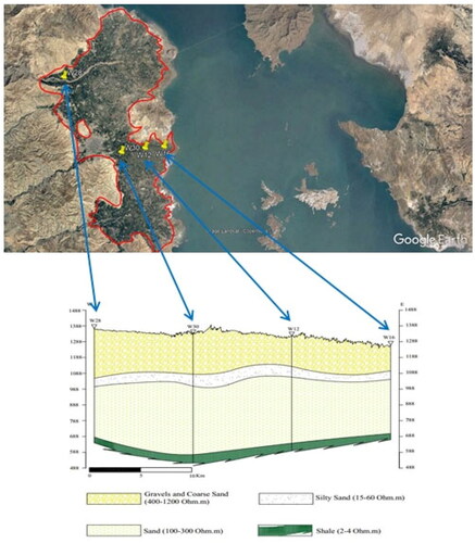
Located at the West Azarbaijan province, Urmia plain has an area of 51762 km² and has been expanded between the geographical coordinates of 44°14′ to 47°53′ east longitude and 35°40′ to 38°30′ north latitude. The research zone is one of the Urmia lake basins covering an area of 2166.2 km² (4.18% of Urmia lake basin area). The shares of plain and mountainous areas are 748.96 and 1249.2 km², respectively. The highest and lowest height of the research zone are 2000 and 1270 m, respectively. Figure 1 displays the location of the study area. A physical and hydrogeological description of the aquifer, including a geological cross section is illustrated in Figure 2.

Figure 1. General location of the study area with geological map and spatial distribution of EC values.

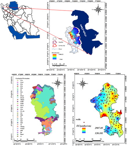
Figure 2. Geological section map of Urmia plain aquifer.

The agricultural section has the highest water consumption of underground water in Urmia plain. The amount of water withdrawal from underground resources was 367.86 Mm³ during 2014–2015. The share of the well and spring were 357.32 and 10.54 Mm³, respectively. The negative value of water balance illustrates the lower inlet water volume than outlet volume. Qualitative data of underground water included measured EC provided with Water Organization of West Azarbaijan. The wells of number 109 were used to compile observed data during 2014–2015. The spatial distribution of measured EC using IDW method has been presented in Figure 1.

2.1.1. The method of modified GALDIT vulnerability assessment

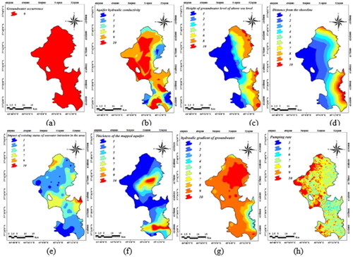
Six intrinsic physical characteristics of the media are included in GALDIT index to provide vulnerability map. The GALDIT is abbreviated from the following six hydrogeological factors: groundwater occurrence (G), groundwater system hydraulic conductivity (A), water table head (L), distance from shoreline (D), impact of present status of saltwater intrusion (I) and saturated media depth (T) (Chachadi and Lobo-Ferreira 2001). This model is utilized for the coastal and Mediterranean zones. The GALDIT approach has been modified by adding a hydraulic gradient map and pumping rate (GALDIT-iP) to provide a precise vulnerability map with maximum conformity with existing conditions to achieve appropriate management options for maintenance and utilization of the Urmia plain aquifer.

The GALDIT method seems to be the only example of a large-scale profiling approach to assess the vulnerability of coastal aquifers to saltwater intrusion. Hence, creating a more flexible method is the aim of the present study. The large population of coastal areas, the increasing demand for fresh water and the prominence of underground water as the main source of water supply in coastal areas have been the reasons for choosing the pumping rate for this research. Obviously, there is a direct relationship between the water level and the amount of pumping. The reason for choosing hydraulic gradient is its decisive role in coastal aquifers as the most important controlling variable of sea water, which provides the main source of groundwater discharge to the sea. On the other hand, the limited data of the water level collected from piezometers and observation wells in some areas and the distribution of wells in a wide range and the accessibility of their statistics compared to the water level, causes more accuracy and confidence in a region. Sometimes, the presence of defects in the piezometer and the network of observation wells causes a deficiency in the measurement of the water level. On the other hand, the large diameter of the pumping wells and the small storage in the well result in misleading water level measurements. Also, in karst systems, their special channel and fissure system cannot represent the real water level. Therefore, in this research, the pumping rate has been introduced to solve the aforementioned problems for measuring the water level.

The map of vulnerability index of GALDIT-iP was obtained in ArcGIS software using Equation (1)(1) $$\text{GALDIT}-\text{iP}\mathrm{ }\text{Index}=\frac{\sum _{\mathrm{i=}1}^8\left(W_i\times R_i\right)}{\sum _{\mathrm{i=}1}^8\left(W_i\right)}\mathrm{ }$$(1) , overlapping of raster layers gotten from parameters from Figure 3 with regards to their order and weighting coefficients. (1) $$\text{GALDIT}-\text{iP}\mathrm{ }\text{Index}=\frac{\sum _{\mathrm{i=}1}^8\left(W_i\times R_i\right)}{\sum _{\mathrm{i=}1}^8\left(W_i\right)}\mathrm{ }$$(1)

Figure 3. (a) Type of aquifer; (b) Hydraulic conductivity map; (c) Level difference map of underground water with sea level; (d) Distance map from the shoreline; (e) Developing map of seawater intrusion; (f) Aquifer thickness map; (g) Hydraulic gradient map, (h): Pumping rate map.

2.1.2. Groundwater occurrence (G)

Seawater intrusion depends on aquifer type. Unconfined, confined and leakage are tree types of aquifers. The highest score belongs to confined one of value 10. The study area is unconfined type based on the Water Organization balance report (Figure 3a).

2.1.3. Aquifer hydraulic conductivity (A)

Hydraulic conductivity is the capability of water transportation through soil or bedrock of aquifer that is created due to the effective porosity of soil particles (Castany 1982). There is a straight relationship between hydraulic conductivity and the penetrability of seawater into the aquifer. The value of hydraulic conductivity was calculated by dividing the transmissivity coefficient by the saturated thickness of the aquifer (Figure 3b).

2.1.4. The difference between underground level and sea level (L)

Level difference plays a significant role to provide required pressure for the movement of seawater into the aquifer. Using Ghyben–Herzberg relationship, for every meter of freshwater withdrawal above the average sea level, the saltwater level rises by 40 m (Figure 3c).

2.1.5. Distance from the shoreline (D)

It is called the air distance between the desired location and the line perpendicular to the shoreline. If the aquifer hydrogeological conditions are susceptible to transfer, it will happen the highest intrusion of seawater into the aquifer when the aquifer distance is short and close to the shoreline (Figure 3d).

2.1.6. Impact of existing status of seawater intrusion in the area (I)

While the amount of bicarbonate in groundwater is much higher than in seawater, the most abundant ion in seawater and the least ion in groundwater is chloride. Equation (2)(2) $$\text{Revelles}\mathrm{ }\text{coefficient}\text{ (I)}=\frac{\left[{\text{Cl}}^{-}\right]}{\left[{\text{HCO}}_3^{-}+{\text{CO}}_3^{2-}\right]}$$(2) has been developed by Revelle (1941) as an index for detecting seawater intrusion into the coastal aquifer and is used as a ranking criterion of the existence of the seawater intrusion effect: (2) $$\text{Revelles}\mathrm{ }\text{coefficient}\text{ (I)}=\frac{\left[{\text{Cl}}^{-}\right]}{\left[{\text{HCO}}_3^{-}+{\text{CO}}_3^{2-}\right]}$$(2)

Figure 3e illustrates the magnitude of the seawater intrusion map.

2.1.7. Thickness of the mapped aquifer (T)

Aquifer thickness has a remarkable role to estimate the amount of seawater into the coastal zone that is called the thickness of the saturation part of the aquifer. The magnitude of seawater intrusion is directly related to the thickness of the aquifer. The thickness of the aquifer is defined as the distance between the water table up to the aquifer impermeable layer (Figure 3f). Table 1 shows the ranking of this parameter.

Table 1. Weights and ratings of the GALDIT and GALDIT-iP parameters (Chachadi 2005; Docheshmeh Gorgij and Asghari Moghaddam 2015).

Aquifer type		Hydraulic conductivity (m/day)		Height of groundwater level of above sea level (m)		Distance from the shoreline (m)
Weight = 1		Weight = 2		Weight = 5		Weight = 3
Range	Rate	Range	Rate	Range	Rate	Range	Rate
Free	9	<1.5	1	8.6–12	10	<1000	10
		1.5–2.5	3	12–17	8	1000–2000	9
		2.5–3.5	5	17–22	6	2000–3000	8
		3.5–6	8	22–27	5	3000–4000	7
		6–10	9	27–32	3	4000–5000	6
		>10	10	32–37	2	5000–6000	5
				37	1	6000–8000	3
						8000–10000	3
						10000-15000	2
						>15000	1
Impact of existing status of seawater intrusion in the area (mEq/L)		Aquifer thickness(m)		Hydraulic gradient		Pumping rates (m^3 per year)
Weight = 6		Weight = 3		Weight = 4		Weight = 4
Range	Rate	Range	Rate	Range	Rate	Range	Rate
<0.1	1	<80	1	<0.003	10	<2000	3
0.1–0.2	3	80–100	3	0.003–0.005	9	2000–5000	5
0.2–0.3	5	100–125	5	0.005–0.007	8	5000–10000	6
0.3–0.5	7	125–150	6	0.007–0.009	7	10000–25000	7
0.5–1	9	150–175	7	0.009–0.01	6	25000–50000	8
>1	10	175–200	8	0.01–0.05	5	50000–100000	9
		200–220	9	0.05–0.1	4	>100000	10
		>220	10	0.1–0.12	3
				0.12–0.14	2
				>0.14	1

2.1.8. Hydraulic gradient (i)

Distance from the shoreline and the level difference of underground water with sea level define the hydraulic gradient. The hydraulic slope of the sea in coastal aquifers provides the main source of groundwater discharge to the sea with overuse of groundwater and the most significant controlling parameter is seawater (Ferguson and Gleeson 2012; Werner et al. 2012; Ketabchi and Ataie-Ashtiani, 2015; Comte et al. 2016; Holding and Allen 2015). Figure 3g displays the map of the hydraulic gradient of the study area.

2.1.9. Pumping rate (P)

The pumping rate can be replaced by the water level in the area of high population and more fresh water consumption which is extracted from underground water resources (Javadi et al. 2012). The pumping wells provide worthy information with the annual pumping rate known due to defects in the network of observation wells in some areas (Figure 3h).

2.2. Genetic algorithm

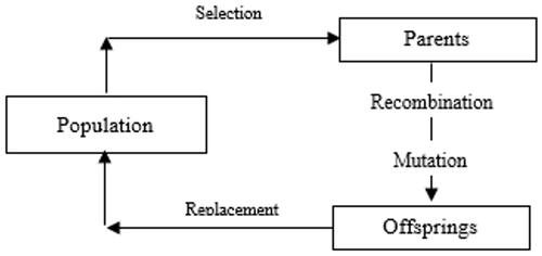
Developed by Holland (1975) and introduced by Goldberg (1989), GA is an evolutionary adaptive method and based on the genetic process of living organisms that is widely used to solve search and optimization problems. The GA is best suited to solve combinatorial optimization problems that cannot be solved using more conventional operational research methods. Hence, it can be applied to large, complex problems that are nonlinear with multiple local optima. In GA, the process starts with a initial population involving set of solutions. Each solution, called chromosome, is encoded in a string. Each chromosome composed of genes which take a quantity of values. First, the population is randomly generated. A new population is then produced at each iteration of generation by employing genetic operators such as mutation, crossover, reproduction and selection. Each solution set is assessed based on a fitness function, and this procedure is stopped when the fitness value reaches a threshold which can be determined by the user. The main aim of the optimization procedure is to minimize or maximize the fitness. Figure 4 illustrates the flowchart of the GA (Savic et al. 1999).

Figure 4. Overview process of the GA.

2.3. Modeling process

A database of EC parameters was provided from observation wells in the study area. Then, the GA was applied to design an optimized monitoring network and determine an efficient wells number and their location.

2.3.1. Database

The number of 109 data were obtained from monitoring wells in the existing study area. The IDW interpolation approach was utilized to extract the raster layer of the study zone. The IDW had the least error and the maximum conformity and correlation than other interpolation methods. The obtained raster layer put EC data into the 741 regular cells with the same distance with mesh size 1000 × 1000 m in the study area.

2.3.2. Optimization model

The defined optimized model follows three objective functions. The first goal illustrates the conformity of the selected monitoring wells with the vulnerability of the modified GALDIT which is obtained from the maximum correlation of vulnerability map and calculated values. The second goal stands for minimizing the number of monitoring wells due to their uneconomical situation. The third target is minimizing the difference between calculated values of EC and measured ones in all aquifer zones using the Nash-Sutcliff index to achieve a precise monitoring network. The equations of the optimization model were defined as follows: (3) $$Z_n\mathrm{ }=\mathrm{ }\max (Z_1\mathrm{ }-\mathrm{ }w{Z}_2\mathrm{ }+\mathrm{ }{Z}_3)\mathrm{ }$$(3) (4) $$Z_1=\frac{\sum _{i=1}^n\mathrm{(}{x}_i-\overline{x}\mathrm{)}\mathrm{(}{y}_i-\overline{y}\mathrm{)}}{\sqrt{\sum _{i=1}^n{\mathrm{(}{x}_i-\overline{x}\mathrm{)}}^2}\mathrm{ }\sqrt{\sum _{\mathrm{i=}1}^n{\mathrm{(}{y}_i-\overline{y}\mathrm{)}}^2}},\mathrm{ }{\mathrm{ }Z}_1\mathrm{ }\mathrm{\in }[-1,1]$$(4) (5) $$Z_2=\frac{n}{m}$$(5) (6) $$Z_3=1-\frac{{\sum }_{i=1}^n{(y_i-y_s)}^2}{{\sum }_{i=1}^n{(y_i-\overline{y_s})}^2}, Z_3 \in [-\infty ,1]$$(6) where x_i is the vulnerability index of point ith, $\overline{x}$ is the mean value of the vulnerability index, y_i is the qualitative parameter at point ith, $\overline{y}$ is the mean value of the qualitative parameter, m and n are number of selected wells via optimization algorithm and the total number of wells at the study zone, respectively; y_s is predicted value of the qualitative parameter and ${\overline{y}}_s$ is the mean value of the qualitative parameter. The Z_n, with the best value +1, is an objective optimization function that changes from −1 to +1 based on three functions Z₁, Z₂ and Z₃ to maximize the correlation between vulnerability index and qualitative parameter of underground water at the first function. Despite the different distinct nature of each three functions, their ideal values equal one; hence the w-weighting coefficient was used in Z_n function for explaining the importance of Z₂ compared to two other functions, that is, Z₁ and Z₃. The different values of the weighting coefficient lead to optimized answers that are calculated using sensitivity analysis of w.

2.3.3. Simulation

The restrictions and the values of objective functions for the optimization problem are determined using simulation. For the first stage, the values of EC are calculated using the layer of the IDW interpolation method all around the study area. Then, the vulnerability index of the calculated points is utilized to compute the value of correlation (Z₁). The Nash-Sutcliff coefficient (Z₃) is computed using interpolated values of EC and measured values of potential database points. Utterly, the values of objective function Z₂ are calculated based on the known number of monitoring wells network.

2.3.4. Optimization process

The crossover probability (P_cross) is utilized for the obtained answers for each step at the GA. High values were assigned to P_cross, that is, between 0.5 and 1, to eliminate repeatable answers. To diversify the number of obtained answers, mutation probability (P_mut) from 0.05 to 0.25 was considered (Fisher, 2013; Ayvaz and Kentel 2015). These phases continue to meet stop conditions. In the present study, a trial and error process was performed using MATLAB software, and the values of population, crossover probability, mutation probability and the maximum values of repetitions were determined as 50, 0.95, 0.05 and 1000, respectively.

3. Results and discussion

3.1. Analysis of the vulnerability map

Data processing was performed in ArcGIS software and the layers of classified vulnerability effective parameters were extracted (Figure 3). Table 1 was utilized for weighting and combination of layers for each parameter; finally, a vulnerability map was provided using Eq. (1)(1) $$\text{GALDIT}-\text{iP}\mathrm{ }\text{Index}=\frac{\sum _{\mathrm{i=}1}^8\left(W_i\times R_i\right)}{\sum _{\mathrm{i=}1}^8\left(W_i\right)}\mathrm{ }$$(1) and overlap of the weighted layers (Figure 5).

Figure 5. The vulnerability map of coastal aquifer of Urmia plain using modified GALDIT-iP.

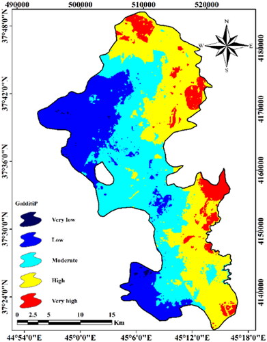
The intended index was illustratively categorized which has been presented in Table 2. The computed values explain the vulnerability of the aquifer relative seawater intrusion so that larger numbers indicate greater aquifer vulnerability. The vulnerability index of the whole plain was estimated between 3 and 8 and was classified in five groups: 3–3.75, 3.75–4.5, 4.5–5.25, 5.25–6 and 6–8. The counterpart vulnerability level for the aforementioned classification was very low, low, average, high and very high, respectively. According to Figure 4, while the northern, central part and coastal margin of Urmia plain have high to very high vulnerability index, in the southern zones and far from the coastal margin, the severity of the vulnerability has decreased.

Table 2. Classification and percentages of vulnerable areas obtained from GALDIT-iP index.

Area (%)	Area (km^2)	Range	Classification
0.02	1.53	3–3.75	Very low
23.80	178.09	3.75–4.5	Low
35.21	263.48	4.5–5.25	Moderate
33.67	251.97	5.25–6	High
7.12	53.32	6–8	Very high
100	748.39	Sum

3.2. Analysis of the GA output

The analysis of the GA is performed based on different W-weighting values (Table 3). According to Table 3, while the objective function was computed as 1.927 for W = 0.01 with correlation coefficient 0.952 and Nash-Sutcliff coefficient 0.978, the number of monitoring wells was determined as 234. It has 125 wells more than the exiting monitoring network. The value of the objective function was computed as 1.887 for W = 0.2, with the maximum values of Nash-Sutcliff function of 0.9843 and well numbers of 178 (69 wells more than the existing monitoring network). Using 91 wells with a correlation coefficient of 0.935 and Nash-Sutcliff of 0.979, the value of the objective function was calculated as 1.791 for W = 1.0. The number of wells decreased from 109 to 91. There is no significant difference between well number at the monitoring network for a tenfold increase in weight (W = 1 and W = 10). But a remarkable decrease is recognizable for a tenfold rise from W = 0.1 to W = 1.0. Although the objective function Z_n changes from 1.791 to −99.617 (a distinguishing difference) for W = 1 to W = 1000, the difference in the number of selected wells is not large. The lowest well number relates to W = 1000, but this does not meet the best answer because the values of functions Z₁ and Z₃ determine various locations for wells that optimize the final objective function. Also, for similar values of W, the less vales of the wells number, has a more negative effect on the Z₂ and Z₃. Hence, the optimization model during the optimization process tends to keep the wells number constant and search for better well positions to modify the values of Z₁ and Z₃. There is no more difference between well number for W = 1 and W = 10, but according to the final objective function and various Z₁ and Z₃ functions for these two weights, different locations are obtained for opted wells with a very impressive ultimate result.

Table 3. Results obtained for different w values.

Weighting coefficient (w)	Correlation between EC and vulnerability (Z1)	Ratio between the number of all available monitoring wells and selected wells (Z2)	NS model efficiency (Z3)	Objective function (Zn)	Number of selected wells (n)
0.01	0.952	0.316	0.978	1.927	234
0.1	0.942	0.270	0.9841	1.899	200
0.2	0.950	0.240	0.9843	1.887	178
0.3	0.951	0.206	0.978	1.867	153
0.4	0.948	0.182	0.974	1.849	135
0.5	0.938	0.188	0.966	1.810	139
0.6	0.939	0.167	0.971	1.810	124
0.7	0.940	0.135	0.979	1.824	100
0.8	0.942	0.126	0.980	1.822	93
0.9	0.918	0.142	0.971	1.762	105
1	0.935	0.123	0.979	1.791	91
10	0.792	0.113	0.964	0.622	84
100	0.621	0.074	0.894	−5.907	55
1000	0.650	0.101	0.948	−99.617	75

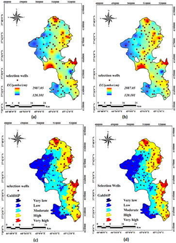
Figure 5 presents the conformity of the vulnerability map and interpolated map of EC values along with proposed locations of wells for W = 1 and W = 10. The spatial distribution of wells reveals that the location of proposed wells has been located in regions with critical values in terms of vulnerability and EC. A comparison of the spatial distribution of monitoring wells according to the raster map of the presented EC values and the optimized situation in Figure 6 shows that in areas where aquifer salinity is higher and conditions are more critical, the number of selected wells is higher than the current situation and on the contrary in areas that are less at risk, the number of selected wells is less than the current situation. It can be concluded that although the wells number is less in W = 10 and is more economical, according to the comparison of selected locations, the accuracy of the selected positions is higher for W = 1.0. According to the optimization model, it can be claimed that the ultimate monitoring network is opted by examining the appropriate weight, optimal wells number and correct spatial distribution of wells. Less wells number for high weighting is economical but the accuracy of qualitative results declines due to the reduction of correlation function (Z₁) and Nash-Sutcliff function (Z₃).

Figure 6. Interpolation map of EC matching for (a) w = 1 and (b) w = 10 and vulnerability map matching for (c) w = 1 and (d) w = 10.

3.3. Results verification

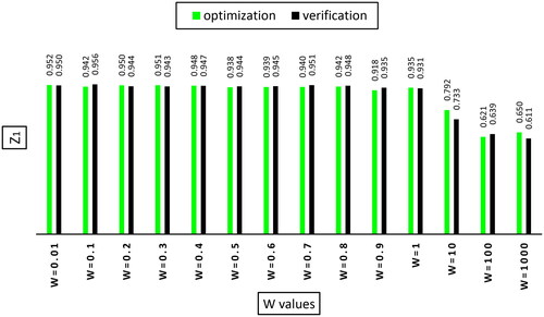
The verification of the results can be assessed for the accuracy of the monitoring network for various time series. In the present study, the values of EC in 2016 were used to verify the monitoring network extracted from 2015. Figure 7 illustrates the verification of the results using the correlation coefficient. The values of the correlation coefficients for W = 0.1, 0.5, 0.6, 0.7, 0.8, 0.9 and 100 during verification period are higher than the optimization period, indicating results precisely.

Figure 7. Validation of correlation coefficient of optimal wells for different w values.

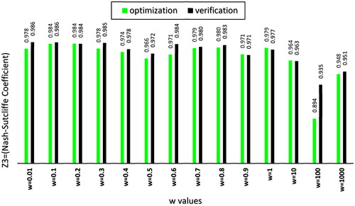
Verification of results in terms of the Nash-Sutcliff coefficient for 2015 and 2016 is shown in Figure 8. Moriasi et al. (2007) presented the following classification of Nash-Sutcliff coefficient: 0.75–1 (very good), 0.65 − 0.75 (good), 0.5–0.65 (acceptable), <0.5 (unacceptable). According to Figure 8, all weights are included in the very good category.

Figure 8. Validation of Nash-Sutcliffe coefficient model of optimal wells for different w values.

The values of root mean square error (RMSE), bias percent (PBIAS) and standard deviation (S) are calculated using the following equations: $$\text{RMSE}=\sqrt{\frac{1}{n}\sum _{i=1}^n{(y_s-y_i)}^2}$$ (7) (8) $$\text{PBIAS}=\frac{{\sum }_{i=1}^n(y_i-y_s)}{{\sum }_{i=1}^n{y}_i}\times 100$$(8) (9) $$S=\sqrt{\frac{1}{n-1}\sum _{i=1}^n{(y_s-\overline{y}{ }_s)}^2}$$(9) where n is the number of selected wells, y_i is the value of the qualitative parameter at the point ith, y_s is the predicted value of the qualitative parameter, ${\overline{y}}_s$ is the mean value of the qualitative parameter. The results of Eqs. (7)(7) to (9)(9) $$S=\sqrt{\frac{1}{n-1}\sum _{i=1}^n{(y_s-\overline{y}{ }_s)}^2}$$(9) have been presented in Table 4. Singh et al. (2004) named an answer as a solution with less error if the value of the RMSE is less than half of S. For all the data in Table 4, both verification and optimization periods for all weights have above-mentioned condition. Santhi et al. (2001) and Van Liew et al. (2003) claimed that the values of r(Z₁) more than 0.5 are acceptable. Thus, all weights in Table 4 are allowable precise. PBIAS index shows the average deviation of the predicted values from the observed values in terms of percentage. The closer the value of PBIAS to zero indicates less difference and more accurate answer. Moriasi et al. (2007) classified PBIAS values less than 10% as very good estimations.

Table 4. Validation outcomes for different weights w values.

Weighting coefficient (w)	Optimization (95)				Verification (97)
	PBIAS	RMSE	S	r	PBIAS	RMSE	S	r
0.01	0.321	57.135	372.436	0.952	0.264	38.817	319.889	0.950
0.1	−0.157	47.247	361.662	0.942	−0.311	42.477	348.019	0.956
0.2	−0.245	48.720	380.588	0.950	−0.147	44.996	347.443	0.944
0.3	0.081	58.549	383.133	0.951	0.111	42.915	345.195	0.943
0.4	0.591	60.960	355.856	0.948	0.444	54.813	349.155	0.947
0.5	1.434	78.075	386.651	0.938	1.222	67.673	376.868	0.944
0.6	0.010	69.783	378.327	0.939	0.051	47.316	357.660	0.945
0.7	1.081	60.781	400.752	0.940	1.051	52.351	356.711	0.951
0.8	−0.453	62.094	415.268	0.942	−0.110	47.886	353.136	0.948
0.9	1.345	76.572	419.738	0.918	1.348	70.837	371.356	0.935
1	1.073	77.892	350.813	0.935	0.851	54.369	335.073	0.931
10	−0.892	56.885	282.989	0.792	−0.756	58.791	285.260	0.733
100	−1.044	103.770	282.988	0.621	−1.093	78.328	285.644	0.639
1000	0.979	80.598	327.554	0.650	0.911	68.216	267.619	0.611

Table 5 shows the changes of mean EC values for various weights during optimization and the existing monitoring network. According to Table 5, there is an adverse relationship between different weights and wells number so that the decrease in the number of monitoring wells corresponds to the increase in the EC average. In other words, the optimization model firstly opts for high values of EC and the maximum correlation coefficient with vulnerability index; then the points of low values of EC and correlation coefficient are chosen. Therefore, it is better to choose a weight with high average values of EC.

Table 5. The change of mean EC values in monitored groundwater quality (unit: µSiemens/cm).

Year:1395	Without optimization	With optimization
W	–	0.01	0.1	0.5	1	10	100	1000
n	n = 109	234	200	139	91	84	55	75
Mean EC	929.633	865.872	867.205	876.418	1043.830	901.631	909.580	937.400

4. Conclusion

Inappropriate spatial distribution of monitoring wells is one of the fundamental issues for monitoring networks. Incorrect results are obtained due to incomplete information in critical points and/or excess information in non-critical points because of monitoring wells distribution. Also, the extra number of monitoring wells is not economically viable. The optimization process is known as an appropriate solution for designing a monitoring network. The mission of the present study is designing an optimized monitoring network at the study area. The time-series 2015 and 2016 were used for optimization and verification processes, respectively. GALDIT-IP index was developed and utilized to obtain vulnerability map of the plain.

Increasing correleation coefficient from 0.42 to 0.66 demonstrated the admissible correction of the new monitoring network. The economical objective function was applied at the main objective function to obtain optimal answers based on the direct relationship between wells number and the cost of monitoring network design. The number of wells was reduced by 17% in the presented study. Jason (2013), Mahmoudpour et al. (2021) and Sadatinejad et al. (2019) performed an analysis using the GA method to optimize well numbers. Their results led to reduction of well numbers besides acceptable precision. The application of three targets into the one objective function using w-weighting coefficients illustrated the relative importance of goals. The results of optimization evaluation in different weights showed the importance of w in determining the optimal solution. The value of w should be opted based on the most optimized answer with the most appropriate relationship among all objective functions. RMSE, PBIAS and standard deviation were utilized to determine the optimal solution. Utterly, a comparison between mean values of computed and measured EC was used to identify more pollutant areas. From this study, the following conclusions can be reached:

• Based on the different weights of W, the results of the genetic algorithm were analyzed. Choosing the optimal solution highly depends on the weighting factor W. Therefore, the value of W should be chosen according to the most balanced solution. The most balanced and optimal solution means an acceptable relationship between the cost and the spatial distribution of wells in the region. Different weights lead to the creation of different optimal quality monitoring networks.

• In order to design the spatial distribution of monitoring wells, it is better to choose important and critical areas such as points with poorer quality, because these data better reflect the quality of underground water in more polluted areas.

• The design of the underground water quality monitoring network should be periodically optimized because the successive evaluations of the monitoring network play an important role in determining the long-term evaluation of the underground water quality and the factors affecting it. This can be of great help in planning and applying methods to improve the quality of underground water.

Disclosure Statement

No potential conflict of interest was reported by the author(s).

References

- Aller L, Bennett T, Lehr JH, Petty RJ, Hackett G. 1987. DRASTIC: a standardized system for evaluating groundwater pollution using hydrogeologic settings. EPA, 600/2-87-035.
- Ayvaz MT, Elçi A. 2018. Identification of the optimum groundwater quality monitoring network using a genetic algorithm based optimization approach. J Hydrol. 563:1078–1091.
- Ayvaz MT, Kentel E. 2015. Identification of the best booster station network for a water distribution system. J Water Resour Plann Manage. 141(5):4014–4076.
- Baalousha H. 2010. Assessment of a groundwater quality monitoring network using vulnerability mapping and geostatistics: a case study from Heretaunga Plains, New Zealand. Agric Water Manag. 97(2):240–246.
- Babiker IS, Mohamed AA, Hiyama T, Kato K. 2005. A GIS-based DRASTIC model for assessing aquifer vulnerability in Kakamigahara Heights, Gifu Prefecture, central Japan. Sci Total Environ. 345(1–3):127–140.
- Barbash JE, Resek EA. 1996. Pesticides in ground water: distribution, trends, and governing factors. Chelsea: MI7 Ann Arbor Press.
- Barzegar R, Razzagh S, Quilty J, Adamowski J, Kheyrollah Pour H, Booij MJ. 2021. Improving GALDIT-based groundwater vulnerability predictive mapping using coupled resampling algorithms and machine learning models. J Hydrol. 598:126370.
- Bordbar M, Khosravi K, Murgulet D, Tsai FT-C, Golkarian A. 2022. The use of hybrid machine learning models for improving the GALDIT model for coastal aquifer vulnerability mapping. Environ Earth Sci. 81(15):402.
- Bordbar M, Neshat A, Javadi S. 2018. Vulnerability assessment of Gharesou-Gorganroud coastal aquifer using GALDIT and SINTACS and optimization by SPSA and GIS. Iran J Eco Hydrol. 5(2):699–711.
- Bordbar M, Neshat A, Javadi S. 2019. Using Fuzzy logic and AHP models to modify GALDIT model in coastal aquifer vulnerability assessment. Iran Water Resour Res. 15(1):314–326.
- Castany G. 1982. Principes et methods de l hydrogeologie. Paris: Dunod, p. 236.
- Chachadi AG. 2005. Seawater intrusion mapping using modified GALDIT indicator model-case study in Goa. Jalvigyan Sameeksha. 20:29–45.
- Chachadi AG, Lobo-Ferreira JP. 2001. Seawater intrusion vulnerability mapping of aquifers using the GALDIT method. Coastin. 4:7–9.
- Chadalavada S, Datta B. 2008. Dynamic optimal monitoring network design for transient transport of pollutants in groundwater aquifers. Water Resour Manage. 22(6):651–670.
- Comte J-C, Cassidy R, Obando J, Robins N, Ibrahim K, Melchioly S, Mjemah I, Shauri H, Bourhane A, Mohamed I, et al. 2016. Challenges in groundwater resource management in coastal aquifers of East Africa. J Hydrol Reg Stud. 5:179–199.
- Dhar A, Patil RS. 2012. Multiobjective designof groundwater monitoring network underepistemic uncertainty. Water Resour Manage. 26(7):1809–1825.
- Docheshmeh Gorgij A, Asghari Moghaddam A. 2015. Vulnerability assessment of saltwater intrusion using simplified GAPDIT Method: a case study of Azarshahr Plain Aquifer, East Azerbaijan, Iran.
- Doerfliger N, Jeannin PY, Zwahlen F. 1999. Water vulnerability assessment in karst environments: a new method of defining protection areas using a multiattribute approach and GIS tools (EPIK method). Environ Geol. 39(2):165–176.
- Ferguson G, Gleeson T. 2012. Vulnerability of coastal aquifers to groundwater use and climate change. Nat Clim Change. 2(5):342–345.
- Foster S. 1987. Fundamental concepts in aquifer vulnerability, pollution risk and protection strategy. International Conference, the Netherlands Vulnerability of Soil and Groundwater to Pollutants. Netherlands Organization for Applied Scientific Research. The Hague, vol. 38, p. 69–86.
- Goldberg DE. 1989. Genetic algorithms in search, optimization, and machine learning. Boston, MA: Addison Wesley Longman Publishing Co., Inc.
- Gontara M, Allouche N, Jmal I, Bour S. 2016. Sensitivity analysis for the GALDIT method based on the assessment of vulnerability to pollution in the northern Sfax coastal aquifer, Tunisia. Arab J Geosci. 9:416.
- Holding S, Allen DM. 2015. numerical modeling of freshwater lens response to climate change stressors on small islands. Hydrol Earth Syst Sci. 19(2):933–949.
- Holland JH. 1975. Adaptation in natural and artificial systems; MIT Press: Cambridge, MA, USA.
- Jason CF. 2013. Optimization of Water-Level Monitoring Networks in the Eastern Snak River Plain Aquifer Using a Kriging-BasedGenetic Algorithm Method. Prepared incooperation with the Bureau of Reclamation and U.S. Department of Energy, USGS.
- Javadi AA, Abd‐Elhamid HF, Farmani R. 2012. A simulation optimization model to control seawater intrusion in coastal aquifers using abstraction/recharge wells. Int J Numer Anal Meth Geomech. 36(16):1757–1779.
- Kallioras A, Pliakas F, Skias S, Gkiougkis I. 2011. Groundwater vulnerability assessment at SW Rhodope aquifer system in NE Greece. Adv Res Aquat Environ. 2:351–358.
- Kanani TJ, Malek AM, Prakash I, Mehmood K. 2017. Ground water vulnerability assessment of coastal area of Porbandar, Gujarat, India. Int J Sci Res Dev. 5:796–799.
- Kardan Moghaddam H, Javadi S. 2016. Evaluation vulnerability coastal aquifer by GALDIT index and calibration by AHP method. Water Soil Conserv. 23(2):163–177.
- Ketabchi H, Ataie-Ashtiani B. 2015. Coastal groundwater optimization—advances, challenges, and practical solutions. Hydrogeol J. 23(6):1129–1154.
- Khader A, McKee M. 2014. Use of a relevance vector machine for groundwater quality monitoring network design under uncertainty. Environ Modell Softw. 57:115–126.
- Kura NU, Ramli MF, Ibrahim S, Sulaiman WN, Aris AZ, Tanko AI, Zaudi MA. 2015. Assessment of groundwater vulnerability to anthropogenic pollution and seawater intrusion in a small tropical island using index-based methods. Environ Sci Pollut Res Int. 22(2):1512–1533.
- Lobo-Ferreira JP, Chachadi Diamantino AGC, Henriques MJ. 2005. Assessing aquifer vulnerability to seawater intrusion using GALDIT method: part 1-Application to the Portuguese Aquifer of Monte Gordo. The Forth Inter-Celetic Colloquium on the Hydrology and Management of Water Resources, Guimaraes, Portugal: p. 1–12.
- Luo Q, Wu J, Yang Y, Qian J, Wu J. 2016. Multiobjective optimization of long-term groundwater monitoring network design using a probabilistic Pareto genetic algorithm under uncertainty. J Hydrol. 534:352–363.
- Luoma S, Okkonen J, Korkka-Niemi K. 2017. Comparison of the AVI, modified SINTACS and GALDIT vulnerability methods under future climate change scenarios for a shallow low-lying coastal aquifer in southern Finland. Hydrogeol J. 25(1):203–222.
- Mahmoudpour H, Janatrostami S, Ashrafzadeh A. 2021. Design of the optimal groundwater quality monitoring network using the aquifer vulnerability map. Iran-Water Resour Res. 16(4):154–173.
- Moriasi DN, Arnold JG, Van Liew MW, Bingner RL, Harmel RD, Veith TL. 2007. Model evaluation guidelines for systematic quantification of accuracy in watershed simulations. Am Soc Agric Biol Eng. 50(3):885–900.
- Nadjla B, Abdellatif D, Assia S. 2021. Mapping of the groundwater vulnerability to saline intrusion using the modified GALDIT model (Case: the Ain Temouchent coastal aquifer, (North-Western Algeria)). Environ Earth Sci. 80(8):319.
- Nakhaei M, Mohammadi M, Rezaei M. 2014. Optimizing of aquifer withdrawal numerical model using Genetic Algorithm (Case Study: Uromiyeh Coastal Aquifer). Iran-Water Resour Res. 10(2):94–97.
- Nakhaei M, Vadiati M, Mohammadi K. 2015. Evaluation of vulnerability of Urmia Lake Saline Water intrusion to coastal aquifer using GALDIT model. Geosci Sci Q J. 24(95):223.
- Pedreira R, Kallioras A, Pliakas F, Gkiougkis I, Schuth C. 2015. Groundwater vulnerability assessment of a coastal aquifer system at River Nestos eastern Delta, Greece. Environ Earth Sci. 73(10):6387–6415.
- Revelle R. 1941. Criteria for recognition of sea water in ground waters. Trans AGU. 22(3):593–597.
- Sadatinejad SJ, Ghasemi L, Yousefi H. 2019. Redesign of groundwater monitoring network Kuhdasht aquifer. Iran J Eco-Hydrol. 5(4):1255–1266.
- Santha Sophiya M, Syed TH. 2013. Assessment of vulnerability to seawater intrusion and potential remediation measures for coastal aquifers: a case study from eastern India. Environ Earth Sci. 70(3):1197–1209.
- Santhi C, Arnold JG, Williams JR, Dugas WA, Srinivasan R, Hauck LM. 2001. Validation of the SWAT model on a large river basin with point and nonpoint sources. J Am Water Resourc Assoc. 37(5):1169–1188.
- Savic DA, Evans KE, Silberhorn T. 1999. A Genetic Algorithm–Based System for the Optimal Design of Laminates. Computer Aided Civil Infrastructure Engg. 14(3):187–197.
- Singh J, Knapp HV, Demissie M. 2004. Hydrologic modeling of the Iroquois River watershed using HSPF and SWAT. ISWS CR 2004-08. Champaign, Ill: Illinois State Water Survey.
- Tasnim Z, Tahsin S. 2016. Application of the method of Galdit for groundwater vulnerability assessment: a case of south Florida. Asian J Appl Sci Eng. 5:27–40.
- Tesoriero AJ, Inkpen EL, Voss FD. 1998. Assessing groundwater vulnerability using logistic regression. Proceedings for the Source Water Assessment and Protection 98 Conference, Dallas, TX, p. 157–165.
- Thapinta A, Hudak PF. 2003. Use of geographic information systems for assessing groundwater pollution potential by pesticides in Central Thailand. Environ Int. 29(1):87–93.
- Trabelsi N, Triki I, Hentati I, Zairi M. 2016. Aquifer vulnerability and seawater intrusion risk using GALDIT, GQISWI and GIS: case of a coastal aquifer in Tunisia. Environ Earth Sci. 75(8):669–710.
- Van Liew MW, Arnold JG, Garbrecht JD. 2003. Hydrologic simulation on agricultural watersheds: choosing between models. Trans ASAE. 46:1539–1551.
- Vrba J, Zaporozec A. 1994. Guidebook on mapping groundwater vulnerability. In International Contributions to Hydrology. Hannover: Heinz Heise.
- Werner AD, Ward JD, Morgan LK, Simmons CT, Robinson NI, Teubner MD. 2012. Vulnerability indicators of sea water intrusion. Ground Water. 50(1):48–58.
- Yang XS, Gandomi AH, Talatahari S, Alavi AH. 2012. Geotechnical and transport engineering. In Metaheuristics in water. 1st ed. Amsterdam: Elsevier.
- Yang JS, Jeong YW, Agossou A, Sohn JS, Lee JB. 2022. GALDIT modification for seasonal seawater intrusion mapping using multi criteria decision making methods. Water. 14(14):2258.