Impact of climate change on hydrological response of Mojo river catchment, Awash river basin, Ethiopia

Abstract

Climate change is a change in the state of climate identified by a change in temperature and precipitation that affect the hydrology of basins. This study has investigated the effects of climate change on the stream flow of Mojo River Catchment using (CORDEX)-Africa data outputs under RCP4.5 and RCP8.5 scenarios. Three-time horizons: near period (2006–2031), mid-period (2031–2055), and far period (2056–2080) were used. The SWAT model was used to simulate runoff. From the MIROC-MIROC5 Model result, the mean annual precipitation is increasing under RCP4.5 and decreasing under RCP 8.5. Similarly, the mean annual temperature shows an increasing trend for both scenarios. The mean annual streamflow shows a decreasing trend in the near and mid-future under both scenarios and only increases (by 6.31 m³/s) in the far future under RCP8.5. For MPI-M-MPI-ESM-LR, the mean annual precipitation shows a decreasing trend under RCP 4.5 and increasing under RCP 8.5, but the mean annual temperature becomes increasing for both scenarios. However, streamflow shows an increase under both scenarios in the all-time horizons and decreases (by 6.68 m³/s) under RCP 8.5 in the near and mid-future. The result of this study indicates that climate change affects streamflow. Therefore, different water-based design operations should incorporate climate change scenarios.

Keywords:

• Climate change
• GCM
• Mojo River
• RCP
• SWAT

1. Introduction

Water is a mobile resource it falls from the clouds, seeps into the soil, flows through aquifers, runs along with stream courses, and eventually backs to the cloud. All life forms and nature’s economy are based on this natural cycle (Rahmato 1999). But any type of management that disrupts the natural cycle comes at a cost, not just financially but in terms of environmental damage and increased health risks.

Climate change impact studies associated with global warming as a result of an increase in greenhouse gases (GHG) has been given ample attention worldwide in recent decades (Papadimitriou 2004; Dodman 2009). Climate Change to future projections temperature will increase by 1–2$°\mathrm{C}$ over eastern Africa in the coming century (Jaramillo et al. 2011), and also many river basins are at risk in sub-Saharan Africa as well. These basins are sensitive to future climate change and the highly variable climate system, as well as poor management and high level of poverty in the population limit the efforts to adapt to climate change (Cooper et al. 2008). The advancements in climate models have increased confidence in the outputs required as inputs for hydrological applications (Wood et al. 2004). However, hydrological impact studies ought to receive more attention as there are still grey areas (areas of activity not readily conforming to climate change) related to the interfacing of climate and hydrological models. Vulnerable hydrological resources are too important to defer climate change investigations (M. T. Taye et al. 2011).

Hailemariam (1999) create better awareness of the effects of climate change on the water resources of the Awash River Basin. A temperature increase of 2.4 and 3.0 °C, respectively, was projected by models for a doubling of CO₂. Therefore, the Awash River Basin would be significantly affected by the changing climate since then; for instance, Taye (2018) and Daba (2015) indicate that the projections for the future period show an increase in water deficiency in all seasons and for parts of the basin, due to a projected increase in temperature and decrease in precipitation. This decrease in water availability will increase water stress in the basin. In Ethiopia, most climate change impact studies on water resources focus on catchments of the Nile basin, for instance (Conway 1997; Alemseged and Tom 2015; Worku et al. 2018).

Trend analysis of the annual rainfall showed there was a declining trend in the northern half of the country and southern Ethiopia while there is an increasing trend in the central part of the country (Cheung et al. 2008). Associated with rainfall and temperature change and variability, there were recurrent drought and flood events in the country. There was also an observation of water level rise and dry-up of lakes in some parts of the region depending on the general trend of the temperature and rainfall pattern of the regions (Abraham et al. 2006).

The Awash River basin, in Ethiopia, is subject to high climate variability, experiencing frequent floods and droughts. The basin is already subject to water stress, with higher water demand than supply (Adeba et al. 2016). Most of the stations in the Mojo watershed showed low variation in annual rainfall (CV%) while the main (Kiremt) and short (Belg) season rainfall exhibited CV ranging from low to high. Both annual and seasonal rainfall showed a non-significant trend at all stations for the past 30 years. However, the majority of stations showed an increasing trend in annual daily average temperature ranging from 0.2 to 0.6 °C per decade (Eshetu 2020). The temperature decline in stream flow at Modjo watershed could likely affect the downstream Koka dam water reserve. Another important potential concern of climate change is hydrological component alteration and subsequent changes in river Hydrology (Girma 2013). The catchment contributes water for irrigation for the society nearby the river and the Rapid growth of agriculture, industries, and urbanization within the catchment become increased recently (Eshetu 2020).

The majority of research on the impact of climate change on hydrological response specifically, precipitation and temperature variation on stream flow in the Awash basin studies are limited. Even, those studies focused on the performance of the models overall the basin using monthly data for instance (Worku et al. 2018; Taye et al. 2018) and on the other hand some the scholars forces on the Upper Awash River Basin is located in Central Ethiopia (Getahun et al. 2014; Emiru et al. 2021). The study by (Bekele et al. 2019) found increasing runoff projection in the 2050s whereas (Daba 2015) found decreasing streamflow projection. These results can partly contribute to the differences in climate models used in the analysis. Similarly, In the watershed, there is a relative lack of studies and consistent daily data Modeled projections on the impact on stream flow at the catchment level. The climate models’ geographic area is found to be the major source of uncertainty (Emiru et al. 2021), and selecting the best models that are better suited for the area under study is essential to deliver robust findings which is critically effected by sediment accumulation in Mojo Catchment for (Gonfa and Kumar 2015, 2016). Most of the studies in Awash basin has been conducted using a single scenario (RCP8.5).

Therefore, an attempt has been made in this study to assess the impact of climate change on hydrologic responses and identify daily frequency using a suitable model at this catchment level to take the effect into account by the policy and decision-makers when planning water resources management. This study examines the pattern of hydrological change and determines the pattern of climate change with its impact on the Mojo catchment. This study aims to quantify the possible climate change impact on the streamflow with different periods using GCMs CORDEX-Africa Models with RCP 4.5 and 8.5 scenarios. This is the main objective of the study because the Mojo River catchment is more important for the socio-economic activity of the community around the catchment. Hence hydrology of the catchment incorporating climate change is assessed to cope up with the impact.

2. Materials and methods

2.1. Description of the study area

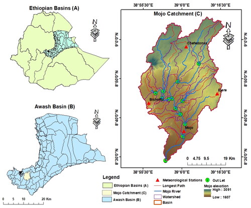
There are around 12 basins in Ethiopia (African Region) (Figure 1A). The awash basin is one of the basins in which our study area exists (Figure 1B). Mojo River catchment (Figure 1C) is mainly located in the Awash basin, with a geographical location between 38⁰54′22′′ to 39⁰17′18′′E and 08⁰24′15′′ to 09⁰07′49′′N and an elevation between 1607 and 3091 meters above sea level. Mojo river is a perennial river that flows through, the town of Mojo located some 43 km southeast of the capital Addis Ababa. It is a tributary of the Awash River receiving effluents. In addition, extensive agricultural practices and human settlements have been altering the catchment and riparian zone of the Mojo River. The catchment covers a surface area of 1601.84 km² (Figure 1).

Figure 1. Location map of Mojo Catchment: (A) Ethiopian basins, (B) Awash Basin, and (C) Mojo catchment.

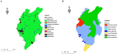
According to the Ethiopian Ministry of Water and Energy the dominant soil types identified in the Mojo catchment includes Eutric Vertisoils, Vertic cambisols, Haplic Luvisols, Luvic Phaeozems, and Lithic Leptosols covers, Chromic lavisols and Mollic Andosols which is extracted from Awash basin soil map. And the dominant land use type in the Mojo catchment is rainfed agricultural land (Figure 2B). According to the Oromiya Region water and design office Land cover classification, the major land use found in the catchment areas are Agriculture, settlement, waterbody, sugarcane plantation, and others available in the catchment (Figure 2A).

Figure 2. Mojo Catchment Land use map (A) and soil type (B) (Source: Oromiya Region water and design office and Ethiopian Ministry of Water and Energy, respectively).

The majority of the catchment particularly the central and lower part of the catchment has a monomodal rainfall pattern whereas the upper part of the catchment is characterized as bimodal. More than 80% of the annual rainfall is received from June to September (locally known as Kiremt) whereas the short season extends from February/March to May (locally known as Belg) (Gonfa and Kumar, 2016). and reported exhibiting most rainfall occurring between June and October thirty years from (1980 to 2005) rainfall records over 4 stations within and adjacent to the study area show an average annual rainfall between 980.8 mm and 913 mm with a mean annual value of 947.3 mm of air temperature that averaged 20.40 $°\mathrm{C}$ varying between a minimum of 11.6$°\mathrm{C}$ in August and a maximum of 29.20$°\mathrm{C}$ in May, with average annual temperature decreasing with an increase in altitude.

The Mojo catchment and its tributaries are a perennial source of water in the study area. The total annual mean flow of the catchment is 214.55 m³/s. Mojo River, which joins lake Koka from the north, the storage mainly fed during the wet season from June to September. After being released through the dam the Awash descends into the Rift Valley northwest towards Awash Station from where the river follows the valley northwards into Gedebassa Swamp near Hertale (Gudeta et al. 2022).

3. Methodology

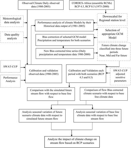
The general methodology used in this study is well presented in the flow chart (Figure 3).

Figure 3. Flow chart of the study.

3.1. Data availability and precipitation and temperature scenarios data collection

Climate change projections involve uncertainties due to various assumptions in GCM conceptualizations, and scenario developments (IPCC 2014). Due to such uncertainties, multiple GCM outputs and scenarios are often used to get plausible estimates of the future climate (Christensen and Christensen 2007). Ongoma et al. (2019) evaluated 22 CMIP5-GCMs for historical simulations of precipitation for East Africa, and Taye (2018) estimates the climate change on water availability in the Awash basin based on the most regionally representative climate models. But both authors estimate GCMs models based on the monthly frequency data. So, identification and estimation of daily hydrological data (temperature and precipitation) are essential for this study area for a precise result. The data needed for climate change analysis is available on the website of (https://esgf-node.llnl.gov/projects/esgf-llnl/) portal. Table 1 shows the candidate models download to analyze the impact of climate change.

Table 1. Candidate GCM models.

Global Climate Models (GCM)	Regional Climate Models
CCCma-CanESM2	RCA4
IPSL-IPSL-CM5A-MR	RCA4
MIROC-MIROC5	RCA4
MPI-M-MPI-ESM-LR	RCA4

The daily precipitation, temperature maximum, and minimum from 1980 to 2100 were extracted from grid cells covering the Mojo catchment. The period from 1980 to 2005 was considered the historical period, based on the good quality of observational climatic data, and hydrological data were used for model calibration and validation. In this study, the period 1981–2005 is used as the historical reference period and three-time slices are used for the future: Near future (2006–2030), mid-future (2031–2055), and far future (2056–2080).

3.2. Selection of RCPs

RCPs are time- and space-dependent trajectories of greenhouse gas and pollutant concentrations and emissions resulting from human activities, such as land use change. According to IPCC (2014) report, four Emission scenarios (i.e. RCP2.6, RCP4.5, RCP6, and RCP8.5) are available. However, only emission scenarios RCP 4.5 and RCP 8.5 are used. Because emission scenarios RCP4.5 mid-range and RCP 8.5 high-level climate scenarios with assumed stabilization radiative forcing to 4.5 and 8.5 W/m² by 2100, respectively, were expected to capture a reasonable range in climatic, and hydrological projections. The high emission scenario (RCP8.5: Moss et al. 2010) and a moderate emission scenario (RCP4.5: Thomson et al. 2011) were chosen for this study. Those candidate GCMs (Table 1) filtered based on the project CORDEX-Africa (AFR-44) as experimental data which is historical, RCP 4.5 and RCP 8.5 of daily data scenarios, the time-frequency is daily data, Regional Climate Model (RCM) is RCA4, four different GCMs and the institute which is data available in SMHI (Table 2).

Table 2. Features of selected GCM models.

Model selection criteria	Variables
Project	CORDEX
Institute	SMHI
Experiment	Historical, RCP 4.5, and 8.5
Ensemble	r1i1p1
Variable	pr, Tmax, tmin
Time-frequency	Daily
Regional climate model (RCM)	RCA4
Domain	AFR-44

Where r1i1p1, which represents realization #1, initialization I #1, and physics p #1; SMHI: Swedish Meteorological and Hydrological Institute; RCA4: Rossby Centre; pr: precipitation; Tmax: maximum temperature; Tmin: minimum temperature.

3.3. Bias correction method

Bias correction methods that can better transfer the observed precipitation and temperature statistics to the raw ensemble GCM/RCM CORDEX-Africa RCP 4.5 and RCP 8.5 climate scenarios. In a bias correction of precipitation data, the quantile mapping (QM), the detrended quantile mapping (DQM), and the quantile delta mapping (QDM) methods have been widely employed because they can correct biases considering high order moments (Seo and Kim 2018). Additionally, these methods were designed to preserve long-term changes in quantiles projected by climate models (Seo and Kim 2018). Thus, the QM-based bias correction method is employed for precipitation correction in this study. (1) $$Q_m\left(t\right)=\{\begin{array}{c}{F}_o^{-1}\left[F_s\left[Q_s\left(t\right)\right]\right], Q_s\ge Q_{th}\\ 0, {\mathrm{ }Q}_s\le Q_{th}\end{array}$$(1) where $Q_m(t)$ and $Q_s\left(t\right)$ are tth bias-corrected data and simulated data from the RCM during the reference period (also known as the historical period), F_s and $F_o^{-1}$ are the cumulative distribution function (CDF) of the raw data from the RCM and the inverse CDF of the observed data, respectively. To categorize between the wet and the dry day threshold value $Q$ (observed) is used (the day with precipitation greater than 1 mm is assumed to be a wet day). The temperature is corrected using Normal Distribution Quantile mapping. (2) $$Q_m\left(t\right)=Q_S{F}_o^{-1}\left[F_s\left[Q_s\left(t\right)\right]\right]-F_{mh}^{-1}\left(F_s\right(Q_S\left(t\right))$$(2) where (O = observed, h = historical, and S = simulated). ${ F}_s$ and $F_o^{-1}$ are a CDF of the simulation data during a predefined future period and an inverse CDF of the simulated data during the reference period, respectively.

According to Heo et al. (2019) discuss using eight probability distribution models are tested for the candidate distributions, and from those candidates, the Gamma method is more corrected to the observed data and the Gamma method is the most common method to correct the bias so in this case, the gamma distribution method used for precipitation correction the equation as follows: (3) $$F\left(x,\alpha ,\beta \right)=\frac{{\rm Y}(k,\frac{x}{\alpha })}{\Gamma \left(\beta \right)}$$(3) where $\Gamma$ and ${\rm Y}$ are a gamma function and a lower incomplete gamma function, respectively.

3.4. Hydrological modeling using SWAT

3.4.1. Swat modelling

A SWAT model is mostly used to simulate hydrological processes under the scenario of changes in land use, land management, as well as climate change. The SWAT model is a physically-based, continuous-time catchment model that simulates hydrological processes in the catchment. To process the datasets and create the necessary input for the initial modeling setup, the SWAT model is integrated with ArcSWAT in the ArcGIS Geographical Information System interface. The water balance equation of the hydrologic cycle is: (4) $${SW}_t={SW}_O+\sum _{i=1}^t(R_{\mathrm{d}ay}-Q_{\mathit{surf}}-E_a-W_{\mathit{Seep}}-Q_{gw})$$(4) where ${SW}_o,$ is the initial soil water content on a day i (mm), ${SW}_t$ is the final soil water content, $Q_{\mathit{surf}}$ is the amount of surface runoff on a day i(mm), Ea is the amount of evapotranspiration on a day i(mm), $Q_{gw}$ is the amount of return flow on a day i(mm), $R_{\mathit{day}}$ is the amount of precipitation on a day i(mm), $W_{\mathit{seep}}$ is the amount of water entering to vadose zone from the soil profile on a day i(mm), and t is the time in days.

Surface runoff was estimated using the Soil Conservation Service Curve Number (SCS-Curve number) method (5) $$Q_{\mathit{surf}}=\frac{({R_{\mathit{day}}-I_a)}^2}{(P_{\mathit{day}}-I_a-S)}$$(5) where I_a is the initial abstraction which includes surface storage, interception, and infiltration before runoff and S is the retention parameter (mm).

Retention parameter defined by: (6) $$s=25.4\left(\frac{1000}{CN}\right)-10$$(6) where CN is the curve number for the day which varies from 0 to 100 depending on soil permeability, land use, and the antecedent soil water condition. The initial parameter approximated as 0.2 S; the equation becomes (7) $$R_{\mathit{sur}}=\frac{({P_{\mathit{day}}-0.25)}^2}{(P_{\mathit{day}}+0.85)}$$(7)

3.4.2. Sensitivity analysis

Sensitivity analysis is the process of identifying the model parameters that exert the highest influence on model calibration or model predictions. Even though 25 parameters were used for the sensitivity analysis, all of them have a meaningful effect on the daily flow of the Mojo catchment. seventeen hydrological model parameters of the SWAT model underwent sensitivity and uncertainty analyses using the Global sensitivity analysis method in SWAT-CUP SUFI2 (Shimelash et al. 2018). The parameter sensitivity compares based on the t-stat of a parameter with the values in the student’s t-distribution table to determine the p-value, which is the number that you need to be looking at. The student’s t-distribution describes the predicted behavior of the sample mean for a sample with a specific number of observations. The p-value for each term tests the null hypothesis that the coefficient is equal to zero (no effect). If the p-value is low (<0.05), the null hypothesis will be rejected as a result of the relationship between changes in the predictor’s value and changes in the response variable, a predictor with a low p-value is likely to be a useful addition to your model. Conversely, a larger p-value suggests that changes in the predictor are not associated with changes in the response. So that parameter is not very sensitive. A p-value of <0.05 is the generally accepted point at which to reject the null hypothesis (i.e. the coefficient of that parameter is different from 0). With a p-value of 0.05, there is only a 5% chance that the results you are seeing would have come up in a random distribution, so you can say with a 95% probability of being correct that the variable is having some effect (Abbaspour et al. 2007b).

3.4.3. Performance evaluation

The following statistical performance indices i.e. Nash and Sutcliffe efficiency (NSE) the coefficient of determination (R²) and percent of bias (PBIAS) was used to assessing the closeness of simulated results with corresponding observations for instance (Choi et al. 2008; Setegn et al. 2011; Jilo et al. 2019).

The R² statistic can range from 0 to 1, where 0 indicates no correlation and 1 represents perfect correlation, and it provides an estimate of how well the variance of observed values is replicated by the model predictions (Arnold et al. 2012) and the statics calculated as: (8) $$R^2=\frac{\sum _{i=1}^n\left(x_i-\overline{x}\right)\left(y_i-\overline{y}\right)}{(n-1)s_x{s}_y}$$(8)

NSE values can range between −∞ to 1 and a perfect fit between the simulated and observed flow is indicated by an NSE value of 1. NSE values ≤ 0 indicate that the observed data mean is a more accurate predictor than the simulated output. Both NSE and R² are biased toward high flows. The sum is taken over the whole period of the data used for calibration. A value closer to unity means the model explains the variance better. A negative modeling efficiency means that the model prediction is worse than simply using the mean of the observed flows (Nash and Sutcliffe 1970). (9) $$\mathrm{NSE}=1-\left\{\frac{\sum _{\mathrm{i}=1}^{\mathrm{n}}({{\mathrm{Z}}_{\mathrm{Obs}}-{\mathrm{Z}}_{\mathrm{simu}})}^2}{\sum _{\mathrm{i}=1}^{\mathrm{n}}({{\mathrm{Z}}_{\mathrm{Obs}}-{\mathrm{Z}}_{\mathrm{mean}})}^2}\right\}$$(9)

The average tendency of the simulated data to be greater or smaller than the observations is measured by percent bias. The optimum value is zero, where low magnitude values indicate better simulations. Positive values indicate model underestimation and negative values indicate model overestimation (Gupta et al. 1999). (10) $$\mathit{PBIAS}=100\mathrm{*}\frac{\sum _{i=1}^n{{(Q}_{m-}{Q}_S)}_i}{\sum _{i=1}^n{Q}_{m,i}}$$(10)

3.4.4. Model simulation

Before proceeding to the model calibration and validation keeping in view the available period of observation flow series at the gauging station is important, to run the simulation, the data is classified into 80% for calibration and 20% for validation, the following period was selected as a warm-up, calibration, and validation. For the warm-up period from 1980 to 1981 (1-year data) Calibration period from 1981 to 2000 (19-year data) and also, and the Warm-up period for Validation from 2001 to 2005 (5-year data).

The model simulation is performed for the period of 25 years from January first, 1980 up to December last 2005. Finally, after adjusting the warm-up, calibration and validation the next step was a simulation of the model.

To optimize the values of the parameters in the input files (e.g. *.hru files, *.gw files, *.sol files, etc.) and evaluate the model quality. Large numbers of parameters are utilized in manual calibration, particularly for complex hydrologic models, but manual calibration can be labor-intensive and automated calibration methods are preferred. Both manual algorithms and automated methods were developed for the calibration of SWAT simulations and hence both methods were used for this case.

Different scholars use SWAT to Analysis the change in impact for instance (Bhatta et al. 2019; Mandal et al. 2021; Saade et al. 2021) using SWAT inputs (DEM, Land use, soil, and Meteorological data like Humidity, Solar Radiation, windspeed) uses same statics except for Temperature and Precipitation for the overall simulation of the period with the integration of scenario data. So, the output of those data shows the change in the climate in their basins. Dues to this in this Manuscript the same statics of spatial data were used for the analysis of the change.

3.5. Summary of materials and data used

See Tables 3 and 4.

Table 3. Data’s and their source used for this study.

Id	Data	Source of Data	Description
1	SRTM DEM 30*30	https://urs.earthdata.nasa.gov	Slope map, used for modeling
2	Soil 90*90 2010 (E.C)	Ministry of water and energy office	For HRU analysis in SWAT modeling
3	LULC 2010 (E.C)	Oromiya water and design office	For HRU analysis in SWAT modeling
4	Streamflow	Ministry of water and energy office	For performance checking with simulated data
5	Weather data	Eastern and middle Oromiya Metrological Agency	For WGEN preparation
6	Cordex-Africa RCP 4.5 and 8.5	https://esgfnode.llnl.gov/projects/esgf-llnl/	For analysis of future climate scenario

Table 4. Material and their purpose used in this study.

Id	Name of software’s	Purpose
1	Arc GIS 10.1	Uses for map preparation and uses SWAT models extension
2	Arc SWAT 2012	Act as a GIS interface for SWAT modeling
3	WGEN (Weather Generator)	For the preparation of weather data for the SWAT model
4	SWAT-Cup	SWAT calibration, validation, and sensitivity analysis
5	Xlstat	For data Quality analysis

4. Result and discussion

4.1. Hydrological model evaluation

The result of HRU threshold analysis is classified based on the Land use, Soil, and slope of the Mojo catchment result which is indicated in Winchell et al. (2010) classification over the analysis of SWAT. In the study area, 25 subbasins were created and the HRU threshold is for Land use 5%, soil 6%, and slope 5% finally,129 HRU were created.

4.1.1. Sensitivity of SWAT-CUP model parameters

Parameters are significant for a larger absolute t-stat and lower p-values (Abbaspour et al. 2007a). 23 influential parameters were selected for calibration which is the partially same as those (Gonfa and Kumar, 2016). These parameters are related to surface runoff (SURLAG, and CH_K2), evapotranspiration (ESCO), soil water (SOL_AWC and SOL_K, USLE_K), groundwater (GW_DELAY, GWQMN, ALPHA_BF, GWHT, and GW_REVAP), management (CN2 and USLE_P) form those 17 of them show reasonable influence on the catchment (Table 5) below.

Table 5. List of top 17 sensitive parameters at Mojo catchment at the locations of Awash basin.

Parameter Name	t-Stat	P-Value	Rank	Min value	Max value
R__SOL_AWC(..).sol	−8.69	0.00	1	0.2	0.4
R__CH_N2.rte	−2.72	0.03	2	0.4	0.9
V__GW_DELAY.gw	2.47	0.04	3	0.3	0.7
R__SOL_K(..).sol	−1.90	0.10	4	54.4	101.0
R__CANMX.hru	1.70	0.13	5	0.1	0.4
R__ESCO.hru	−1.66	0.14	6	38.8	71.6
V__ALPHA_BF.gw	−1.38	0.21	7	0.4	0.7
R__CH_K2.rte	−1.29	0.24	8	221.4	395.3
R__SLSUBBSN.hru	1.18	0.28	9	−0.1	0.1
R__EPCO.hru	1.12	0.30	10	−99.6	242.8
R__CN2.mgt	1.09	0.31	11	0.0	0.1
R__SOL_ALB(..).sol	1.08	0.32	12	206.3	1091.8
R__SURLAG.bsn	−1.03	0.34	13	5.6	14.9
R__SLSOIL.hru	1.02	0.34	14	1.0	1.5
R__USLE_K(..).sol	0.95	0.37	15	−24.7	116.4
V__GWQMN.gw	0.88	0.41	16	−0.2	0.2
R__USLE_P.mgt	−0.16	0.88	17	80.0	98.0

CN2: Initial SCS runoff curve number; ESCO: Soil evaporation compensation factor; SOL_AWC: Available water capacity of soil layer (mm H₂O); ALPHA_BF: Baseflow alpha-factor (days); CH_K2: Effective hydraulic conductivity in main channel alluvium (mm/hr);canmx: Maximum canopy storage (mm H₂O); SURLAG: Surface runoff lag coefficient; SOL_K: Saturated hydraulic conductivity of soil (mm/hr); SOL_ALB: Moist soil albedo; GWQMN: Threshold depth of water in the shallow aquifer for return flow to occur (mm H₂O); GW_REVAP: Groundwater revap coefficient; EPCO: Plant uptake compensation factor; GW_DELAY: Groundwater delay time (delays); SLSOIL: Slope length for lateral subsurface flow; CANMX: Maximum canopy storage; SLSUBBSN: Average slope length; USLE_P: USLE equation support; USLE_K: USLE equation soil erodibility (k) factor; CH_N2: Manning’s "n" value for the main channel. V_means the existing parameter value is to be replaced by the given value and R_means the existing parameter value is multiplied by (1 + a given value).

4.2. Calibration and validation of SWAT model

Calibration and validation results showed that the SWAT model was able to simulate the monthly streamflow well with a coefficient of determination (R²) and Nash-Sutcliffe efficiency (NES) indicates in Table 6 and Figure 4. Also, percent bias (PBIAS) is positive with reasonable underestimates which is less than 10%.

Figure 4. Calibration, validation, and uncertainty analysis of flow data.

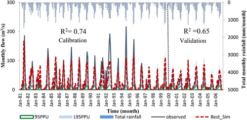
Table 6. SWAT hydrological model performance under validation and calibration periods of observed streamflow in Mojo catchment.

Parameter	Calibration	Validation
Nash-Sutcliffe efficiency (ENS)	0.73	0.61
Coefficient of determination (R^2)	0.74	0.65
Percent bias (PBIAS)	1.6	0.7
P-factor	0.56	0.31
R-factor	0.44	0.40

Setegn et al. (2011), Santhi et al. (2001), Moriasi et al. (2007), and Benaman et al. (2005) suggested that the prediction efficiency of the calibrated model can be a good agreement if R² and NES values are greater than 0.6 and when the value of PBIAS is between ±15 ≤ and ≤ ±30. In this study, the values of R² and NSE were 0.74 and 0.65, respectively, which shows good relation with (Abbaspour et al. 2007a), and the PBIAS which is 1.65 and 0.7 for calibration and validation then the result is more performed according to Gupta et al. (1999) of the observed and the simulated streamflow of the Mojo catchment showed good relations with reasonable performance (Gonfa and Kumar, 2016).

4.3. Performance evaluation of climate GCM models

Analyzing the performances of GCM models with the SWAT model shows a good agreement in Ethiopia basins for instance (Setegn et al. 2011; Dile et al. 2013; Jilo et al. 2019). Each scholar concludes that the SWAT model with an integration of climate scenario data shows remarkable performance. For instance, Jilo et al. (2019) show that calibration and validation for streamflow simulation obtained satisfactory results of fit with R² of 0.8 and 0.77 and NSE coefficients of 0.73 and 0.63 within the lower Awash basin. So, the SWAT model shows good performance of PBIAS, R^2, and NES in this watershed.

4.3.1. Validation of GCMs models

After the Calibration of the 19-year data streamflow validation was conducted based on a 5-year simulation from 2001 to 2005. Table 7 indicates four GCM’s used to select for the comparison of a better-performed Model without Bias correction over Mojo Watershed. Applying the SWAT model has been frequently used to investigate climate change impacts on agro-hydrological systems (Emami and Koch 2018). So, SWAT validates the observed data and every four candidates’ GCMs and the simulated result shows a good argument with climate models which is related (Jilo et al. 2019). So, to analyze, the performance of the candidate models in the catchment historical data was used. The validation statistics for the observed and candidate models are shown in Tables 7 and 8.

Table 7. SWAT hydrological model performance under validation and calibration periods of GCM models and observed data.

Parameter	Calibration		Validation
	Observed	MIROC-MIROC5	IPSL-IPSL-CM5A-MR	MPI-M-MPI-ESM-LR	CCma-CanESM2
(NES)	0.73	0.13	0.02	0.16	0.16
(R^2)	0.74	0.17	0.01	0.21	0.29
(PBIAS)	1.6	65.7	70.8	42.3	93.5

Table 8. Selected GCM models used for analysis.

Id No	Model
1	MIROC-MIROC5
2	MPI-M-MPI-ESM-LR

Teutschbein and Seibert (2012) indicate that Models that performed with the least Percent of Bias indicated good underlying atmospheric dynamics. From those candidates’ validated models, two models were highlighted for bias correction as having reasonable skills in the Mojo watershed, Max Planck Institute for Meteorology Earth System Model (MPI-M-MPI-ESM-LR), and the Model for Interdisciplinary Research on Climate (MIROC-MIROC5).

4.3.2. Analysis of bias corrected climate data and observed data

Analysis of the bias correction is more important before proceeding to the next level to decrease the systematic statistical deviation of climate input data from the observational data (Zhou et al. 2014; Tong et al. 2017; Guo et al. 2018). One way of bias correction is to construct a transfer function (TF) to match the cumulative distribution functions (CDF) of modeled and observed data from large-scale climatic variables. Models bias correction was examined based on a historical period (1981–2005), observed data (1981–2005), and future scenario data (RCP4.5 and RCP8.5) from 2006 to 2080 were corrected. The correction was conducted for daily precipitation (PCP), temperature maximum (Tmax), and minimum (Tmin), for the candidate models and performs good relations with the observed precipitation and temperature data as shown in Figure 5.

Figure 5. Shows the Cumulative Distribution Function before and after bias correction for observed data and Historical data from (1981-2005), fig (A) and (B) Gamma distribution for precipitation of GCMs model MPI-M-MPI-ESM-LR and MIROC-MIROC5, respectively, normal distribution (C, D), for temperature min, (E and F) for temperature max.

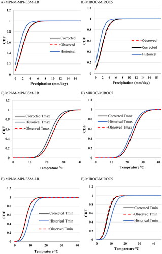
SWAT well simulates the hydrology of the Mojo catchment and is forced to generate historical streamflow as well as future scenario streamflow under both bias-corrected precipitation and temperature climate data to analyze the performance. Models that performed with the least Percent of Bias indicated good underlying atmospheric dynamics (Teutschbein and Seibert2012). From the validation, two models were highlighted for bias correction as having reasonable skill in the region. Table 9 shows the relationship between bias-corrected streamflow output and observed streamflow for the selected GCMs models and, the performance of PBIAS was increased for both models.

Table 9. Performance evaluation streamflow validation output of model MIROC-MIROC5 and MPI-M-MPI-ESM-LR.

Parameter	Calibration	Validation
	Observed	MIROC-MIROC5	MPI-M-MPI-ESM-LR
(NES)	0.73	0.43	0.53
(R^2)	0.74	0.47	0.54
(PBIAS)	1.6	9.6	5.1

4.4. Analysis of climate change future scenarios

Analysis of the future scenario was done for two selected GCMs models. The analysis is classified into three categories from 2006 to 2030 Near future, from 2031 to 2055 mid future, and from 2056 to 2080 far future. Calibration and validation were done in Section 4.2 after fitting the sensitive parameters.

4.4.1. Change in projected precipitation GCM scenarios

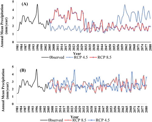
The result of the study after bias corrections of raw precipitation shows that the mean annual precipitation in the future selected models generally shows fluctuation over the Mojo catchment. It seems that the change occur in the Awash basin also Taye (2018) and Hailemariam (1999) used old SERES. The change in precipitation for both model scenarios shows slightly different behavior in the model scenarios and periods. Concerning the baseline period, Figure 6 shows that the change in mean annual precipitations varies over MIROC-MIROC5 model scenarios showing an increasing change from +17 to +35% for the entire period under RCP4.5 and a decreasing change has shown under RCP8.5 climate scenarios over all future periods from 34.86 to 18.78%. Also, model MPI-M-MPI-ESM-LR shows a slight decrease in RCP 4.5 ranging from 25.41 to 24.52% and an increased show under RCP 8.5 varies from 23.68 to 25.85% for all scenarios. Findings that support this output, Intergovernmental Panel on Climate Change IPCC (2014) reported an increase in precipitation with heavy precipitation events over the world.

Figure 6. Annual precipitation (1981–2080) at Mojo catchment for a model, (A) MIROC-MIROC5,(B) MPI-M-MPI-ESM-LR under RCP 4.5 and RCP 8.5 climate scenario.

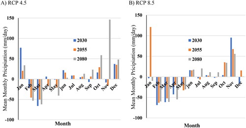
In all future periods, Model MPI-M-MPI-ESM-LR shows that Kiremt (wet) season (June–September) means monthly precipitation change shows a cumulative increasing change over both scenarios. Under RCP 4.5 the trend changes from 27% in the Near period (2030) to 37.4% at Mid and 39.3% under the Far Future period (Figure 7). But the trend under RCP 8.5 shows less increment compared to RCP 4.5 which is 14.3% in the Near, 10.8 % in Mid periods, and 60.1 % in the Far Future period. Belg (short rainy) season (February–May) is knowns as the growing season which is expected to be produced in Ethiopia. The change in precipitation in this season shows a major decline in both RCPs by −81.5% in the Near period, −133.2% in Mid Future, and −179.7 % in the Far future period under RCP 4.5 and also under RCP 8.5 the change decreases by −106.5% at Near, −133.2% at Mid and −206.2 % at a Far future period. This trend shows that the entire season going to be dry. Apart from that the Bega (dry) season (October–January) showed an increasing trend of 122% at Near and 69.4% at Mid Period and 286.9% at Far Future period under RCP4.5 and 49.6% at Near,239.6% at Mid and 81.1% at Far Future period.

Figure 7. Annual monthly mean of precipitation (2006–2080) for the Model MPI-M MPI-ESM-LR under RCP 4.5 and 8.5.

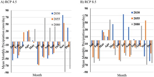
The Cumulative change in precipitation trend over the model MIROC-MIROC5 shows that in the rainy season Kiremt (wet) season (June–September) expects less precipitation in both RCPs. In this season under RCP 4.5, a change in precipitation shows a decreasing trend of −195.2% at Near and −188.7 at Mid period, But in the Far Future period the trend increases by 139.4% (Figure 8). Under RCP 8.5 the change in precipitation increases by 129.3 % in the Near period but the Mid and Far Future period decreases by −158% and −167.4%, respectively. Bega (dry) season (October–January) shows variety in a change for both RCPs by an increase of 51.3% at Near Period, and decrease by −8.1% at Mid, −200.9% at Far Future under RCP4.5 and also under RCP 8.5 the change increase by 129.3% at Near Period, and decrease by −158% at Mid and −167.4% at Far Future period. The Belg (short rainy) season (February–May) shows a different trend under RCP 4.5 this change decrease by −28.4% in the Near and increases by 16.1% in the Mid and 19% in Far Future Period (Figure 8). The results of increased precipitation were related to other findings reported over the Awash basin (Taye 2018). Also, under RCP 8.5 the trend shows an increased chance of 66.4 % in the Near Period and decreases by −23% in the Mid and −28.7 in Far Future Period.

Figure 8. Annual monthly mean of precipitation (2006–2080) for the Model MIROC-MIROC5 under RCP 4.5 and 8.5.

4.4.2. Change in projected temperature GCM scenarios

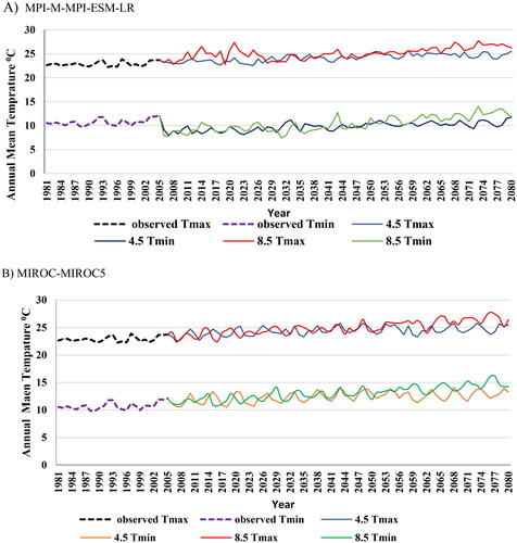
After bias correction, Mojo catchment exhibits an increase in projected minimum and maximum temperature under both GCM models and RCP climate scenarios (Figure 9). The model MIROC-MIROC5 mean annual minimum temperature increases from +1.19$°\mathrm{C}$ to + 3.57$°\mathrm{C}$ under RCP 8.5 and from + 1$°\mathrm{C}$ to + 1.99$°\mathrm{C}$ under RCP 4.5 such analysis is visible with the result (Fox et al. 2018). Similarly, the mean annual maximum temperature showed an increasing trend and varies from + 1$°\mathrm{C}$ to + 1.74$°\mathrm{C}$ under RCP8.5 and from + 0.99$°\mathrm{C}$ to + 1.74$°\mathrm{C}$ under RCP4.5 in the future periods. For the MPI-M-MPI-ESM-LR model, the maximum temperature in both scenarios is becoming to increase from + 0.45$°\mathrm{C}$ to 1.875$°\mathrm{C}$ under RCP 4.5 and +0.47$°\mathrm{C}$ to 1.97$°\mathrm{C}$ under RCP 8.5, and the minimum temperature shows a decreasing variation from −1.81$°\mathrm{C}$ to −0.30$°\mathrm{C}$ under RCP 4.5 for all periods and from −1.55$°\mathrm{C}$ to −0.83$°\mathrm{C}$ for RCP 8.5 till Mid period but in the Far future period, it is becoming to increase by 1.21$°\mathrm{C}.$

Figure 9. Annual monthly mean of temperature maximum and minimum (1981–2080) at Mojo catchment for model MPI-M-MPI-ESM-LR (A) and MIROC-MIROC5 (B) under RCP4.5 and RCP8.5 climate scenario.

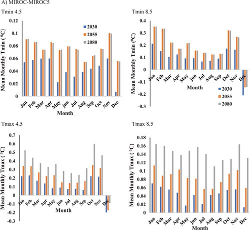
The seasonal variation of change in temperature over the Mojo catchment shows that reasonable change in both GCM models. Model MIROC-MIROC5 shows that the maximum temperature in the Kiremt season (June–September) increases in both RCPs by 0.15$°\mathrm{C}$ at Near to 0.27$°C$ at Mid and Far Future Period under RCP 4.5. Under RCP 8.5 the trend shows the same increment as RCP 4.5 but the change differs in the Far future period by 0.54$°\mathrm{C}.$ The minimum temperature also increases in both RCPs by 0.32$°\mathrm{C}$ in Near Period to 0.55$°\mathrm{C}$ at the Mid and Far future period under RCP 4.5 and the trend changes under RCP 8.5 from 0.3$°\mathrm{C}$ at Near to 0.61$°\mathrm{C}$ and 1.11$°C.$ During the Belg season (February–May), the maximum temperature still shows an increasing change in both RCP by 0.17 $°\mathrm{C}$ at Near to 0.33$°\mathrm{C}$ at Mid and Far Future Period under RCP 4.5 and under RCP 8.5 the temperature increases by 0.19$°\mathrm{C}$ at Near to 0.36$°\mathrm{C}$ at Mid and 0.58 $°C$ at Far Future Period. Similarly, the minimum temperature under the Belg season shows an increasing change in both scenarios by 0.33$°\mathrm{C}$ at Near, 0.8$°\mathrm{C}$ at Mid, and 0.79$°\mathrm{C}$ Far Future Period under RCP 4.5 and under RCP 8.5 the temperature increases by 0.46$°\mathrm{C}$ at Near, 0.84$°\mathrm{C}$ at Mid and 1.5$°\mathrm{C}$ at Far Future Period. The Bega (dry) season (October–January) shows the mixed change in maximum and minimum temperature under both scenarios. In this season the minimum temperature shows an increasing change of 0.46$°\mathrm{C}$ in the Near and 0.93$°\mathrm{C}$ Mid Future Period and 0.95$°C$ in the Far Future Period under RCP 4.5 and under RCP 8.5 the change increased by 0.62$°\mathrm{C}$ at Near, 1.06$°\mathrm{C}$ at Mid and 1.54$°\mathrm{C}$ at Far Future Period. The maximum temperature shows an increasing change from 0.22$°\mathrm{C}$ at Near, 0.32$°\mathrm{C}$ Mid, and 0.31$°\mathrm{C}$ at Far Future Period under RCP 4.5 and under RCP 8.5 the increased trend shows from 0.19$°\mathrm{C}$ at Near, 0.36$°\mathrm{C}$ at Mid and 0.6$°\mathrm{C}$ Far future period. In this season the month of December shows a decreasing trend in temperature in both scenarios (Figure 10).

Figure 10. Annual Monthly mean of temperature maximum and minimum (2006–2080) for the Model MIROC-MIROC5 under RCP 4.5 and 8.5.

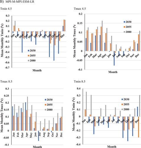
Under the model MPI-M-MPI-ESM-LR, the seasonal variation of temperature change shows a much more decrease in both scenarios. The maximum temperature variation over the Kiremt season shows a decreasing trend by −0.14$°\mathrm{C}$ at Near Period and increases by 0.4$°\mathrm{C}$ at Mid to 0.15$°\mathrm{C}$ at Far Future Period under RCP 4.5 and under RCP 8.5 the change decreases by −0.03$°C$ at Near Period and increases by 0.1$°C$ at Mid and 0.35 at Far Future period. On the other hand, the minimum temperature shows a decreasing change from −0.98$°C$ at Near, −0.39$°\mathrm{C}$ at Mid, and −0.21$°\mathrm{C}$ at Far Future Period under RCP 4.5 and RCP 8.5 also decreases by −0.63$°\mathrm{C}$ at Near and −0.28$°\mathrm{C}$ at Mid Future period and increases by 0.16$°C$ at Far Future Period. Belg season shows an increasing maximum temperature change in both RCPs by 0.12$°C$ at Near, 0.28$°\mathrm{C}$ at Mid, and 0.31$°\mathrm{C}$ at Far Future Period under RCP 4.5 and Under RCP 8.5 the change also increases by 0.3$°\mathrm{C}$ at Near, 0.29$°\mathrm{C}$ at Mid and 0.58$°\mathrm{C}$ at Far Future Period. Unlike form maximum temperature the change in minimum temperature shows a decreasing trend by −0.93$°\mathrm{C}$ at Near, −0.11$°\mathrm{C}$ at Mid Future Period, and increase by 0.13 at Far Future Period under RCP 4.5 and under RCP 8.5 the change also decreases by −0.49$°\mathrm{C}$ at Near, −0.56$°\mathrm{C}$ at Mid Future Period and increases by 0.81$°\mathrm{C}$ at Far Future Period. In Bega season shows a decrease in change under both minimum temperatures of RCPs by −0.83$°\mathrm{C}$ at Near, −0.2$°\mathrm{C}$ at Mid Period, and −0.17$°\mathrm{C}$ at Far Future Period under RCP 4.5 and RCP 8.5 also shows decreases in trend by −0.59$°\mathrm{C}$ at Near, −0.14 at Mid and increase change at Far Future by 0.59$°\mathrm{C}.$ The maximum temperature increases in both RCPs by 0.25$°\mathrm{C}$ at Near, 0.44$°\mathrm{C}$ at Mid, and 0.51$°\mathrm{C}$ at Far Future Period under RCP 4.5 and RCP 8.5 the change also increased by 0.59 at Near, 0.5 at Mid, and 0.8 at Far Future Period. Taye (2018) also shows the seasonal variation of the average temperature change factors for the entire Awash basin for both maximum and minimum temperature near-term to the end of the century the increase in temperature becomes high for both maximum and minimum temperatures (Figure 11).

Figure 11. Annual Monthly mean of Temperature maximum and minimum change (2006–2080) for the Model MPI-M-MPI-ESM-LR under RCP 4.5 and 8.5.

4.5. Hydrological change of projected precipitation and temperature on streamflow

4.5.1. Change in projected streamflow

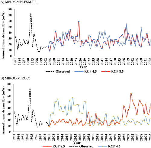
SWAT hydrological model calibrated and validated the streamflow of Mojo catchment at gauged station and model results of streamflow were considered for comparative analysis with a baseline period from 1981–2005 and projection periods at 2030 (2005–2030), 2055s (2031–2055), and 2080s (2056–2080) under both GCMs models and climate scenarios. Figure 12 shows the annual mean flow of two models relative to the baseline (observed). The model MPI-M-MPI-ESM-LR shows that the baseline streamflow for both scenarios increases relative to the baseline. Under RCP 4.5 the stream increases by 4.62 m³/s, 4.30 m³/s, and 7.79 m³/s by the year Near (2030), Mid (2055), and Far (2080), respectively. For RCP 8.5 it increases by 6.68 m³/s, 2.64 m³/s, and 6.31 m³/s by the year Near, Far, and Future periods, respectively. Findings related to Gizaw et al. (2017) also show an increase in the projected annual streamflow in the Awash basin by the 2050s and 2080s. Change in model MIROC-MIROC5 shows a decreasing streamflow change at the Near and Mid period of RCP 4.5 scenario by −6.32 m³/s and −5.08 m³/s, respectively. Some of the results Daba (2015) and Taye (2018) which is related to decreasing streamflow happened in 2050 and 2080 over the Awash basin but unlike the Mojo catchment the decrease starts in the Near and Mid periods under RCP 4.5, But in Far future period, the streamflow shows increases change by 19 m³/s. Similarly, the RCP 8.5 Near period increases by 18.33 m³/s, 4.27 m³/s at Mid, and decreases by 5.76 m³/s in the Far future period which is the same as those (Taye 2018) and (Daba 2015) (Figure 12).

Figure 12. The annual mean of simulated streamflow (1981–2080) at Mojo catchment for model MPI-M-MPI-ESM-LR (A) and MIROC-MIROC5 (B) under RCP4.5 and RCP8.5 climate scenarios.

Seasonal projection streamflow showed a mixed increasing and decreasing trend in both Models (Figure 13) This variation of Streamflow under the model MPI-M-MPI-ESM-LR show at Kiremt (main rainy) season (June–September) the streamflow increases in both RCPs except September at Near and Mid period for both RCPs. Also, Bega (dry) season (October–January), the trend shows an increase in change in October and January and a decreasing trend in November and December under RCP 4.5 and RCP 8.5.

Figure 13. The annual mean of simulated streamflow change (%) (1981-2080) at Mojo catchment for model MPI-M-MPI-ESM-LR and MIROC-MIROC5 under RCP4.5 and RCP8.5 climate scenarios.

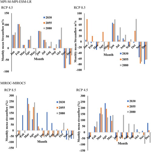
Similarly, under RCP 4.5 the Belg season (February–May), streamflow shows increased change in all periods except March at Far future and May for all periods. On the reverse RCP 8.5 shows decreasing in change for all periods except February and April in Mid future period.

The seasonal variation continues under the model MIROC-MIROC5 showing that at the Kiremt season the trend decreased in both RCPs except June, July, August, and September at a Far period under 4.5 and the Near period under 8.5 scenarios. For the short rainy season, Belg periods RCPs an increasing change shows in both RCPs for entire periods except February at the Far future period under RCP 8.5.

Bega season shows a decrease in the change in both RCPs except October and December in the Near and Mid Future period and November in the Near Future period under RCP 4.5. Under RCP 8.5 October and November in Mid future period and October in the far-future period show increasing in change see Figure 13.

4.5.2. Impact of future precipitation and temperature change on the streamflow

The variation of increasing and decreasing precipitation as well as temperature projection that leads to fluctuation over the streamflow of Ethiopia basins Mengistu and Sorteberg (2012), Gizaw et al. (2017) and Chaemiso et al. (2016) this variation has also been shown in the Mojo catchment.

The models used in the analysis show that the variation of streamflow occurs with the different occurrences of temperature and precipitation results. The model MPI-M-MPI-ESM-LR shows that the annual mean of stream flow under RCP 8.5 indicates that increase of 29.7 m³/s at Near (2006-2030), 25.0 m³/s at Mid (2031-2055) and 28.7 m³/s at Far period. Also, the precipitation increased by 2.35 mm/day, 2.45 mm/day, and 2.57 mm/day under the Near, Mid, and Far periods, respectively, So this variation has relation to the stream flow of Mojo catchment with increased precipitation leads to increase streamflow which related with Jilo et al. (2019) over logiya catchment. Under RCP 4.5 the maximum temperature shows 24.55 °C in the Near, 24.60 °C in Mid periods, and 26.22 °C under the Far period, and the minimum temperature shows 9.17 °C, 9.90 °C, and 11.95 °C under a period of Near, Mid and Far, respectively. Similarly, under the RCP 4.5, the streamflow variation shows a decrease in trend from 29.12 m³/s in the Near, 27.06 m³/s Mid future, and 29.18 m³/s in the Far Future periods. and the maximum temperature becomes increases from 23.35 °C to 25.05 °C under the Near and Mid period the decrease in temperature occurred under the Far period by 24.77 °C leads to decreasing in streamflow in the Near and Mid period which is related to (Dile et al. 2013).

The variation under the model MIROC-MIROC5 shows that the annual mean streamflow decrease trend under RCP 8.5 with an increase of maximum temperature from 40.78 m³/s to 18.16 m³/s under Near and Mid period and 16.68 m³/s under Far future period and the temperature from 23.90 °C to 24.82 °C under the period of Near and Mid period and 26.18 °C in the period of Far future. The condition becomes more favorable to high evapotranspiration and causes decreased streamflow by the increase in maximum temperature in both periods of Near and Mid Future as well as Far future of RCP 8.5 which is a related result with Taye (2018) at Awash basin and Molla and Abdisa (2018) at Baro Akobo basin. Increases streamflow under RCP 4.5 from 16.12 m³/s to 17.55 m³/s in the period of Near and Mid Future and 41.74 m³/s in the period of the Far Future.

Under RCP 8.5 and decrease of precipitation from 3.29 mm/day to 1.82 mm/day by the period of Near and Mid future and 1.77 mm/day under the Far future period. The minimum temperature in both scenarios shows an increasing trend under RCP 8.5 from 11.93 °C to 12.91 °C under the Near and Mid period and also 14.70 °C under the far period. For the RCP 4.5, the minimum temperature shows 11.14 °C, 12.71 °C, and 12.70 °C under the Near, Mid, and far future periods, respectively.

5. Conclusions

The climate change effect is likely to be alterations in hydrologic cycles and changes in water availability.

The study has shown that climate change has major implications for the hydrological response in the Mojo watershed. Analysis of the impact of climate change on Mojo catchment hydrology is using data resulting from CORDEX-Africa mid-range and high-level RCP climate scenarios (RCP 4.5 and RCP 8.5). These ranges give additional input options for the poly makers and water resource planners especially for estimating hydrological scenarios. Projected precipitation and temperature from ensemble CORDEX-Africa RCP scenarios have systematic errors (bias) that may lead to biased simulated streamflow which is not corrected by calibration of the hydrological model. However, Quantile mapping with Gamma distribution for precipitation and Normal distribution method for temperature was used to correct the biases and improve precipitation and streamflow simulations.

The analysis has been done in three periods Near future (2006-2030), Mid future (2031-2055), and Far future (2056-2080) periods under Mid-range RCP 4.5 and high-level RCP 8.5 climate scenarios. Overall, Under RCP8.5 and RCP4.5, the average projected temperature consistently increases by 0.76 °C and 0.75 °C, respectively, across the Mojo catchment and decreases average precipitation projection by 16% under RCP8.5 and increases by 18% under RCP 4.5 in the model of MIROC-MIROC5 due to such visual variation the streamflow shows a decrease under RCP 8.5 and RCP 4.5 by 8.3 m³/s and 1.27 m³/s, respectively, which is the direct impact on the watershed. On the other hand, Under the model, MPI-M-MPI-ESM-LR the projected precipitation shows a slight decrease in the RCP 4.5 by 0.85% and a 2.17% increase rate in the RCP 8.5 scenario and Under RCP 4.5 and RCP 8.5, the Average temperature shows 1.425 °C and 1.5 °C increasing rate, respectively, but, the stream flow shows increasing rate by 3.17 m³/s and 0.37 m³/s under RCP 4.5 and RCP 8.5, respectively. So, the result shows that the variation of temperature and precipitation has a direct impact on the stream flow of the catchment it will also cause high floods in the future.

The findings in this study revealed that models of MPI-M-MPI-ESM-LR and MIROC-MIROC5 have the best agreement with the ground observational data of Mojo catchment after selecting the performed GCM models two of them show good relation with the observed data which are (R² = 0.54, NES = 0.53) and (R² = 0.47, NES = 0.43) over the Mojo catchment, respectively. The performance assessment of climate GCMs models over the Mojo catchment reviles that R² = 0.74, NES = 0.73 shows a good relationship with the observed data. So, the SWAT model is so much more suitable for the catchment of the study area.

The seasonal variation of Kiremt and Bega including Belg season shows a mixed trend. Projected higher temperature and precipitation increases under RCP4.5 and RCP8.5 climate scenarios are expected to decrease the projected streamflow of the Mojo catchment. The seasonal variation results in the Near, Mid, and Far period is good inputs for climate change and will have implications in changing the frequency of extreme events. This study result showed that climate change will affect the planning and operation of the Mojo catchment. Therefore, the effect of projected precipitation and streamflow should be included in the feasibility assessment of Mojo catchment planning. Future research on impact assessments should focus on integrated approaches linking climate, hydrology, water resources, and ecosystem models to sustain and improve the development of the river and its basin in a changing environment. As this study considers land use and soil data to remain constant in the future period, we recommend other researchers forecast land use for the future period.

Authors’ contributions

The authors Mikhael G. Alemu, Melsew A. Wubneh, and Tadege A. Worku, conceived the presented idea. The corresponding author Melsew Amsalu developed the theory and performed the computations. Other authors have reviewed the work and made an edition.

Acknowledgments

We gratefully acknowledge all offices and personalities who have given data for our study. Ministry of Water Irrigation and Energy, Oromia Region Meteorological Agency, and Awash Basin authority are government agencies all the necessary data has been collected.

Disclosure statement

We (authors) have to declare that we have no known personal relationships that could have appeared to influence the work reported in this paper.

References

- Abbaspour KC, Yang J, Maximov I, Siber R, Bogner K, Mieleitner J, Zobrist J, Srinivasan R. 2007a. Modelling hydrology and water quality in the pre-alpine/alpine Thur watershed using SWAT. J Hydrol. 333(2-4):413–430.
- Abbaspour KC, Yang J, Maximov I, Siber R, Bogner K, Mieleitner J, Zobrist J, Srinivasan R. 2007b. SWAT-CUP Calibration and Uncertainty Programs for SWAT. In MODSIM 2007 international congress on modelling and simulation, modelling and simulation society of Australia and New Zealand. Dübendorf, Switzerland: Swiss Federal Institute of Aquatic Science and Technology; p. 1596–1602.
- Abraham LZ, Roehrig J, Chekol DA. 2007. Climate change impact on Lake Ziway watershed water availability, Ethiopia. Institute for Technology in the topics, University of Applied Science: Cologne, Germany.
- Adeba D, Kansal ML, Sen S. 2016. Economic evaluation of the proposed alternatives of inter-basin water transfer from the Baro Akobo to Awash basin in Ethiopia. Sustain Water Resour Manag. 2(3):313–330.
- Alemseged TH, Tom R. 2015. Evaluation of regional climate model simulations of rainfall over the Upper Blue Nile basin. Atmos Res. 161–162:57–64.
- Arnold JG, Moriasi DN, Gassman PW, Abbaspour KC, White MJ, Srinivasan R, Santhi C, Harmel D, Jha MK. 2012. SWAT: model use, calibration, and validation. Trans ASABE. 55(4):1491–1508.
- Bekele D, Alamirew T, Kebede A, Zeleke G, Melesse AM. 2019. Modeling climate change impact on the hydrology of Keleta watershed in the Awash River basin, Ethiopia. Environ. Model. Assess. 24(1):95–107.,
- Benaman J, Shoemaker CA, Haith DA. 2005. Calibration and validation of soil and water assessment tool on an agricultural watershed in upstate New York. J Hydrol Eng. 10(5):363–374.
- Bhatta B, Shrestha S, Shrestha PK, Talchabhadel R. 2019. Evaluation and application of a SWAT model to assess the climate change impact on the hydrology of the Himalayan river basin. Catena. 181:104082.
- Chaemiso SE, Abebe A, Pingale SM. 2016. Assessment of the impact of climate change on surface hydrological processes using SWAT: a case study of Omo-Gibe river basin, Ethiopia. Model Earth Syst Environ. 2(4):1–15.
- Cheung WH, Senay GB, Singh A. 2008. Trends and spatial distribution of annual and seasonal rainfall in Ethiopia. Int J Climatol. 28(13):1723–1734.
- Choi J, Socolofsky SA, Olivera F. 2008. Hourly disaggregation of daily rainfall in Texas using measured hourly precipitation at other locations. J Hydrol Eng. 13(6):476–487.
- Christensen JH, Christensen, OB. 2007. A summary of the PRUDENCE model projections of changes in European climate by the end of this century. Climatic Change. 81(S1):7–30.
- Conway D. 1997. A water balance model of the upper Blue Nile in Ethiopia. Hydrological Sciences J. 42(2):265–286.
- Cooper, P. J., Dimes, J., Rao, K. P. C., Shapiro, B., Shiferaw, B., & Twomlow, S. (2008). Coping better with current climatic variability in the rain-fed farming systems of sub-Saharan Africa: an essential first step in adapting to future climate change? Agriculture, Ecosystems & Environment, 126(1-2), 24–35.
- Daba M. 2015. Evaluating potential impacts of climate change on surface water resource availability of upper Awash sub-basin, Ethiopia rift valley basin.
- Dile YT, Berndtsson R, Setegn SG. 2013. Hydrological response to climate change for Gilgel Abay River, in the Lake Tana Basin – Upper Blue Nile basin of Ethiopia. ed. Juan A. Añel. PLoS ONE. 8(10):e79296. https://doi.org/10.1371/journal.pone.0079296.
- Dodman D. 2009. Blaming cities for climate change? An analysis of urban greenhouse gas emissions inventories. Environ Urban. 21(1):185–201.
- Emami F, Koch M. 2018. Sustainability assessment of the water management system for the Boukan Dam, Iran, using CORDEX-South Asia climate projections. Water (Switzerland). 10(12):1–21.
- Emiru NC, Recha JW, Thompson JR, Belay A, Aynekulu E, Manyevere A, Demissie TD, Osano PM, Hussein J, Molla MB, et al. 2021. Impact of climate change on the hydrology of the upper Awash river basin, Ethiopia. Hydrology. 9(1):3.
- Eshetu M. 2020. Hydro-climatic variability and trend analysis of Modjo river watershed, Awash river basin of Ethiopia. Hydrol Curr Res. 11(2):1–8.
- Fox KM, Nelson S, Frankenberger TR, Langworthy M. 2018. Climate change adaptation in Ethiopia: developing a method to assess program options. In Resilience. Elsevier; p. 253-265.
- Getahun YS, van Lanen IH, Torfs PP. 2014. Impact of climate change on hydrology of the upper Awash river basin (Ethiopia): inter-comparison of old SRES and new RCP Scenarios (Doctoral dissertation, Wageningen University).
- Girma W. 2013. Hydrological impacts of climate change in lake Hawasa watershed Ethiopia [MSc thesis].
- Gizaw MS, Biftu GF, Gan TY, Moges SA, Koivusalo H. 2017. Potential impact of climate change on streamflow of major Ethiopian rivers. Clim Change. 143(3–4):371–383.
- Gonfa ZB, Kumar D. 2015. Optimal land use planning in Mojo watershed with multi-objective linear programming. Am Int J Res Humanit Arts Soc Sci. 13(1):10–17.
- Gonfa ZB, Kumar D. 2016. Application of soil and water assessment tool model to estimate runoff and sediment yield from Mojo watershed. Int J Innov Res Sci Eng Technol. 5(2):2081–2091.
- Gudeta K, Argaw M, Kindu M. 2022. Identifying priority Areas for Conservation in Mojo River Watershed of Ethiopia Using GIS-based Erosion Risk Evaluation. In state of the Art in Ethiopian Church forests and Restoration Options. Springer, cham; p. 267-285.
- Guo L-Y, Gao Q, Jiang Z-H, Li L. 2018. Bias correction and projection of surface air temperature in LMDZ multiple simulation over central and eastern China. Adv Clim Change Res. 9(1):81–92.
- Gupta HV, Sorooshian S, Yapo PO. 1999. Status of automatic calibration for hydrologic models: comparison with multilevel expert calibration. J Hydrol Eng. 4(2):135–143.
- Hailemariam K. 1999. Impact of climate change on the water resources of Awash river basin, Ethiopia. Clim Res. 12(2–3):91–96.
- Heo JH, Ahn H, Shin JY, Kjeldsen TR, Jeong C. 2019. Probability distributions for a quantile mapping technique for a bias correction of precipitation data: a case study to precipitation data under climate change. Water. 11(7):1475.
- IPCC. 2014. Mitigation of climate change. Contribution of Working Group III to the Fifth Assessment Report of the Intergovernmental Panel on Climate Change 1454.
- Jaramillo J, Muchugu E, Vega FE, Davis A, Borgemeister C, Chabi-Olaye A. 2011. Some like it hot: the influence and implications of climate change on coffee berry borer (Hypothenemus hampei) and coffee production in East Africa. PLoS One. 6(9):e24528.
- Jilo NB, Gebremariam B, Harka AE, Woldemariam GW, Behulu F. 2019. Evaluation of the impacts of climate change on sediment yield from the Logiya Watershed, Lower Awash Basin, Ethiopia. Hydrology. 6(3):81.
- Mandal U, Sena DR, Dhar A, Panda SN, Adhikary PP, Mishra PK. 2021. Assessment of climate change and its impact on hydrological regimes and biomass yield of a tropical river basin. Ecol Indic. 126:107646.
- Mengistu DT, Sorteberg A. 2012. Sensitivity of SWAT simulated streamflow to climatic changes within the eastern Nile river basin. Hydrol Earth Syst Sci. 16(2):391–407.
- Shimelash M, Tolera A, Tamene A. 2018. Investigating climate change impact on stream flow of Baro-Akobo River Basin. Case study of Baro Catchment. Global Sci J. 6:180–216.
- Moriasi DN, Arnold JG, Van Liew MW, Bingner RL, Harmel RD, Veith TL. 2007. Model evaluation guidelines for systematic quantification of accuracy in watershed simulations. Trans ASABE. 50(3):885–900.
- Moss RH, Edmonds JA, Hibbard KA, Manning MR, Rose SK, van Vuuren DP, Carter TR, Emori S, Kainuma M, Kram T, et al. 2010. The next generation of scenarios for climate change research and assessment. Nature. 463(7282):747–756.
- Nash JE, Sutcliffe JV. 1970. River flow forecasting through conceptual models part I—a discussion of principles. J Hydrol. 10(3):282–290.
- Ongoma V, Chen H, Gao C. 2019. Evaluation of CMIP5 twentieth century rainfall simulation over the equatorial east Africa. Theor Appl Climatol. 135(3-4):893–910.
- Papadimitriou V. 2004. Prospective primary teachers’ understanding of climate change, greenhouse effect, and ozone layer depletion. J Sci Educ Technol. 13(2):299–307.
- Rahmato D. 1999. Water resource development in Ethiopia: issues of sustainability and participation. In Forum for Social Studies.
- Saade J, Atieh M, Ghanimeh S, Golmohammadi G. 2021. Modeling impact of climate change on surface water availability using SWAT model in a semi-arid basin: case of El Kalb River, Lebanon. Hydrology. 8(3):134.
- Santhi C, Arnold JG, Williams JR, Dugas WA, Srinivasan R, Hauck LM. 2001. Validation of the SWAT model on a large river basin with point and nonpoint sources 1. J Am Water Resources Assoc. 37(5):1169–1188.
- Seo S, Kim Y-O. 2018. Impact of spatial aggregation level of climate indicators on a national-level selection for representative climate change scenarios. Sustainability.10(7):2409.
- Setegn SG, Rayner D, Melesse AM, Dargahi B, Srinivasan R. 2011. Impact of climate change on the hydroclimatology of Lake Tana Basin, Ethiopia. Water Resource Res. 47(4).
- Taye M, Dyer E, Hirpa F, Charles K. 2018. Climate change impact on water resources in the Awash basin, Ethiopia. Water (Switzerland). 10(11):1560.
- Taye MT, Ntegeka V, Ogiramoi NP, Willems P. 2011. Assessment of climate change impact on hydrological extremes in two source regions of the Nile river basin. Hydrol Earth Syst Sci. 15(1):209–222.
- Teutschbein C, Seibert J. 2012. Bias correction of regional climate model simulations for hydrological climate-change impact studies: review and evaluation of different methods. J Hydrol. 456–457:12–29.
- Thomson AM, Calvin KV, Smith SJ, Kyle GP, Volke A, Patel P, Delgado-Arias S, Bond-Lamberty B, Wise MA, Clarke LE, et al. 2011. RCP4. 5: a pathway for stabilization of radiative forcing by 2100. Clim Change. 109(1-2):77–94.
- Tong Y, Gao XJ, Han ZY, Xu Y. 2017. Bias correction of daily precipitation simulated by RegCM4 model over China. Chin J Atmos Sci. 41(6):1156–1166.
- Winchell M, Srinivasan R, Luzio MD, Arnold J. 2010. Arc SWAT interface for SWAT 2009. Users’ guide. Grassland, Soil and Water Research Laboratory. Agricultural Research Service, and Blackland Research Center. Temple (TX): Texas Agricultural Experiment Station; p. 495.
- Wood AW, Leung LR, Sridhar V, Lettenmaier DP. 2004. Hydrologic implications of dynamical and statistical approaches to downscaling climate model outputs. Clim Change. 62(1-3):189–216.
- Worku G, Teferi E, Bantider A, Dile Y. T, Taye MT. 2018. Evaluation of regional climate models performance in simulating rainfall climatology of Jemma sub-basin, Upper Blue Nile Basin, Ethiopia. Dynamics of Atmosphers and Oceans. 83:53–63.
- Zhou L, Pan J, Zhang L. 2014. Analysis on statistical bias correction of daily precipitation simulated by regional climate model. J Trop Meteorol 30(1).