Integrating multi-criteria analysis and spherical cellular automata approach for modelling global urban land-use change

Abstract

Existing geosimulation land-use change models are predominantly designed to operate at local or regional spatial scales. When these models are applied on data at the global level, they do not consider the effects of spatial distortions caused by the curvature of the Earth’s surface and often lack some refinements related to land suitability analysis. Therefore, the main objective of this study is to integrate multi-criteria evaluation with spherical cellular automata, to develop a novel modelling approach for simulating global urban land-use change. The world region is clustered into sub-regions to improve the suitability analysis. The obtained results reveal differences in urban growth rate and the size of the extent across the four clusters. The 64% of the total global urbanization are occurring in urban region clusters characterized by high gross domestic product and population density, while urban regions in isolated locations have the lowest urban growth rate.

Keywords:

• Global land use change modelling
• geographic automata systems
• spherical cellular automata
• multicriteria evaluation
• geographic information systems

1. Introduction

Land-use and land-cover changes can be perceived as a complex dynamic spatial system that characterizes the alteration of the Earth surface mainly through human activities thus having different consequences on the natural environment (Turner et al. 2021; Winkler et al. 2021). Urban land-use change research studies have become prominent in the past decades due to the several global sustainability problems and consequences associated with urban sprawl (Nuissl and Siedentop 2021). To examine and model urban land-use dynamics, a number of spatially explicit land-use change models reported in the scientific literature were designed mainly for small-scale applications. The utilization of these models for simulating urban land-use change patterns and possible future scenarios at larger spatial scales poses challenges that are peculiar to spatial modelling at the global scale.

Urban land-use models that represent the dynamics of change generally use geospatial data from remote sensing (RS) and geographic information systems (GIS) predominantly in raster GIS data format, thus they are implemented with traditional two-dimensional (2 D) spatial tessellation. While such models are suitable to address dynamics of urban land-use change at the local or regional levels, this however is not suitable when addressing global modelling due to spatial distortions caused by the curvature of the Earth surface. Distortions are minimal at the local level but are however pronounced at larger spatial scales which incur errors in some spatial and statistical analyses, especially at the global level (Hall et al. 2020; Ellis et al. 2021). For example, the shape and size of geospatial data represented in geographic coordinate system (GCS) change from square cells at the equator to triangles at the poles (Zhai et al. 2010; Hojati et al. 2022). Although equal-area projections such as Goode’s Homolosine and Cylindrical equal-area are often used for large-scale spatial analysis, global land-use change models implemented with these projections however produce spatial distortions (Li et al. 2017; Cao et al. 2019). Further, commonly used global equal-area projections still have area and shape distortions when used to represent global raster datasets (de Sousa et al. 2019). Discrete global grid systems (DGGS) have been developed as spatial referencing system which utilizes spherical tessellations to better represent the Earth’s surface (Purss et al. 2019). DGGS provide a geospatial framework for global spatial analyses and modelling with equal surface area cells. DGGS also supports multiple cell typologies including hexagonal grids, which have been receiving considerable interest recently because of the advantages they offer over square and triangle cell types when used for geospatial operations. For instance, hexagonal cells have uniform adjacency and neighbouring relationships and can closely approximate circular regions (Sahr 2011; Zhao et al. 2022). Among regular cells, hexagons are the most compact in tessellating the sphere (Robertson et al. 2020). When used to implement cellular automata (CA) models, hexagonal cells also provide unambiguous spatial neighbourhood and have been indicated to produce more accurate outputs compared to square cells (Iovine et al. 2005; Nugraha et al. 2021). Hexagonal DGGS as a geospatial data model can offer appropriate basis for spatial analysis and simulation at the global level (Kiester and Sahr 2008). Spherical CA also provide a suitable grid topology for modelling and understanding naturally closed systems at the global scale (Ventrella 2011). In a hexagonal grid, the relative location and neighbourhood of cells can be defined using the hexagonal coordinate system which has three coordinate axes that are evenly spaced apart and are usually denoted as $i, j, k.$ A central cell has six neighbouring cells that are equidistant from each other thus making the neighbourhood more compact. Measuring distance on the hexagonal grid can be expressed as the number of cell rings from the origin (Li and Stefanakis 2020).

Existing global urban land-use change modelling approaches simulate urban change using mainly SLEUTH (Zhou et al. 2019), probabilistic (Seto et al. 2012), cellular automata (Li et al. 2016), statistical (Gao and O'Neill 2019), and machine learning techniques (Chen et al. 2022). Although these modelling techniques are capable of representing the determinants of urban land-use change and simulating land-use patterns, the underlying techniques in these models have been criticized for lack of integration of decision-making capabilities (National Research Council 2014; Verburg et al. 2015). Multicriteria evaluation (MCE) techniques have been developed and widely adopted as GIS-based decision-making approaches for solving spatial problems (Malczewski 1996). MCE provides a collection of methods and procedures for structuring and solving decision problems involving multiple criteria and when integrated with GIS can assist in a broad range of spatial and geographical applications (Malczewski and Jankowski 2020). MCE can be utilized in characterizing decision-making processes of various stakeholders and subject experts to solicit their opinions in various stages from choice of criteria to weights. In addition, in land-use change modelling, MCE is often coupled with cellular automata (CA) to enhance the function of transition rules (Wu and Webster 1998; Cao et al. 2014) that improves model capacity to forecast. There has been a significant number of studies that have incorporated MCE methods in CA models of urban land-use change to improve the simulation abilities (Rimal et al. 2018; Mohamed and Worku 2020; Masoudi et al. 2021). However, these studies are conducted at smaller spatial extents with majority of them operationalized at the city or metropolitan region level. Currently, there are no available MCE-CA methods designed to simulate urban development at a global scale.

Given the capabilities of cellular automata to capture local interactions and complexity of space-time dynamics of urban land-use process, the merit of MCE in representing human decision-making for land suitability analysis, and DGGS hexagonal grids in tessellating spherical surfaces, the main objective of this research study is to develop and implement a novel global MCE spherical-CA (MCE-S-CA) model to simulate urban land-use change. The proposed model can be utilized by various stakeholders and interested parties to simulate possible future global-scale urban growth scenarios and examining the causes and effects of urban land-use change on the environment.

2. Methodology

2.1. Datasets

Several geospatial datasets that allow for global Earth coverage have been used in this research study. Due to the unavailability of datasets originally captured in DGGS formats, the study utilized existing geospatial datasets in geographic coordinate system (GCS). Datasets for the years 1995, 2005 and 2015 were used to implement and evaluate the proposed MCE-S-CA model. Global land-use/land-cover data were acquired from the European Space Agency portal (ESA 2017). Gridded population density dataset was obtained from LandScan (Rose et al. 2020) and gross domestic product (GDP) from National Centers for Environmental Information (NCEI) (Ghosh et al. 2011). The location of protected areas was obtained from the World Database on Protected Areas (WDPA) online data catalogue (WDPA 2020). Global digital elevation model (DEM) was acquired from the United States Geological Survey (USGS) data portal (USGS 2020). Also, global road dataset was obtained from the Global Road Inventory Project (Meijer et al. 2018). The proposed modelling framework utilizes data that are mapped to a specified DGGS consisting of hexagonal cells with each covering an area of 0.63 km² with edge and long diagonal dimensions of 0.49 km and 0.99 km, respectively, thus used as the spatial resolution of the model. The conversion of existing spatial datasets to DGG cells follows the techniques described by Robertson et al. (2020).

2.2. Model overview

The systematic workflow of the proposed MCE-S-CA model is presented in Figure 1 and consists of four main steps. The first step entails creating geospatial database and defining the decision problem which in this context involves finding suitable locations for urban development at the global scale and considering the spherical Earth surface. Subsequently, criteria that are relevant to urban development are identified within the urban science literature and corresponding suitability functions are developed for each of them.

Figure 1. Workflow of the MCE-S-CA modelling framework for simulation of the long-term urban growth dynamics at the global scale.

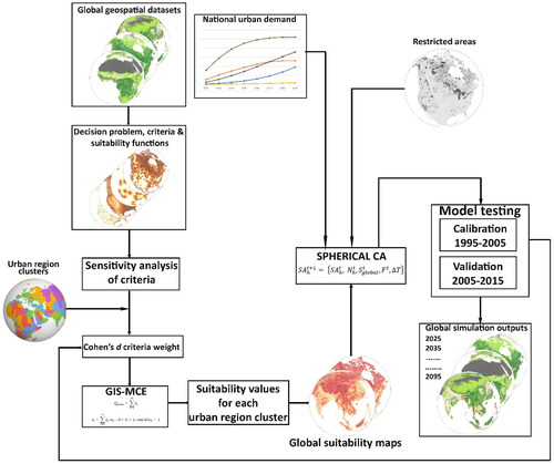
The second step comprises sensitivity analysis of selected criteria and classification of urban regions into clusters based on their similarities. Sensitivity analysis was performed to evaluate the influence of the selected criteria on overall suitability analysis. Global urbanization is characterized by diverse dynamics of various regions represented by different criteria that need different preferences. The clustering was used to identify urban regions with similar characteristics and then grouped into urban region clusters to enhance the suitability analysis.

The third step involves implementing GIS-MCE by generating criteria weights that reflect the relative importance of each criterion in the decision-making process. Given that actual stakeholders were not involved in this process, Cohen’s d criteria weight method has been applied to derive the values for the weights. Within the hexagonal data framework, criteria and weights were standardized to obtain the overall suitability values. The analysis is performed for each urban region cluster and combined to form the global suitability map which is then used as input to the spherical cellular automata (S-CA) model.

In the fourth step, the model is evaluated and then implemented to simulate urban land-use change. The temporal resolution of the model was determined to be 10 years based on the time interval of the available land-use datasets used in building and evaluating the model. This time period is also adequate to monitor and quantify the urban land-use change across the globe. Model evaluation comprises calibration using datasets for year 1995 and 2005 and validation using 2005 and 2015 data. For the period from 2015 to 2095 with each iteration corresponding to 10 years, the S-CA model generates the simulation outputs of urban land-use change based on obtained suitability values and considering national urban demand data and protected regions as constraints. The detailed description of each step of the proposed MCE-S-CA model is presented in the following sub-sections.

2.3. Selection of criteria and suitability functions

The identified criteria for this research study can be classified into three groups: socio-economic, biophysical, and proximity. Table 1 presents all selected criteria and their respective suitability functions in vertex notation and for GIS data layers with hexagonal cells. Suitability function values span from 0 to 1, where 1 indicate a full satisfaction for a criterion and 0 no satisfaction. Figure 2 was generated to present the spherical maps for all the criteria however depicted only for North America due to simplicity reasons. For each criterion, locations with maximum suitability are indicated in darker shades of brown while unsuitable locations are depicted in light brown.

Figure 2. Criterion maps of North America only and based on suitability functions for each criterion: (a) GDP, (b) Population density, (c) Slope, (d) Elevation, (e) Proximity to coast & inland water bodies, (f) Proximity to commercial areas, (g) Proximity to existing urban areas, and (h) Proximity to major roads.

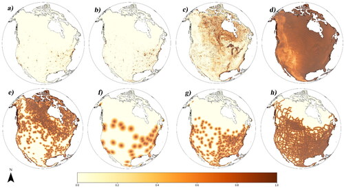
Table 1. Identified criteria and their respective suitability functions in vertex notation with justifications.

Group	Criteria	Suitability functions	Units	Justifications
Socio-economic	Gross domestic product (GDP)	GDP = [(816,1), (0,0)]	Million dollars per cell	Higher economic development boosts further urban development (Mahtta et al. 2022)
	Population density	Population = [(64161,1), (0,0)]	Inhabitants per cell	New urban development generally occurs closer to densely populated areas (Li and Cao 2019)
Biophysical	Slope	Slope = [(5,1), (50,0)]	Degrees	Areas with gentle slopes are preferred for urban development (Yan et al. 2020)
	Elevation	Elevation = [(100,1), (4000,0)]	Metres	Areas at lower elevation are more suitable for urban development (Mohamed and Worku 2020)
Proximity	Proximity to coast & inland water bodies	Water = [(0.99,1), (4.95,0)]	Kilometres	Water bodies provide scenic views and recreational activities (Zhao et al. 2021)
	Proximity to commercial areas	Commercial = [(0.99,1), (9.9,0)]	Kilometres	Proximity to commercial areas provides economic services and opportunities (Musa et al. 2019)
	Proximity to existing urban areas	Urban = [(0.99,1), (4.95, 0)]	Kilometres	Urban expansion typically occurs in proximity to existing urban development (Rimal et al. 2018)
	Proximity to major roads	Road = [(0.99, 1), (5.94, 0)]	Kilometres	Connection to transportation networks enhances urban development (Yang et al. 2018)

The socio-economic criteria consist of gross domestic product (GDP) and population density. The maximum and minimum values were utilized in developing the GDP and population density suitability functions based on previous studies (Feng et al. 2019; Zhang et al. 2020) that applied socio-economic criteria for analyzing urban development suitability. Economic factors are a major determinant of urban development and high GDP is often used as an indicator for high economic activities (He et al. 2014). Areas with high economic activities provide job opportunities as well as financial capital for urban development, thus there is a strong correlation between economic development and urban expansion (Mahtta et al. 2022). The GDP suitability function (Figure 2a) is expressed as a linear membership where locations of highest satisfaction are for a value of 816 million dollars per cell which represents the maximum GDP value obtained from the available GDP data. High population density creates high demand for urban development and are often preferred for future development by urban developers (Kim et al. 2020; Wu et al. 2021). These areas also indicate existing support for urban land development. New urban development tends to occur in and around densely populated areas (Bagan and Yamagata 2015). The population density suitability function utilizes a linear membership based on the obtained maximum value from the available data which is 64,161 inhabitants per hexagonal cell (Figure 2b).

Within the biophysical group are slope and elevation criteria. These two criteria can provide physical limitations to urban development. Generally, flat and gentle slopes are more prone to have urban development as it demands less cost and susceptible to surface run-off and soil erosion (Steiner et al. 2000; Zhou et al. 2021). For the slope suitability function (Figure 2c), gradients less than 5° yield maximum satisfaction and slopes steeper than 50° are considered unsuitable. Elevation can influence urban development especially in regions with rugged terrain. Urban development in higher elevation areas increases cost of construction and transportation. Generally, majority of urban development worldwide occurs in areas with lower elevation (Kii and Nakamura 2017). However, there are selected cities in high elevation for example Calgary, Canada, Denver, US, La Paz, Bolivia, Quito, Ecuador, Bogota, Columbia, and Addis Ababa, Ethiopia, thus they are taken into consideration for the choice of 4,000 m as the maximum elevation. The suitability function (Figure 2d) is fully satisfied in locations where elevation is less than 100 m and decreases with increasing elevation after 100 m with no satisfaction above 4,000 m.

The proximity criteria comprise proximity to coast & inland water bodies, commercial areas, existing urban areas, and major roads. Proximity to coast and inland water bodies provides natural scenery, good views, and opportunities for recreational and sporting activities (Zhao et al. 2021). New urban development typically occurs closer to these areas due to the services they offer (Cai et al. 2018). The approximated distance of 5 km was used as research suggests that services provided by water bodies decrease significantly after 5 km (Baró et al. 2016; Wen et al. 2017). The suitability function proximity to coast & inland water bodies (Figure 2e) has no satisfaction in locations within 0.99 km of coastline and water bodies due to the risk of flood. This distance is equivalent to one hexagonal cell in the spatial data layer. The suitability function has maximum satisfaction after 0.99 km and decreases monotonically with no satisfaction beyond 4.95 km which corresponds to five rings of hexagonal cells.

Jobs and employment opportunities are usually concentrated in the commercial areas of cities and also offer agglomeration advantages (Gharaibeh et al. 2020). People prefer to live closer to where they work to reduce the time and cost of commuting. Prior studies indicate compact urban growth is typically concentrated within 10 km distance of commercial areas (Cengiz et al. 2022). The proximity to commercial areas suitability function (Figure 2f) is fully satisfied in locations within 0.99 km of commercial areas and decreases with increasing distance with no satisfaction beyond 9.9 km that is represented by 10 hexagonal cells.

Proximity to existing urban areas criterion depict the influence of urban development process as the closer a parcel of land is to urban areas, the easier it is for developers to build new residential areas (Wu and Yeh 1997). Urban areas provide access to good road networks, already existing amenities, and commercial services among others (Bhatta 2010). Research confirms urban land develops near existing urban areas and 5 km is typically used as the maximum distance for suitability in urban land-use change studies (Rimal et al. 2018). The suitability function for proximity to existing urban areas (Figure 2g) is fully satisfied in locations within 0.99 km of existing urban areas and decreases after 0.99 km becoming unsuitable beyond 4.95 km while considering the size of the hexagons.

Major roads link urban areas together, boost fringe development and provide access to amenities, hence, urban development usually occurs in areas with access to major roads (Luo and Wei 2009). The chosen distance for the suitability function is based on studies by Yang et al. (2018) who indicated no significant change in urban development suitability beyond 6 km of major roads. The suitability function proximity to major roads (Figure 2h) yields maximum satisfaction in locations within 0.99 km of major roads and decreases gradually with no satisfaction after 5.94 km, and the distance is equivalent to six hexagonal cells.

2.4. Criteria sensitivity analysis and urban region clustering

Typically, sensitivity analysis examines the influence of input parameters on the model output variability (Saltelli et al. 2000). To determine the impact of individual criteria on overall suitability in different regions, criteria sensitivity test was performed using global sensitivity analysis (Ligmann-Zielinska and Jankowski 2014). The technique computes sensitivity and uncertainly from suitability surfaces generated using Monte Carlo simulations and applies variance decomposition methods to allocate model variability to each criterion. Table 2 presents the results of the global sensitivity analysis for some selected urban regions with distinctive characteristics. Positive values characterize positive spatial linear correlation between criteria values and overall suitability while negative values describe an inverse relationship between the criteria and overall suitability. For example, it is revealed that overall suitability in cities such as London and Shanghai is influenced by socio-economic criteria whilst cities like New Delhi and Riyadh are shaped by proximity to existing urban areas.

Table 2. Obtained sensitivity values for all criteria in some selected urban regions.

Criteria	London	Shanghai	Quito	Riyadh	Moscow	New Delhi	Indianapolis
GDP	0.279	0.176	0.333	0.454	0.366	0.208	0.425
Population density	0.196	0.202	0.182	0.294	0.193	0.034	0.305
Slope	0.039	0.076	0.056	0.012	−0.106	−0.069	0.016
Elevation	−0.006	−0.058	0.612	0.044	−0.089	0.092	0.282
Proximity to coast & inland water bodies	0.102	0.114	0.125	−0.049	0.262	−0.103	0.134
Proximity to commercial areas	0.164	0.203	0.676	0.688	0.417	0.218	0.472
Proximity to existing urban areas	0.209	0.056	0.655	0.705	0.661	0.543	0.470
Proximity to major roads	0.067	0.079	0.347	0.357	0.268	0.136	0.315

While urban development is influenced by similar criteria across different regions, the degree of influence varies. For this reason, there was the need to perform clustering analysis of urban regions to capture the specific similarities within them. The aim is to minimize the differences between urban regions in the same cluster while maximizing differences between the clusters. The world region was divided into 1860 sub-areas based on the location of existing cities with population greater than 300,000 inhabitants as per data from 2018 of the United Nations Department of Economic and Social Affairs (UN-DESA 2020). The k-means clustering technique (Jain 2010) was used due to its ability to specify number of clusters (k) suitable for the purpose of this study. Too many or too few clusters would not capture the main characteristics of urban regions. Therefore, four clusters have been chosen to group the sub-areas based on similarities related to their biophysical and socioeconomic characteristics. The resulting clusters as global maps are presented in Figure 3.

Figure 3. Results of urban region classification into four clusters based on their characteristics.

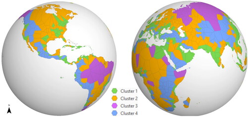
Cluster 1 consists of urban regions with high population density and GDP, located mainly along the coast or major water bodies consisting of metropolitan areas such as London, New York, Tokyo, Shanghai, Sao Paulo, Los Angeles, and Paris. Cluster 2 represents urban regions with average population density and GDP in low elevation urban regions like Montreal, Houston, Melbourne, Abidjan, and New Orleans. Cluster 3 characterizes urban regions with low population density and GDP in isolated locations such as Brisbane, Anchorage, Manaus, and Niamey. Cluster 4 comprises inland urban regions with average population density and GDP in areas with high elevation including Denver, Brasilia, Johannesburg, Riyadh, Calgary, and Quito.

2.5. Criterion weights and GIS-MCE technique

Criterion weights are generated to reflect the relative influence of each criterion on suitability for urban development. In most GIS-based MCE methods, weights are generally determined by subject experts or stakeholders. Given that this research study addresses the first global MCE-CA urban land-use change model and due to lack of resources, it was however not possible to elicit the opinions of various stakeholders and interest groups. Thus, criterion weights were generated for each urban region cluster using the Automatic Weight Selection technique (Veronesi et al. 2017). The technique uses statistical analysis based on the comparison between randomly sampled cells from spatial data layer representing the selected criteria and urban land-use type cells within each urban region cluster from the land-use data layer. From these two data layers, the Cohen’s d (Cohen 1988) values are computed for each criterion. The generated Cohen’s d values are normalized so their sum is equal to 1. This technique is applied to obtain the criterion weights for each urban region cluster and the obtained values are presented in Table 3.

Table 3. Criterion weights based on Cohen’s d for the four urban region clusters.

	Criteria weight for urban region
Criteria	Cluster 1	Cluster 2	Cluster 3	Cluster 4
GDP	0.1894	0.2554	0.2169	0.2211
Population density	0.1259	0.1108	0.1639	0.1166
Slope	0.0159	0.0135	0.0834	0.0527
Elevation	0.0936	0.0744	0.0870	0.0595
Proximity to coast & inland water bodies	0.0990	0.0984	0.1187	0.0097
Proximity to commercial areas	0.1632	0.0912	0.0099	0.1875
Proximity to existing urban areas	0.2055	0.2213	0.1979	0.2223
Proximity to major roads	0.1074	0.1351	0.1224	0.1308

The final step entails calculating the suitability value of each hexagonal cell using the GIS-MCE method. Overall suitability value for each hexagonal cell at the global level $S_{\mathit{global}}^t \text{at time} t$ can be calculated as sum of suitability values $S_i$ for each hexagonal cell of urban region cluster i (i = 1,…, m) and is based on weighted linear combination (WLC) approach as follows: (1) $$S_{\mathit{global}}^t=\mathrm{ }\sum _{i=1}^m{S}_i S_i=\mathrm{ }\sum _{j=1}^n{S}_{ji}\mathrm{ }{w}_{ji}\mathrm{ };\mathrm{ }0<S_i<1;\text{ sum of }{w}_{ji}=\mathrm{ }1$$(1) where $S_{ji}$ is the standardized criterion value based on suitability function transforming the input value of the criterion j (j = 1,…, n), n denotes number of criteria, m is number of urban region clusters and $w_{ji}$ 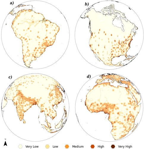is the weight of importance assigned to criterion j and urban region cluster i. The generated urban development suitability values are classified using equal interval method into five classes such as: very low (0–0.2), low (0.21–0.4), medium (0.41–0.6), high (0.61–0.8), and very high (0.81–1). Figure 4 presents the global suitability output displayed as spherical maps for each part of the Earth.

Figure 4. Resulting MCE suitability maps at global level for (a) South America, (b) North America, (c) Asia, and (d) Europe and Africa.

2.6. Spherical CA model

The spherical cellular automata part of the model (Figure 1) is designed to simulate urban land-use change by integrating the GIS-MCE component and the obtained suitability values as model input, and the constrains related to protected areas and national urban demand. The spherical automata SA comprises of an array of hexagonal cells h covering the Earth surface characterized with their states ${SA}_h^{t+1}$ at time t + 1 and expressed as: (2) $${SA}_h^{t+1}=\mathrm{ }\left\{{SA}_h^t,\mathrm{ }{\mathrm{ }N}_h^t,\mathrm{ }{S}_{\mathit{global}}^t,F^t,\Delta T\right\}$$(2) where ${SA}_h^t$ denotes the state of the hexagonal cell at initial time t, $N_h^t$ represents the hexagonal neighbourhood around the central cell, $S_{\mathit{global}}^t$ is the overall suitability value obtained from the GIS-MCE component of the model for each hexagonal cell, $F^t$ is the function of transition rules, and $\Delta T$ is the time step of one iteration.

A total of eight iterations of the model are run to simulate new urban development between 2015 $(T_i)$ and 2095 ($T_{i+8}$) where each iteration corresponds to a temporal resolution of 10 years. During each iteration, existing urban cells remain unchanged as well as protected areas and water bodies. The MCE-S-CA modelling approach is also constrained by national urban demand. The national urban demand is computed using GDP and population data obtained from UN-DESA (UN-DESA 2020) and Organization for Economic Co-operation and Development (OECD) (Dellink et al. 2017), respectively. The model iteratively simulates new urban development until the urban demand for each country has been reached. After each iteration, the S-CA model output becomes the input for the GIS-MCE component of the modelling framework, recalculates the suitability values based on new simulated urban development, and uses the updated information for the next model iteration and application of transition rules. The proposed MCE-S-CA model was programmed in Python (v3.7.7) (Van Rossum and Drake 2009) using DGGRID and H3 DGGS python libraries that are capable of generating and manipulating hexagonal cells covering the spherical Earth surface.

2.7. Model evaluation

Model evaluation comprises verification, calibration, and validation. Model verification entails ensuring the model’s logic and operations are correct and internally consistent, calibration involves adjusting model parameters whereas model validation often requires comparing the model output with independent datasets not used in building the model (Rykiel 1996; Manson 2007). Verification was conducted during the model design and implementation phase to ensure the logic and output of the code used is correct and testing the model after each modification and improvement to ensure it is consistent with the theory of the modelled process. The model was calibrated using historical dataset for the year 1995 and 2005. In the calibration phase, parameters representing transition rules are adjusted to allow for meaningful simulation of urban land-use change process. Model validation was performed using datasets for the year 2015, which represents data that have not been used in the model development and calibration phase. The simulation outputs were compared against actual land-use data using the Figure of Merit (FoM) approach (Pontius et al. 2008) which is the ratio of the intersection of simulated and observed change over the union of simulated and observed change and can be expressed as: (3) $$\mathit{FoM}=\mathrm{ }\frac{V}{U+V+W}$$(3) where V is the number of correctly simulated urban cells, U denotes the number of actual urban cells simulated as non-urban cells, and W is the number of non-urban cells simulated as urban cells. The FoM index constitutes three components considering only one class, urban land-use, was modelled with urban cells remaining unchanged in this research studies.

3. Results

3.1. Model testing

For the calibration phase, the FoM value obtained from the MCE-S-CA model was 51.1%, which is better than the 38% obtained for the S-CA model. The integration of MCE into the proposed model increased the FoM value by 13%. A comparison of these two models indicates the significance of operationalizing geosimulation models with MCE to enhance the abilities of function of transition rules. The FoM value for the MCE-S-CA model in the validation phase was 62.3%. The calculated FoM values from the proposed MCE-S-CA model were relatively higher than the values obtained in other global urban land-use change models found in the scientific literature with FoM validation figures ranging between 19% to 43% (Li et al. 2017; Cao et al. 2019; Chen et al. 2020; Li et al. 2021).

3.2. Global overview of urban expansion dynamics

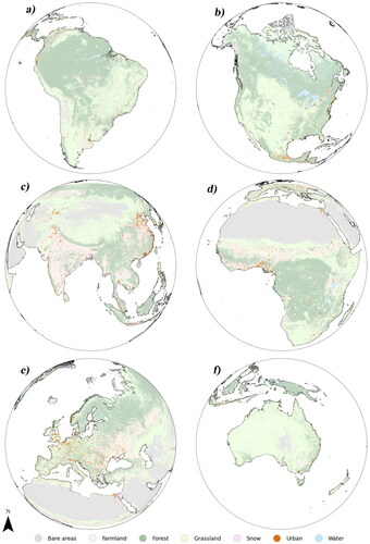
The simulation results indicate urban expansion altogether at the global scale would be rapid and extensive. Figure 5 presents the obtained global urban expansion simulation results for 2095 and for different parts of the world as spherical maps. The total global urban extent in 2015 was 747 thousand km² and this increased to 2.12 million km² in 2095. This corresponds to a global urban expansion of 1.37 million km² and an annual growth rate of 1.31% between 2015 and 2095. Although urban expansion is noticeable across all regions, the rate and size of urban growth in developing regions especially in Asia and Africa are relatively higher.

Figure 5. Obtained simulation results of global urban expansion for year 2095 in (a) South America, (b) North America, (c) Asia, (d) Africa, (e) Europe, and (f) Australia.

3.3. Variations in urban expansion across different urban region clusters

At the metropolitan level, differences in the simulated urban growth patterns can be observed across the four urban region clusters. The simulation results indicate cluster 1 urban regions which typically have high GDP and population density would collectively have the largest urban extent by the end of the century. The urban extent of metropolitan regions in cluster 1 increased from 488 thousand km² in 2015 to 1.37 million km² in 2095. This value represents an urban expansion of 880 thousand km² or 180% of urban growth. The annual growth rate of 1.3% is however slightly lower than the global rate. Urban growth in cluster 2 urban regions characterized by average GDP and population density in low lying regions was also considerable with the total urban extent increasing from 160 thousand km² in 2015 to 417 thousand km² in 2095. Between 2015 and 2095, the total urban extent in cluster 2 urban regions expanded by 161% with an annual growth rate of 1.21%. The total size of urban areas in metropolitan regions classified as cluster 3 which are in isolated regions with low GDP and population density was 11 thousand km² in 2015 and increased to 20 thousand km² in 2095. This represents the smallest urban growth rate and extent among the four urban region clusters. Urban areas in cluster 3 regions expanded by 79% with an annual growth rate of 0.73% in the period from 2015 to 2095. On the contrary, metropolitan areas in high-elevation areas with average GDP and population density termed cluster 4 urban regions had the highest urban growth rate of 248% and an annual growth rate of 1.57%. The total urban extent of cluster 4 urban regions increased from 89 thousand km² in 2015 to 310 thousand km² in 2095.

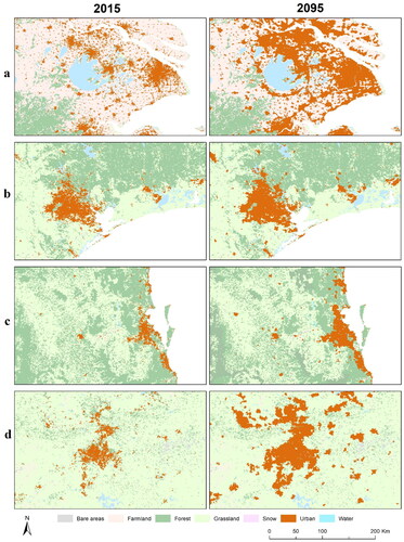
The simulation results of spatial urban expansion between 2015 and 2095 are presented in Figure 6 for different metropolitan areas as examples of urban areas that are indicated to have the most rapid urbanization in the four urban region clusters. The simulation results also indicate 64.4% of the total global urban expansion in the period between 2015 and 2095 would occur in cluster 1 metropolitan regions. Further, urban regions in clusters 2 and 4 would account for 18.8% and 16.2% of new urban development, respectively. However, less than 1% of the global urban expansion between 2015 and 2095 would occur in cluster 3 urban regions.

Figure 6. Comparison between 2015 urban land extent and obtained simulation results for 2095 for (a) Cluster 1, Shanghai, China, (b), Cluster 2, Houston, USA, (c) Cluster 3, Brisbane Australia, and (d) Cluster 4 Johannesburg, South Africa.

While the simulation results show a general trend of increased urban expansion among the four urban region clusters, differences in growth rates and urban land size can also be observed across continents. For example, the urban extent of cluster 2 metropolitan regions in Africa and Asia expanded by 606% and 395%, respectively, while urban areas in cluster 2 urban regions in Europe and North America increased by 65% and 67%, respectively. Also, by 2095, Asia would account for 52.7% of the total urban extent in metropolitan areas classified as cluster 1 urban regions. In contrast, Europe and North America would account for 19% and 10.3%, respectively, of the total urban extent within cluster 1 urban regions. The simulation results also revealed more urban growth would occur in cluster 1 urban regions across all continents albeit at different rates. For instance, 72% and 76% of total urban expansion in Asia and Europe would occur in cluster 1 urban regions, respectively. In North and South America, 55% and 41% of new urban development between 2015 and 2095 would be in cluster 1 urban regions.

4. Discussion and conclusions

The MCE-S-CA model presented in this research study can realistically represent and capture urban growth dynamics across the globe as indicated by the relatively better FoM values obtained during model evaluation. Also, the simulated results from the proposed model are comparable to other global urban land-use change simulations and studies. The simulation outputs indicate the total global urban extent would exceed 2.1 million km² by the end of the twenty-first century. This is consistent with other global land-use change studies such as Li et al. (2019) who projected the total urban extent by the year 2100 to be 2.4 million km² in their studies. Africa and Asia would become the frontier of urban expansion and are indicated to have the highest urban expansion rate and largest new urban land size by 2095. The high urban expansion rates observed in developing regions especially in Africa and Asia also correspond to research findings by Li et al. (2021).

Cities are engines of economic growth and human innovation and are expected to play considerable roles in ensuring a globally sustainable future in the coming decades. This is especially true for large global cities that dominate social and economic interactions across the globe. Studies indicate a close correlation between urbanization and economic growth (Chen et al. 2014). The simulation results indicate cluster 1 urban regions which have distinctively high GDP and population density would account for 64% of the total global urban expansion between 2015 and 2095. This trend is observable across all geographic regions and by the end of the century, cluster 1 urban regions have the largest urban extent within each continent except for Australia and Oceania. Also, by the end of the twenty-first century, 84.4% of the total global urban extent would be in cluster 1 and 2 urban regions. Metropolitan areas in these two urban clusters are typically located in low-lying coastal areas and along major water bodies thus most at risk of the consequences of climate change including sea level rise and flooding. With several developing countries still in the initial phase of urbanization, cities can still shape the future of urbanization in these regions through sustainable urban policies and regional development strategies to limit the negative impacts of rapid urbanization. Cities in Asia and Africa for example would account for 72% of new urban-land development between 2015 and 2095.

The research study has some limitations, and the implemented model can further be enhanced. Firstly, the proposed model does not incorporate random effects for some variables due to lack of data to derive probabilities and computational capacity to run the model at global extent multiple times to examine the convergence. Secondly, the model does not account for the effects of potential human-induced changes such as future development of infrastructure of network of new highways or railways, increased economic activities of port cities, deforestation and agricultural land degradation or environmental changes ranging from natural hazards such as earthquakes and forest fires to climate change and sea level rise that can affect urban land use change. Also, the urban development suitability analysis can be improved by including other relevant criteria in the analysis such as local-level planning and policies, land value, climate variables or scenarios among others. Incorporating the participation of stakeholders and subject experts would be beneficial to appropriately determine the selection of criteria and importance of criterion weights. This would then require the use of advanced spatial decision techniques such as the Logic Scoring of Preference (LSP) method within the CA framework, that are capable of handling larger number of criteria based on soft computing logic. In addition, future research works would focus on representation and comparison of planer and spherical geospatial data to quantify and analyze the source of errors and differences in model outputs. Despite these drawbacks, the proposed geosimulation model is flexible and has the capability to be utilized to explore multiple environmental and urban development scenarios that can be postulated by different stakeholders, experts, and policymakers within the scope of global urban planning and management procedures.

In conclusion, this research study presents a novel MCE-S-CA geosimulation approach for simulating global urban land-use change by considering the curvature of the global Earth surface. The proposed modelling approach provides decision-making capabilities that can represent different urban development criteria and preferences across diverse metropolitan regions at the global level. The model is capable of analyzing and identifying suitable locations for urban development and simulating urban land-use change across different global urban regions.

Acknowledgements

The authors are thankful for the support of this study by the Natural Sciences and Engineering Research Council of Canada (NSERC) and the Simon Fraser University (SFU) Graduate Dean’s Entrance Scholarship (GDES). The authors are also grateful for support provided by the SFU Open Access Fund. This research was also partly enabled by support provided by Compute Canada and WestGrid high performance comping facilities. The authors also thank the three anonymous reviewers for their valuable and constructive feedback.

Disclosure statement

The authors declare no conflict of interest.

Data availability statement

Data supporting the findings of this study are available from the corresponding author on request.

Additional information

Funding

This research was funded by the Natural Sciences and Engineering Research Council of Canada (NSERC) Discovery Grant [RGPIN-2017-03939] awarded to the second author.

References

- Bagan H, Yamagata Y. 2015. Analysis of urban growth and estimating population density using satellite images of nighttime lights and land-use and population data. GISci Remote Sens. 52(6):765–780.
- Baró F, Palomo I, Zulian G, Vizcaino P, Haase D, Gómez-Baggethun E. 2016. Mapping ecosystem service capacity, flow and demand for landscape and urban planning: a case study in the Barcelona metropolitan region. Land Use Policy. 57:405–417.
- Bhatta B. 2010. Causes and consequences of urban growth and sprawl. In: Bhatta B, editor, Analysis of urban growth and sprawl from remote sensing data; Berlin: Springer; p. 17–36.
- Cai Z, Han G, Chen M. 2018. Do water bodies play an important role in the relationship between urban form and land surface temperature? Sustain Cities Soc. 39:487–498.
- Cao K, Huang B, Li M, Li W. 2014. Calibrating a cellular automata model for understanding rural-urban land conversion: a Pareto front-based multi-objective optimization approach. Int J Geogr Inform Sci. 28(5):1028–1046.
- Cao M, Zhu Y, Quan J, Zhou S, Lü G, Chen M, Huang M. 2019. Spatial sequential modeling and predication of global land use and land cover changes by integrating a global change assessment model and cellular automata. Earth’s Future. 7(9):1102–1116.
- Cengiz S, Görmüş S, Oğuz D. 2022. Analysis of the urban growth pattern through spatial metrics; Ankara City. Land Use Policy. 112:105812.
- Chen M,Zhang H,Liu W,Zhang W. 2014. The global pattern of urbanization and economic growth: Evidence from the last three decade. PLoS One. 9(8):e103799.
- Chen G, Li X, Liu X. 2022. Global land projection based on plant functional types with a 1-km resolution under socio-climatic scenarios. Sci Data. 9(1):1–18.
- Chen G, Li X, Liu X, Chen Y, Liang X, Leng J, Xu X, Liao W, Qiu Y, Wu a, et al. 2020. Global projections of future urban land expansion under shared socioeconomic pathways. Nat Commun. 11(1):537.
- Cohen J. 1988. Statistical power analysis for the behavioral sciences. New York: Routledge.
- de Sousa LM, Poggio L, Kempen B. 2019. Comparison of FOSS4G supported equal-area projections using discrete distortion indicatrices. IJGI. 8(8):351.
- Dellink R, Chateau J, Lanzi E, Magné B. 2017. Long-term economic growth projections in the Shared Socioeconomic Pathways. Global Environ Change. 42:200–214.
- Ellis EC, Gauthier N, Klein Goldewijk K, Bliege Bird R, Boivin N, Díaz S, Fuller DQ, Gill JL, Kaplan JO, Kingston N, et al. 2021. People have shaped most of terrestrial nature for at least 12,000 years. Proc Natl Acad Sci USA. 118(17):e2023483118.
- European Space Agency. 2017. Land Cover CCI Product User Guide Version 2. Tech. Rep. [accessed 2019 November 10. http://maps.elie.ucl.ac.be/CCI/viewer/download/ESACCI-LC-Ph2-PUGv2_2.0.pdf.
- Feng Y, Wang J, Tong X, Shafizadeh-Moghadam H, Cai Z, Chen S, Lei Z, Gao C. 2019. Urban expansion simulation and scenario prediction using cellular automata: comparison between individual and multiple influencing factors. Environ Monit Assess. 191(5):291.
- Gao J, O'Neill BC. 2019. Data-driven spatial modeling of global long-term urban land development: the SELECT model. Environ Modell Software. 119:458–471.
- Gharaibeh A, Shaamala A, Obeidat R, Al-Kofahi S. 2020. Improving land-use change modeling by integrating ANN with cellular automata-Markov Chain model. Heliyon. 6(9):e05092.
- Ghosh T, Powell RL, Elvidge CD, Baugh KE, Sutton PC, Anderson S. 2011. Shedding light on the global distribution of economic activity. Open Geogr J. 3:148–161.
- Hall J, Wecker L, Ulmer B, Samavati F. 2020. Disdyakis triacontahedron DGGS. IJGI. 9(5):315.
- He C, Huang Z, Wang R. 2014. Land use change and economic growth in urban China: a structural equation analysis. Urban Stud. 51(13):2880–2898.
- Hojati M, Robertson C, Roberts S, Chaudhuri C. 2022. GIScience research challenges for realizing discrete global grid systems as a Digital Earth. Big Earth Data. 6(3):358–379.
- Iovine G, D'Ambrosio D, Di Gregorio S. 2005. Applying genetic algorithms for calibrating a hexagonal cellular automata model for the simulation of debris flows characterised by strong inertial effects. Geomorphology. 66(1–4):287–303.
- Jain AK. 2010. Data clustering: 50 years beyond K-means. Pattern Recogn Lett. 31(8):651–666. Elsevier B.V.
- Kiester AR, Sahr K. 2008. Planar and spherical hierarchical, multi-resolution cellular automata. Comput Environ Urban Syst. 32(3):204–213.
- Kii M, Nakamura K. 2017. Development of a suitability model for estimation of global urban land cover. Transp Res Procedia. 25:3161–3173.
- Kim Y, Newman G, Güneralp B. 2020. A review of driving factors, scenarios, and topics in urban land change models. Land. 9(8):246.
- Li X,Zhou Y,Eom J,Yu S,Asrar GR. 2019. Projecting Global Urban Area Growth Through 2100 Based on Historical Time Series Data and Future Shared Socioeconomic Pathways. Earth's Future. 7(4):351–362.
- Li P, Cao H. 2019. Simulating uneven urban spatial expansion under various land protection strategies: case study on southern Jiangsu urban agglomeration. IJGI. 8(11):521.
- Li X, Chen G, Liu X, Liang X, Wang S, Chen Y, Pei F, Xu X. 2017. A new global Land-use and land-Cover change product at a 1-km resolution for 2010 to 2100 based on human–environment interactions. Ann Am Assoc Geographers. 107(5):1040–1059.
- Ligmann-Zielinska A, Jankowski P. 2014. Spatially-explicit integrated uncertainty and sensitivity analysis of criteria weights in multicriteria land suitability evaluation. Environ Modell Software. 57(2014):235–247.
- Li M, Stefanakis E. 2020. Geospatial operations of discrete global grid systems—a Comparison with traditional GIS. J Geovis Spat Anal. 4(2):1–21.
- Li X, Yu L, Sohl T, Clinton N, Li W, Zhu Z, Liu X, Gong P. 2016. A cellular automata downscaling based 1 km global land use datasets (2010–2100). Science Bulletin. 61(21):1651–1661.
- Li X, Zhou Y, Hejazi M, Wise M, Vernon C, Iyer G, Chen W. 2021. Global urban growth between 1870 and 2100 from integrated high resolution mapped data and urban dynamic modeling. Commun Earth Environ. 2(1):1–10.
- Luo J, Wei YHD. 2009. Modeling spatial variations of urban growth patterns in Chinese cities: the case of Nanjing. Landscape Urban Plann. 91(2):51–64.
- Mahtta R, Fragkias M, Güneralp B, Mahendra A, Reba M, Wentz EA, Seto KC. 2022. Urban land expansion: the role of population and economic growth for 300+ cities. Npj Urban Sustain. 2(5):1–11.
- Malczewski J. 1996. A GIS-based approach to multiple criteria group decision-making. Int J Geogr Inform Syst. 10(8):955–971.
- Malczewski J, Jankowski P. 2020. Emerging trends and research frontiers in spatial multicriteria analysis. Int J Geogr Inform Sci. 34(7):1257–1282.
- Manson SM. 2007. Challenges in evaluating models of geographic complexity. Environ Plan B Plan Des. 34(2):245–260.
- Masoudi M, Centeri C, Jakab G, Nel L, Mojtahedi M. 2021. GIS-based multi-criteria and multi-objective evaluation for sustainable land-use planning (case study: Qaleh Ganj County, Iran) “Landuse planning using MCE and Mola”. Int J Environ Res. 15(3):457–474.
- Meijer JR, Huijbegts MAJ, Schotten CGJ, Schipper AM. 2018. Global patterns of current and future road infrastructure. www.globio.info.
- Mohamed A, Worku H. 2020. Simulating urban land use and cover dynamics using cellular automata and Markov chain approach in Addis Ababa and the surrounding. Urban Clim. 31(2020):100545.
- Musa SI, Hashim M, Reba MNM. 2019. Geospatial modelling of urban growth for sustainable development in the Niger Delta Region, Nigeria. Int J Remote Sens. 40(8):3076–3104.
- National Research Council. 2014. Advancing land change modeling: opportunities and research requirements. Washington (DC): The National Academies Press.
- Nugraha AT, Waterson BJ, Blainey SP, Nash FJ. 2021. On the consistency of urban cellular automata models based on hexagonal and square cells. Environ Plann B: urban Anal City Sci. 48(4):845–860.
- Nuissl H, Siedentop S. 2021. Urbanisation and land use change. In Weith T, Barkmann T, Gaasch N, Rogga S, Strauß C, Zscheischler J, editors, Sustainable land management in a European context: a co-design approach. Cham: springer; p. 75–99.
- Pontius RG, Boersma W, Castella J-C, Clarke K, de Nijs T, Dietzel C, Duan Z, Fotsing E, Goldstein N, Kok K, et al. 2008. Comparing the input, output, and validation maps for several models of land change. Ann Reg Sci. 42(1):11–37.
- Purss MBJ, Peterson PR, Strobl P, Dow C, Sabeur ZA, Gibb RG, Ben J. 2019. DataCubes: a discrete global grid systems perspective. Cartographica. 54(1):63–71. doi
- Rimal B, Zhang L, Keshtkar H, Haack BN, Rijal S, Zhang P. 2018. Land use/land cover dynamics and modeling of urban land expansion by the integration of cellular automata and Markov chain. IJGI. 7(4):154.
- Robertson C, Chaudhuri C, Hojati M, Roberts SA. 2020. An integrated environmental analytics system (IDEAS) based on a DGGS. ISPRS J Photogramm Remote Sens. 162:214–228.
- Rose AN, McKee JJ, Sims KM, Bright EA, Reith AE, Urban ML. 2020. LandScan 2019 [digital raster data]. https://landscan.ornl.gov/.
- Rykiel EJ. 1996. Testing ecological models: the meaning of validation. Ecol Modell. 90(3):229–244.
- Sahr K. 2011. Hexagonal discrete global GRID systems for geospatial computing. Arch Photogram Cartogr Remote Sens. 22:363–376.
- Saltelli A, Chan K, Scott M. 2000. Sensitivity analysis. In Probability and statistics series. New York: John Wiley & Sons.
- Seto KC, Güneralp B, Hutyra LR. 2012. Global forecasts of urban expansion to 2030 and direct impacts on biodiversity and carbon pools. Proc Natl Acad Sci USA. 109(40):16083–16088.
- Steiner F, McSherry L, Cohen J. 2000. Land suitability analysis for the upper Gila River watershed. Landscape Urban Plann. 50(4):199–214.
- Turner BL, Lambin EF, Verburg PH. 2021. From land-use/land-cover to land system science. Ambio. 50(7):1291–1294.
- United Nations – Department of Economic and Social Affairs: Population Division. 2020. World Population Prospects 2019. [accessed 2020 November 9] https://population.un.org/wpp/.
- United State Geological Survey 2020. USGS EROS Archive – Digital elevation – shuttle radar topography mission (SRTM) 1 arc-second global. [accessed 2020 August] https://www.usgs.gov/centers/eros/science/usgs-eros-archive-digital-elevation-shuttle-radar-topography-mission-srtm-1-arc?qt-science_center_objects=0#qt-science_center_objects.
- Van Rossum G, Drake F. 2009. Python 3 reference manual. Scotts Valley (CA): createSpace.
- Ventrella J. 2011. Glider dynamics on the sphere: exploring cellular automata on geodesic grids. J Cell Automata. 6:245–256.
- Verburg PH, Crossman N, Ellis EC, Heinimann A, Hostert P, Mertz O, Nagendra H, Sikor T, Erb KH, Golubiewski N, et al. 2015. Land system science and sustainable development of the earth system: a global land project perspective. Anthropocene. 12:29–41.
- Veronesi F, Schito J, Grassi S, Raubal M. 2017. Automatic selection of weights for GIS-based multicriteria decision analysis: site selection of transmission towers as a case study. Appl Geogr. 83:78–85.
- Wen H, Xiao Y, Zhang L. 2017. Spatial effect of river landscape on housing price: an empirical study on the Grand Canal in Hangzhou, China. Habitat Int. 63:34–44.
- Winkler K, Fuchs R, Rounsevell M, Herold M. 2021. Global land use changes are four times greater than previously estimated. Nat Commun. 12(1):1–10.
- World Database on Protected Areas. 2020. Global database on terrestrial and marine protected areas. [accessed 2020 March 4] https://www.protectedplanet.net/en/search-areas?filters%5Bdb_type%5D%5B%5D=wdpa&geo_type=region.
- Wu R, Li Z, Wang S. 2021. The varying driving forces of urban land expansion in China: insights from a spatial-temporal analysis. Sci Total Environ. 766:142591.
- Wu F, Webster CJ. 1998. Simulation of land development through the integration of cellular automata and multicriteria evaluation. Environ Plann B. 25(1):103–126.
- Wu F, Yeh AGO. 1997. Changing spatial distribution and determinants of land development in Chinese cities in the transition from a centrally planned economy to a socialist market economy: a case study of Guangzhou. Urban Stud. 34(11):1851–1879.
- Yan Y,Ju H,Zhang S,Jiang W. 2020. Spatiotemporal Patterns and Driving Forces of Urban Expansion in Coastal Areas: A Study on Urban Agglomeration in the Pearl River Delta, China. Sustainability. 12(1):191.
- Yang J, Liu W, Li Y, Li X, Ge Q. 2018. Simulating intraurban land use dynamics under multiple scenarios based on fuzzy cellular automata: a case study of Jinzhou district, Dalian. Complexity. 2018:1–17.
- Zhai X, Xiao Z, Yin P. 2010. Framework of cellular automaton on sphere. Paper presented at the ICCET 2010 – 2010 2nd International Conference on Computer Engineering and Technology, Proceedings.
- Zhang X, Zhou J, Song W. 2020. Simulating urban sprawl in China based on the artificial neural network-cellular Automata-Markov model. Sustainability. 12(11):4341.
- Zhao L, Li G, Yao X, Ma Y, Cao Q. 2022. An optimized hexagonal quadtree encoding and operation scheme for icosahedral hexagonal discrete global grid systems. Int J Digital Earth. 15(1):975–1000.
- Zhao W, Wang Y, Chen D, Wang L, Tang X. 2021. Exploring the influencing factors of the recreational utilization and evaluation of urban ecological protection green belts for urban renewal: a case study in Shanghai. IJERPH. 18(19):10244.
- Zhou L, Dang X, Mu H, Wang B, Wang S. 2021. Cities are going uphill: slope gradient analysis of urban expansion and its driving factors in China. Sci Total Environ. 775:145836.
- Zhou Y, Varquez ACG, Kanda M. 2019. High-resolution global urban growth projection based on multiple applications of the SLEUTH urban growth model. Sci Data. 6(1):10.