An enhanced spatiotemporal fusion model with degraded fine-resolution images via relativistic generative adversarial networks

Abstract

Limited by the sensor technology and budget, spatiotemporal fusion (STF) of remote sensing images (RSIs) is an effective strategy to obtain products with dense time and high spatial resolution. The STF methods generally require at least three observed images, and the predicted results depend on the reference date. The lack of high-quality fine-resolution images in practice makes the STF model difficult to apply, and few models consider the bias caused by different sensors. To solve the above problems, an enhanced STF model with degraded fine-resolution images via relativistic generative adversarial networks is proposed, called EDRGAN-STF, which is an end-to-end network with all bands trained simultaneously. To reduce the bias caused by different sensors, a degraded resolution version of the Landsat image with an arbitrary date is introduced into the STF model. The inputs of EDRGAN-STF only contain a MODIS image of the predicted date, a reference Landsat image and degraded version with an arbitrary date. EDRGAN-STF consists of a generator and a relativistic average least squares discriminator (RaLSD). A dual-stream residual dense block is designed to fully obtain the local and global spatial details and low-frequency information in the generator. A multihierarchical feature fusion block is designed to fuse global information. A spectral-spatial attention mechanism is employed in the generator, which focuses on important spectral bands and spatial features and enhances the reconstruction of critical regions. A new composite loss function is introduced to better optimize the designed STF model. To verify the capability of the EDRGAN-STF, extensive experiments are conducted on two typical Landsat-MODIS datasets, and results illustrate that EDRGAN-STF improves the STF accuracy and has great prospects for practical applications.

Key policy highlights:

1. The proposed EDRGAN-STF improves spatiotemporal fusion accuracy and has great prospects for practical applications.

2. A degraded resolution version of the Landsat image with an arbitrary date is introduced into the spatiotemporal fusion model.

3. A dual-stream residual dense block is designed to fully obtain the local and global spatial details and low-frequency information.

4. A spectral-spatial attention mechanism focuses on important spectral bands and spatial features and enhances the reconstruction of critical regions.

5. A multihierarchical feature fusion block fuses global information and a new composite loss function is introduced to better optimize the model.

Keywords:

• Relativistic average least squares generative adversarial networks (RaLSGAN)
• dual-stream residual dense block
• multihierarchical feature fusion
• remote sensing images
• spatiotemporal fusion

1. Introduction

Remote sensing images (RSIs) with dense time and high spatial resolution have been widely used in monitoring of phenology, urban and Earth resources, dynamic changes of ecological environment and warnings of disaster (Zhu et al. 2022). However, limited by the sensor technology and budget, RSIs with both high temporal and high spatial resolution (HTHS) cannot be obtained (Zhou et al. 2021; Zhu et al. 2022). The spatiotemporal fusion (STF) is one of the more convenient methods to obtain HTHS images (Zhou et al. 2021). The STF technology employs low temporal and high spatial resolution (LTHS) images and high temporal and low spatial resolution (HTLS) images to generate HTHS images (Zhou et al. 2021). Many researchers have studied STF techniques, which can be roughly divided into weight-based, unmixing-based, hybrid and learning-based STF methods (Li et al. 2020c; Zhu et al. 2022).

The most representative STF methods based on weight are as follows. Gao et al. (2006) designed a spatial and temporal adaptive reflectance fusion model (STARFM) fusing MODIS (HTLS) and Landsat (LTHS) images to generate HTHS images. STARFM uses three images as inputs, as described in Figure 1(a): one pair of HTLS-LTHS images on the reference date (C₀ and F₀) and an HTLS image of the predicted date (C₁). When predicting complex heterogeneous scenes and the target size is smaller than the coarse resolution, the prediction accuracy of the STARFM is limited. Subsequently, many scholars improved the STARFM method. Zhu et al. designed an enhanced STARFM (ESTARFM) method (Zhu et al. 2010). ESTARFM uses five images as inputs, as exhibited in Figure 1(b): two pairs of HTLS-LTHS images on the reference date (C₀ and F₀, C₂ and F₂) and one HTLS image of the predicted date (C₁). ESTARFM searches for similar pixels with all bands, uses spectral similarity (correlation coefficient) to calculate weights, and employs different conversion coefficients to improve prediction accuracy in heterogeneous regions. The difference between the weight-based STF methods lies in the method for calculating similar pixels and the method for calculating the weight of similar pixels. Since the weight-based models suppose that the changes in low-resolution images are the same as those of fine-resolution images, these methods are more challenging for predicting scenes with large changes in a short period of time.

Figure 1. Inputs of STF model. (a) One pair of HTLS-LTHS images on the reference date (C₀ and F₀), a HTLS image of the predicted date (C₁), and the predicted result PF₁. (b) Two pairs of HTLS-LTHS images on the reference date ((C₀, F₀) and (C₂, F₂)), and a HTLS image of the predicted date (C₁).

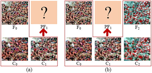
Zhukov et al. designed an unmixing-based multisensor multiresolution image fusion (UMMF) method (Zhukov et al. 1999). UMMF first performs spectral unmixing on the coarse-resolution image and replaces spectrum information of the high-resolution data according to the unmixing results to generate the predicted data. UMMF has errors in spectral unmixing and lacks endmember spectral invariance. Wu et al. improved UMMF and proposed a spatial temporal data fusion approach (STDFA) (Wu et al. 2012). STDFA considers the nonlinear temporal change similarity and spatial variation during the spectral unmixing. Nevertheless, unmixing-based techniques are still challenging for the prognostication of land-cover-type changes.

Hybrid STF methods have achieved promising results. Zhu et al. advanced a flexible spatiotemporal data fusion (FSDAF) method using the spectral unmixing analysis and thin plate spline (TPS) interpolation (Zhu et al. 2016). FSDAF first employs the unmixing method to generate a transitional image, then calculates and distributes residuals, and finally uses the weight-based method to acquire the predicted data. FSDAF is applicable to heterogeneous scenes and predicts gradual changes and land-cover-type changes, which requires three observed images. Liu et al. improved the FSDAF method, i.e. IFSDAF (Liu et al. 2019a). IFSDAF uses the constrained least squares to optimize the unmixed and TPS-interpolated increment to generate predicted images. IFSDAF is also suitable for fine-resolution images with clouds. Guo et al. (2020) presented an FSDAF 2.0 approach, which enhances the accuracy of products and strengthens the robustness of STF. Li et al. (2020b) designed an SFSDAF approach by combining the subpixel class fraction change information to minimize the image blurring and improve the prediction accuracy. Liu et al. (2022) proposed a spectral autocorrelation STF model (FIRST) for the spectral uncorrelation of available STF approaches. FIRST not only boosts the STF accuracy, but also is applicable to images with haze and thin clouds. Hou et al. (2022) proposed a robust FSDAF (RFSDAF) for image registration errors. RFSDAF adapts to different registration errors by introducing a multiscale fusion method to reduce the impact of registration errors on STF.

Learning-based STF methods have developed rapidly. Huang and Song (2012) introduced dictionary learning to STF and designed a sparse representation-based STF model (SPSTFM). SPSTFM establishes reflectance changes between low- and high-resolution images at the reference time using dictionary learning, and then predicts fine-resolution images on the predicted date. For a pair of prior images, Song and Huang (2013) proposed a one-pair image learning method based on the SPSTFM (SSIF). SSIF strengthens the coarse images through dictionary learning, and then a high-pass model fuses the above results with prior high-resolution images to generate predicted images. The generalization ability of dictionary learning to different scenarios is weak and needs to be learned again. Deep learning (DL) has good generalization ability, and DL is gradually applied in STF. Song et al. (2018) designed an approach via a deep convolutional neural network (CNN) for STF (STDCNN), which constructs the relationship between coarse- and fine-resolution images through the CNN, and then generates predicted images through a high-pass fusion block. Liu et al. (2019b) proposed a dual-stream CNN for STF (StfNet), which employs temporal dependencies and temporal consistency in image sequences during super-resolution. STDCNN and StfNet are not end-to-end STF models, and are trained band-by-band, increasing model complexity and training time. Tan et al. (2018, 2019) designed a deep CNN for STF (DCSTFN) and an enhanced DCSTFN (EDCSTFN). EDCSTFN extracts high-frequency features and changing features based on CNN to reconstruct high-resolution images of the predicted date and designs a composite loss function. Li et al. (2020c) proposed a sensor bias-driven STF model via CNN (BiaSTF), which considers sensor biases between MODIS and Landsat data to reduce spectral and spatial distortions. Li et al. (2022a) designed an STF approach via the linear regression (LiSTF), which fuses MODIS-like images with high-resolution images to reduce uncertainty errors and better preserve spatial information. Chen et al. (2022) proposed an STF model employing multiscale two-stream CNNs (STFMCNNs), which extracts features of objects with different sizes through multiscale convolution, and uses the temporal dependence and the temporal consistency to compensate information for STF. Li et al. (2022b) proposed a pseudo-siamese deep CNN (PDCNN) for STF. PDCNN contains two independent and equal feature extraction branches, which do not share weights. PDCNN improves the prediction accuracy through a multiscale mechanism, dilated convolutions, an attention mechanism, and residual connections. Li et al. (2021c) also designed a network based on an attention mechanism and a multiscale mechanism (AMNet), which uses one pair of images as prior data and is trained band-by-band. Ma et al. (2021) proposed a stepwise model for STF (SSTSTF), which establishes spatial, sensor and temporal difference models based on deep CNNs. The three difference models are trained separately and the entire STF model is complicated, which is not an end-to-end model. Zhang et al. (2021) designed a STF method employing generative adversarial networks (GAN), i.e. STFGAN, which is a two-stage framework, and each stage is an image fusion GAN (IFGAN) composed of residual blocks. The IFGAN is trained simultaneously on all bands, which reduces time and consumption. Shang et al. (2022) advanced an adaptive reflectance STF approach via a GAN for the problems that the STF models require two pairs of reference images, which are not applicable in practice, and the STF models are generally trained band-by-band without considering the spectral correlation. Tan et al. (2022) designed a model employing a conditional GAN and a switchable normalization technique for STF (GAN-STFM), which reduces the number of model inputs and breaks through the time interval limitation between reference and predicted images. The GAN-STFM only demands two observed images and has low requirements for time interval, which improves the application in practice.

The powerful nonlinearity of DL makes it applied in STF of RSIs, and there is still great room for improvement in the current STF technology. Most of the STF models are trained band-by-band, ignoring the information correlation between bands, which increases both time cost and computational cost. Affected by weather and clouds, there are few high-quality HTLS-LTHS image pairs observed, which cannot satisfy the DL model that requires a large amount of training data. At present, the STF model mostly employs at least one pair of reference data, which is difficult to apply in practice. In addition, the GAN-STFM (Tan et al. 2022) model takes a Landsat image with an arbitrary reference date (ARLI) and a MODIS image of the predicted date (PMI) as inputs to generate a Landsat image of the predicted date (PLI). Although GAN-STFM provides a more practical method, the method needs to be improved in the following aspects. First, the bias of the sensor leads to the information difference between the MODIS and Landsat images, the GAN-STFM only uses the PMI image to extract the spectral information, resulting in some spectral distortions in the generated Landsat image. Second, the GAN-STFM employs a simple residual structure to extract features, and RSIs contain rich information, which easily leads to insufficient features to express the information of RSIs. Third, the discriminator distinguishes the probability that the generated image is real or fake, which would reduce the probability that the real image is real (Jolicoeur-Martineau 2019), and then may cause some spectral and detail distortions.

To solve the above problems, an enhanced STF model with degraded fine-resolution images via relativistic generative adversarial networks is proposed, called EDRGAN-STF. The proposed EDRGAN-STF is an end-to-end network with three inputs: an ARLI, a degraded resolution version of ARLI (DARLI) and a PMI, which is trained simultaneously on all bands. Extensive experiments are conducted to validate the proposed EDRGAN-STF. The main contributions of this article are as follows.

• To reduce the bias caused by different sensors, a degraded resolution version of the Landsat image is introduced into the STF model. The DARLI and PMI are concatenated and fused to obtain adequate low-frequency information that is closer to the characteristics of Landsat products.

• A dual-stream residual dense block (DSRDB) in the generator is designed to more fully obtain local dense and global multihierarchical spatial details of the ARLI and multihierarchical low-frequency information of the DARLI and PMI.

• A dual-stream multihierarchical feature fusion block (MHFFB) is designed to fuse multihierarchical high-frequency details and low-frequency information from DSRDBs separately to extract the final global features.

• A new composite loss function is introduced to better optimize the designed STF model.

The other sections of the article are arranged as follows. Section 2 introduces related works. Section 3 details the proposed STF model and constructs a composite loss function. Section 4 presents data sets, evaluation indices, compared experiments and ablation experiments. Section 5 is discussions. Section 6 comes to conclusions.

2. Related works

2.1. GAN

Goodfellow et al. (2014) designed a standard GAN (SGAN) containing a generator (G) and discriminator (D). When training G and D concurrently, a minimax two-player game between G and D is constructed; D distinguishes between real and fake data and G generates fake data as much as possible as real data, making D cannot distinguish between the real data and the generated fake data. Wasserstein GAN (WGAN) optimizes a reasonable and efficient approximation of the Wasserstein distance to solve the SGAN model collapse problem, but the convergence speed is relatively slow (Arjovsky et al. 2017). Least squares GAN (LSGAN) uses the least squares loss function to solve the vanishing gradient problem caused by the cross-entropy loss function of SGAN (Mao et al. 2017). The image quality generated by LSGAN is higher than that of SGAN, the performance is more stable, and it is easier to converge than WGAN. The D of SGAN (SD) directly distinguishes whether the data are true or false. Relativistic average GAN (RaGAN) improves the optimization objective of the SD using a relativistic average discriminator (RaD) to estimate the probability that the given real sample is more realistic than the fake sample, on average, and the probability that the fake sample is more realistic than the real sample, on average (Jolicoeur-Martineau 2019). RaGAN improves the SGAN performance and stability without increasing the computational cost. Spectrally normalized GAN (SNGAN) employs a spectral normalization (SpN) technique to enhance the discriminator stability (Miyato et al. 2018).

Single image super-resolution (Wang et al. 2019, 2021), visible and infrared images fusion (Li et al. 2021a,b), and pansharpening of RSIs (Liu et al. 2021; Benzenati et al. 2022; Gastineau et al. 2022) based on GAN have achieved good results. The GAN is also gradually applied in the STF of RSIs, and has obtained certain results, such as the STFGAN (Zhang et al. 2021), GASTFN (Shang et al. 2022) and GAN-STFM (Tan et al. 2022).

2.2. Attention mechanism

Attention mechanism is used to increase the significance of important information and suppress unimportant information, which is widely utilized in computer vision, for instance, image classification (Haut et al. 2019; Mou and Zhu 2020; Zhu et al. 2021) and single image super-resolution (Jang and Park 2019). The attention mechanism can generally be divided into hard attention (HA) and soft attention (SoA). HA is to select useful parts from given features and cannot be back-propagated, while SoA assigns weights according to the importance of features and can be back-propagated. The widely used SoA includes channel attention (CA) mechanism (Hu et al. 2020), spatial attention mechanism (Zhu et al. 2019), and hybrid attention mechanism (Woo et al. 2018). Jang and Park (2019) combined CA with residual structure, forming a residual CA block (RCAB) for single image super-resolution. Woo et al. (2018) proposed a convolutional block attention module (CBAM), which is a hybrid attention mechanism. The CBAM obtains CA maps (weights are assigned according to the importance of channels) and spatial attention (SA) maps (weights are assigned according to the importance of spatial information) along the channel and spatial directions, respectively. The CA maps and SA maps are respectively multiplied with the corresponding input to obtain two modified feature maps, and then the two are cascaded to form a plug-and-play module. Li et al. (2021c) used the CBAM to obtain modified feature maps to better reconstruct the important structural information of RSIs.

3. Methodology

3.1. Network architecture of EDRGAN-STF

The proposed EDRGAN-STF model is elaborated in this subsection, as illustrated in Figure 2. LTHS Landsat and HTLS MODIS images are employed to validate the proposed EDRGAN-STF. The EDRGAN-STF model consists of a generator and a relativistic average least squares discriminator (RaLSD). The ARLI, DARLI and PMI are input into the generator. As depicted in Figure 2, L_1* represents a reference Landsat image at an arbitrary time t₁, i.e. ARLI. The L_1* image is downsampled and then upsampled ($\downarrow \uparrow$ operation) to the size of L_1* to obtain the UDL_1* image, i.e. DARLI. M₂ is the MODIS image at prediction time t₂ ($t_1\ne t_2$), i.e. PMI. L₂ is the Landsat image at prediction time t₂ ($t_1\ne t_2$), i.e. the ground truth (GT). PL₂ represents the Landsat image at prediction time t₂ generated by the EDRGAN-STF model. C stands for a concatenating operation along channels.

Figure 2. Network architecture of EDRGAN-STF.

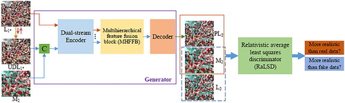
The fine-resolution image L₂ can be decomposed into a low-frequency coarse-resolution image and high-frequency details. The high-frequency details of the L_1* image are used to predict the high-frequency details of the PL₂ image. The prior image M₂ contributes to providing the low-frequency coarse-resolution data. Furthermore, to reduce the sensor bias between the Landsat and MODIS images, the UDL ${}_{1*}$ image is introduced to provide prior information of the reference date. Consequently, the UDL ${}_{1*}$ image and M₂ image concatenated as inputs conduce to provide prior information and obtain low-frequency features.

The generator consists of a dual-stream encoder, an MHFFB and a decoder. First, the dual-stream encoder takes L ${}_{1*}$ and C(UDL ${}_{1*},$ M₂) as inputs to extract high-frequency details and low-frequency information, respectively. Second, the MHFFB fuses global multihierarchical details to derive final high-frequency details and fuses global multihierarchical low-frequency features to obtain final low-frequency information. Finally, the decoder reconstructs the extracted features to generate the predicted image PL₂. M₂ is taken as the condition forming an image pair M₂-PL₂ or M₂-L₂ as the input of the RaLSD, and the probability that the predicted image PL₂ is more realistic than the real image L₂ or that the real image L₂ is more realistic than the predicted image PL₂ is estimated.

3.2. Architecture of generator

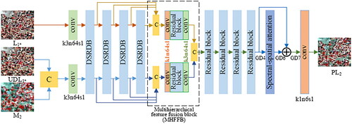
This subsection elaborates on the generator architecture of the EDRGAN-STF model, as illustrated in Figure 3. The generator contains a dual-stream encoder, an MHFFB and a decoder. Due to the great gap in spatial resolution between MODIS and Landsat images, i.e. the spatial resolution of MODIS and Landsat data used in this article is 500 m and 25 m and the ratio is 20, the low-resolution MODIS images express limited information, and only the low-frequency information extracted from MODIS images is not enough to express the low-frequency features in Landsat images. Moreover, there is a bias between Landsat and MODIS images due to different sensors and imaging conditions. Li et al. (2022a) validated that the spatial information of the downsampled Landsat image is closer to the Landsat image than the MODIS image, and it is more reasonable to restore the fine image using the downsampled Landsat image. Therefore, in this article, the UDL ${}_{1*}$ image degraded version of the L ${}_{1*}$ image is introduced as prior information to provide low-frequency information and improve the quality of the predicted image PL₂.

Figure 3. Generator architecture of EDRGAN-STF.

3.2.1. Dual-stream residual dense block

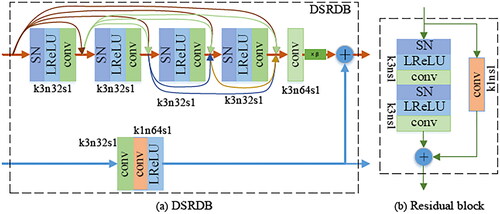
The dual-stream encoder is composed of one convolutional layer and four DSRDBs. One branch takes L ${}_{1*}$ as the input to extract dense high-frequency details, the other branch takes UDL ${}_{1*}$ and M₂ as the input to extract low-frequency information of the coarse image, and the two branches form a residual structure. The convolutional layer is used to extract shallow features, and DSRDBs are used to extract high-level features; the DSRDB structure is shown in Figure 4(a). Based on the observation of ESRGAN (Wang et al. 2019), more layers and connections can improve the network performance, and it is confirmed that the residual dense block (RDB) performs better than the conventional residual block (as shown in Figure 4(b)). Inspired by the above ideas, a DSRDB structure is proposed. The proposed DSRDB is a dual-stream residual-dense structure, which consists of dense connection layers, local feature fusion and local residual learning, forming a persistent memory mechanism. The upper branch with the dense structure is used to extract the high-frequency details of the reference image L ${}_{1*}.$ The convolutional structure employs the ‘switchable normalization (SN) (Luo et al. 2019) + Leaky ReLU (LReLU) (Nwankpa et al. 2021) + conv’ mode. SN unifies the instance normalization (IN), layer normalization (LN) and batch normalization (BN) (Luo et al. 2019). It is not necessary to manually design the normalization method of each layer. SN uses differentiable learning to determine the appropriate normalization operation. SN is a task- and data-driven method that motivates or suppresses the training effects for optimal results. The activation function LReLU can handle the neuron death problem and gradient direction jaggies (Nwankpa et al. 2021). In Figure 4(a), k3n32s1 indicates that the size of the convolution kernels is 3 × 3, the number is 32, and the stride is 1. The lower branch of the DSRDB is used to extract the low-frequency information of the prior images M₂ and UDL ${}_{1*}.$ The convolution kernel with the size of 3 × 3 is employed to extract low-frequency features, and the convolution kernel with the size of 1 × 1 is employed to adaptively change the number of the feature maps. The dual-stream information constitutes the residual structure, and the high-frequency details are multiplied by a constant β with a value ranging from 0 to 1 to shrink the residual and improve network stability (Wang et al. 2019).

Figure 4. DSRDB structure and residual block.

3.2.2. Multihierarchical feature fusion block

To take full advantage of the multilevel features extracted by DSRDBs, the different-level features are forwarded to the end of the encoder and fused. The MHFFB comprises two branches, displayed in Figure 3, the upper branch is designed to fuse global multihierarchical high-frequency features to derive final high-frequency details and the bottom branch is used to fuse multihierarchical low-frequency features to obtain final low-frequency information. The MHFFB consists of concatenation operations (i.e. C in Figure 3), convolutional layers (i.e. conv in Figure 3), and a residual block. The residual block adopts the conventional residual structure (He et al. 2016), as shown in Figure 4(b), where k3ns1 indicates that the size of the convolution kernels is 3 × 3, the number n is 64, and the stride is 1. The two branches have the same structure and do not share parameters. The four-level global features generated by the four DSRDBs are fed into the MHFFB. The four-level global high-frequency details are first concatenated and initially fused using a convolution operation followed by the LReLU to reduce the number of feature maps and improve the nonlinear fitting ability of the model. Then the generated features are further fused by a residual block and a convolution operation. The fusion procedure of four-level global low-frequency information is the same as that of the four-level global high-frequency details. Finally, the final fusion results are concatenated and transmitted to the decoder.

3.2.3. Decoder with spectral-spatial attention

The decoder consists of four residual blocks, a spectral-spatial attention block (SSAB) and a convolutional layer. The residual block is shown in Figure 4(b), the numbers of convolution kernels are 128, 64, 32 and 16, and the stride is 1. The residual blocks reconstruct high-frequency details and low-frequency features. In addition, RSIs contain rich information, such as rivers, crops, vegetation, land and so on. However, various spectral bands and spatial locations contain information of different importance, which contributes differently to STF. A spectral-spatial attention mechanism is designed to focus on important spectral bands and spatial features and enhance the reconstruction of critical regions, thereby improving the prediction of phenological changes and land-cover-type changes. The specific implementation of the SSAB is shown in Figure 5. Let GD4 indicate the reconstructed feature map. First, the GD4 (the $H\times W\times C$ is $256\times 256\times 16$) is fed into the spectral attention block to obtain a spectral attention vector with a size of $1\times 1\times 16.$ The vector is multiplied by GD4 to obtain a modified feature map GD5 ($256\times 256\times 16$) with channel weights, which enhances GD4 through different spectral channels. Then, the GD5 is fed into the spatial attention block to obtain a spatial attention map with a size of $256\times 256\times 1.$ The map is multiplied with GD5 to obtain the modified feature GD6 ($256\times 256\times 16$), which strengthens GD5 through various spatial locations.

Figure 5. Spectral-spatial attention block (SSAB).

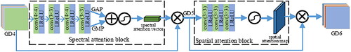
As shown in Figure 5, the spectral attention block consists of four convolutional layers followed by the LReLU. The two convolutional layers consist of 4 × 4 kernels with a stride of 4, and two convolutional layers comprise 3 × 3 kernels with a stride of 1, which gradually aggregates the spatial information. Then, the features are squeezed into two vectors using global average pooling (GAP) and global max pooling (GMP), respectively, an elementwise addition is applied and the following sigmoid function is employed to scale the value to [0, 1]. Finally, the spectral attention vector is multiplied with GD4 to enhance the features over various spectral channels, which refines GD4 through various spectral channels and is conducive to decreasing spectral distortion. The implementation is expressed as Equations (1)(1) $$M_{\mathit{ape}}=f_{\mathit{ape}}\left(G{D}_4;{\theta }_{\mathit{ape}}\right)$$(1) and (2)(2) $$G{D}_5=M_{\mathit{ape}}°G{D}_4$$(2) . (1) $$M_{\mathit{ape}}=f_{\mathit{ape}}\left(G{D}_4;{\theta }_{\mathit{ape}}\right)$$(1) (2) $$G{D}_5=M_{\mathit{ape}}°G{D}_4$$(2) where M_ape denotes the obtained spectral attention vector, $f_{\mathit{ape}}()$ and θ_ape indicate the function and parameter of the spectral attention block, GD₄ represents the input feature, GD₅ represents the reinforced feature, and $°$ means the elementwise multiplication.

The details of the spatial attention block are shown in Figure 5. The spatial attention module takes GD5 as input and consists of three convolutions with a kernel of 3 × 3, a stride of 1, and numbers of 8, 4 and 1. Each of them is followed by the LReLU. Finally, the sigmoid function is employed to generate a spatial attention map with values of [0, 1]. The map is multiplied with GD5 to obtain the refined feature map GD6, which enhances features in GD5 through various spatial locations and is conducive to decreasing spatial distortion. The procedures are expressed as Equations (3)(3) $$M_{\mathit{apa}}=f_{\mathit{apa}}\left(G{D}_5;{\theta }_{\mathit{apa}}\right)$$(3) and (4)(4) $$G{D}_6=M_{\mathit{apa}}°G{D}_5$$(4) . (3) $$M_{\mathit{apa}}=f_{\mathit{apa}}\left(G{D}_5;{\theta }_{\mathit{apa}}\right)$$(3) (4) $$G{D}_6=M_{\mathit{apa}}°G{D}_5$$(4) where M_apa denotes the obtained spatial attention map, $f_{\mathit{apa}}()$ and θ_apa indicate the function and parameter of the spatial attention block, and GD₆ represents the refined feature.

The refined feature map GD6 is generated by the SSAB, and GD6 and GD4 are added by a skip connection to obtain a feature map GD7, as shown in Figure 3, forming a residual structure. The spectral attention block can emphasize spectral bands that can aid in feature representation and STF, and establish correlations between spectral bands. The spatial attention block can enhance the same type of spatial information around the central pixel and suppress those with a different type. Finally, the GD7 is fed into the last reconstruction layer to generate the predicted image PL₂.

The expression of the generator of the proposed EDRGAN-STF model is Equation (5)(5) $$P{L}_2=G_{\vartheta }^{\mathit{EDRGAN}-\mathit{STF}}\left(L_{1^{*}},UD{L}_{1^{*}},M_2;\vartheta \right)$$(5) . (5) $$P{L}_2=G_{\vartheta }^{\mathit{EDRGAN}-\mathit{STF}}\left(L_{1^{*}},UD{L}_{1^{*}},M_2;\vartheta \right)$$(5) where PL₂ represents the Landsat image at prediction time t₂ generated by the EDRGAN-STF model. $G_{\vartheta }^{\mathit{EDRGAN}-\mathit{STF}}(·)$ represents the function of the generator of the EDRGAN-STF model, and the parameter is ϑ. L ${}_{1*}$ represents a reference Landsat image at an arbitrary time t₁, i.e. ARLI. UDL ${}_{1*}$ indicates the image obtained by downsampling and upsampling operations on the L ${}_{1*},$ i.e. DARLI. M₂ is the MODIS image at prediction time t₂ ($t_1\ne t_2$), i.e. PMI.

3.3. Architecture of RaLSD

The SGAN discriminator is used to predict whether the input image is real or generated, and the RaGAN discriminator predicts the probability that the real image is more realistic than the generated image, on average (Jolicoeur-Martineau 2019). The LSGAN solves the vanishing gradient problem caused by the SGAN (Mao et al. 2017). Considering the advantages of the RaGAN and LSGAN, the discriminator architecture is designed based on RaGAN and LSGAN, i.e. RaLSD, to improve the STF performance, as shown in Figure 6.

Figure 6. Network architecture of RaLSD.

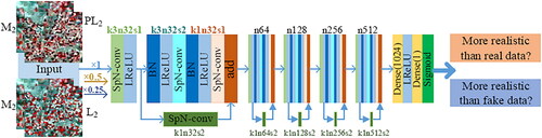
In Figure 6, the inputs of the RaLSD are the positive image pair M₂-L₂ or negative image pair M₂-PL₂, and M₂ is used as a condition to guide the network training. The RaLSD consists of five feature extraction blocks and two dense layers. The feature extraction block is composed of a plain convolution layer (i.e. a convolution operation and an LReLU function) and a residual block to enhance the expression ability of the network. The residual block reduces the image size while extracting features. k3n32s2 means that the convolution kernel size is 3 × 3, the number is 32 and the stride is 2. SpN-conv indicates that the SpN operation is performed on the convolution layer to improve the stability of the discriminator (Miyato et al. 2018). n64 indicates that the number of convolution kernels is 64, and the size and stride of the convolution kernels are the same as those in the first block. The dense layer is used to further reduce the dimension of feature maps. Moreover, a three-scale discriminator employed in the GAN-STFM (Tan et al. 2022) is used in RaLSD to improve the predicted image quality. The RaLSD inputs are downsampled to two scales with factors of 0.5 and 0.25, and three discriminators are trained with three-scale inputs and the same architecture as the RaLSD.

The expressions of the RaLSD are Equations (6)(6) $$D^{\mathit{RaLS}}\left(I_r,I_f\right)=\sigma \left(C\left(I_r\right)-{\mathbb{E}}_{I_f\sim \mathcal{Q}}\left[C\left(I_f\right)\right]\right)$$(6) and (7)(7) $$D^{\mathit{RaLS}}\left(I_f,I_r\right)=\sigma \left(C\left(I_f\right)-{\mathbb{E}}_{I_r\sim \mathcal{P}}\left[C\left(I_r\right)\right]\right)$$(7) . (6) $$D^{\mathit{RaLS}}\left(I_r,I_f\right)=\sigma \left(C\left(I_r\right)-{\mathbb{E}}_{I_f\sim \mathcal{Q}}\left[C\left(I_f\right)\right]\right)$$(6) (7) $$D^{\mathit{RaLS}}\left(I_f,I_r\right)=\sigma \left(C\left(I_f\right)-{\mathbb{E}}_{I_r\sim \mathcal{P}}\left[C\left(I_r\right)\right]\right)$$(7) where $D^{\mathit{RaLS}}(·)$ represents the relative probability estimated by the RaLSD, σ indicates the sigmoid function, $C(·)$ denotes the output of the non-transformed RaLSD, $\mathcal{P}$ is the distribution of the real data I_r, $\mathcal{Q}$ represents the distribution of the predicted data I_f, ${\mathbb{E}}_{I_r\sim \mathcal{P}}$ and ${\mathbb{E}}_{I_f\sim \mathcal{Q}}$ represent the expectations for all the real and predicted data in the batch.

3.4. Composite loss function

The composite losses of the EDRGAN-STF model consist of content losses of image and adversarial losses. The content losses ${\mathcal{L}}_{\mathit{content}}$ are the differences between the generated image and the GT image, including mean square error (MSE) of content, structural difference, feature loss and spectral difference.

MSE is a loss function that is widely used for optimization objectives, and the expression is shown in Equation (8)(8) $${\mathcal{L}}_{\mathit{MSE}}=\frac{1}{N}\sum _{i=1}^N{\left(L_2-P{L}_2\right)}^2$$(8) . (8) $${\mathcal{L}}_{\mathit{MSE}}=\frac{1}{N}\sum _{i=1}^N{\left(L_2-P{L}_2\right)}^2$$(8) where ${\mathcal{L}}_{\mathit{MSE}}$ represents the loss function of MSE, N is the batch size and L₂ represents the GT image of the predicted date.

The structural difference expresses the high-frequency detail difference between the generated image and the GT image, and the multiscale structural similarity (MS-SSIM) can effectively preserve the high-frequency details of the image (Zhao et al. 2017). The structural loss is expressed as Equation (9)(9) $${\mathcal{L}}_{MS-\mathit{SSIM}}=1-\mathit{SSI}{M}_{MS}\left(L_2,P{L}_2\right)\mathrm{ }=1-l_M\left(L_2,P{L}_2\right)·\prod _{k=1}^M{c}_k\left(L_2,P{L}_2\right)·s_k\left(L_2,P{L}_2\right)\mathrm{ }$$(9) (Wang et al. 2003) and the expression of SSIM is Equation (10)(10) $$\mathrm{SSIM}\left(L_2,P{L}_2\right)\mathrm{ }=l\left(L_2,P{L}_2\right)·c\left(L_2,P{L}_2\right)·s\left(L_2,P{L}_2\right)\mathrm{ }=\frac{\left(2{\mu }_{L_2}{\mu }_{P{L}_2}+b_1\right)\left(2{\sigma }_{L_{2}P{L}_2}+b_2\right)}{\left({\mu }_{L_2}{}^2+{\mu }_{P{L}_2}{}^2+b_1\right)\left({\sigma }_{L_2}^2+{\sigma }_{P{L}_2}^2+b_2\right)}\mathrm{ }$$(10) . (9) $${\mathcal{L}}_{MS-\mathit{SSIM}}=1-\mathit{SSI}{M}_{MS}\left(L_2,P{L}_2\right)\mathrm{ }=1-l_M\left(L_2,P{L}_2\right)·\prod _{k=1}^M{c}_k\left(L_2,P{L}_2\right)·s_k\left(L_2,P{L}_2\right)\mathrm{ }$$(9) (10) $$\mathrm{SSIM}\left(L_2,P{L}_2\right)\mathrm{ }=l\left(L_2,P{L}_2\right)·c\left(L_2,P{L}_2\right)·s\left(L_2,P{L}_2\right)\mathrm{ }=\frac{\left(2{\mu }_{L_2}{\mu }_{P{L}_2}+b_1\right)\left(2{\sigma }_{L_{2}P{L}_2}+b_2\right)}{\left({\mu }_{L_2}{}^2+{\mu }_{P{L}_2}{}^2+b_1\right)\left({\sigma }_{L_2}^2+{\sigma }_{P{L}_2}^2+b_2\right)}\mathrm{ }$$(10) where ${\mathcal{L}}_{MS-\mathit{SSIM}}$ is the loss function of the MS-SSIM. l_M, c_k and s_k are the M and k scale of the luminance l, contrast c and structure s defined in Equation (10)(10) $$\mathrm{SSIM}\left(L_2,P{L}_2\right)\mathrm{ }=l\left(L_2,P{L}_2\right)·c\left(L_2,P{L}_2\right)·s\left(L_2,P{L}_2\right)\mathrm{ }=\frac{\left(2{\mu }_{L_2}{\mu }_{P{L}_2}+b_1\right)\left(2{\sigma }_{L_{2}P{L}_2}+b_2\right)}{\left({\mu }_{L_2}{}^2+{\mu }_{P{L}_2}{}^2+b_1\right)\left({\sigma }_{L_2}^2+{\sigma }_{P{L}_2}^2+b_2\right)}\mathrm{ }$$(10) . ${\mu }_{L_2}$ and ${\mu }_{P{L}_2}$ denote the mean of images L₂ and PL₂, respectively. ${\sigma }_{L_{2}P{L}_2}$ represents the covariance between images L₂ and PL₂. ${\sigma }_{L_2}$ and ${\sigma }_{P{L}_2}$ represent the variance of images L₂ and PL₂, respectively. b₁ and b₂ are constants to avoid zeros in the denominator.

Feature loss is the perceptual similarity loss built on the feature layer of the pretrained network. According to ESRGAN (Wang et al. 2019), the distance between the two features before the activation function is minimized. The feature loss ${\mathcal{L}}_F$ is expressed as Equation (11)(11) $${\mathcal{L}}_F=\frac{1}{N}\sum _{i=1}^N{\left(\phi \left(L_2\right)-\phi \left(P{L}_2\right)\right)}^2$$(11) . (11) $${\mathcal{L}}_F=\frac{1}{N}\sum _{i=1}^N{\left(\phi \left(L_2\right)-\phi \left(P{L}_2\right)\right)}^2$$(11) where $\phi (L_2)$ and $\phi (P{L}_2)$ denote the feature maps of the pretrained model VGG-19 (Simonyan and Zisserman 2015) of images L₂ and PL₂, respectively.

The spectral difference can be represented by the spectral angle loss, i.e. the cosine similarity of the spectral vector between the generated image and GT image. The spectral loss function ${\mathcal{L}}_{\mathit{Spe}}$ is formulated as Equation (12)(12) $${\mathcal{L}}_{\mathit{Spe}}=1-\frac{\phi \left(L_2\right)·\phi \left(P{L}_2\right)}{\Vert \phi \left(L_2\right)\Vert \Vert \phi \left(P{L}_2\right)\Vert }$$(12) . (12) $${\mathcal{L}}_{\mathit{Spe}}=1-\frac{\phi \left(L_2\right)·\phi \left(P{L}_2\right)}{\Vert \phi \left(L_2\right)\Vert \Vert \phi \left(P{L}_2\right)\Vert }$$(12) where $\Vert ·\Vert$ represents the norm of the vector.

Adversarial losses are defined using the relativistic average least squares (RaLS) loss function (Baby and Verhulst 2019; Jolicoeur-Martineau 2019). The expression of the RaLSD loss function, i.e. ${\mathcal{L}}_D^{\mathit{RaLS}},$ is shown in Equation (13)(13) $${\mathcal{L}}_D^{\mathit{RaLS}}\mathrm{ }={\mathbb{E}}_{I_r\sim \mathcal{P}}\left[{\left(C\left(I_r\right)-{\mathbb{E}}_{I_f\sim \mathcal{Q}}\left[C\left(I_f\right)\right]-1\right)}^2\right]\mathrm{ }+{\mathbb{E}}_{I_f\sim \mathcal{Q}}\left[{\left(C\left(I_f\right)-{\mathbb{E}}_{I_r\sim \mathcal{P}}\left[C\left(I_r\right)\right]+1\right)}^2\right]\mathrm{ }$$(13) . (13) $${\mathcal{L}}_D^{\mathit{RaLS}}\mathrm{ }={\mathbb{E}}_{I_r\sim \mathcal{P}}\left[{\left(C\left(I_r\right)-{\mathbb{E}}_{I_f\sim \mathcal{Q}}\left[C\left(I_f\right)\right]-1\right)}^2\right]\mathrm{ }+{\mathbb{E}}_{I_f\sim \mathcal{Q}}\left[{\left(C\left(I_f\right)-{\mathbb{E}}_{I_r\sim \mathcal{P}}\left[C\left(I_r\right)\right]+1\right)}^2\right]\mathrm{ }$$(13)

The RaLS loss function of the generator, i.e. ${\mathcal{L}}_G^{\mathit{RaLS}},$ is expressed as Equation (14)(14) $${\mathcal{L}}_G^{\mathit{RaLS}}\mathrm{ }={\mathbb{E}}_{I_r\sim \mathcal{P}}\left[{\left(C\left(I_r\right)-{\mathbb{E}}_{I_f\sim \mathcal{Q}}\left[C\left(I_f\right)\right]+1\right)}^2\right]\mathrm{ }+{\mathbb{E}}_{I_f\sim \mathcal{Q}}\left[{\left(C\left(I_f\right)-{\mathbb{E}}_{I_r\sim \mathcal{P}}\left[C\left(I_r\right)\right]-1\right)}^2\right]\mathrm{ }$$(14) . (14) $${\mathcal{L}}_G^{\mathit{RaLS}}\mathrm{ }={\mathbb{E}}_{I_r\sim \mathcal{P}}\left[{\left(C\left(I_r\right)-{\mathbb{E}}_{I_f\sim \mathcal{Q}}\left[C\left(I_f\right)\right]+1\right)}^2\right]\mathrm{ }+{\mathbb{E}}_{I_f\sim \mathcal{Q}}\left[{\left(C\left(I_f\right)-{\mathbb{E}}_{I_r\sim \mathcal{P}}\left[C\left(I_r\right)\right]-1\right)}^2\right]\mathrm{ }$$(14)

The total losses of the generator of the proposed EDRGAN-STF model are expressed as Equation (15)(15) $${\mathcal{L}}_G\mathrm{ }={\mathcal{L}}_{\mathit{content}}+{\mathcal{L}}_G^{\mathit{RaLS}}\mathrm{ }=\alpha {\mathcal{L}}_{\mathit{MSE}}+\beta {\mathcal{L}}_{MS-\mathit{SSIM}}+\lambda {\mathcal{L}}_F+\gamma {\mathcal{L}}_{\mathit{Spe}}+\eta {\mathcal{L}}_G^{\mathit{RaLS}}\mathrm{ }$$(15) . (15) $${\mathcal{L}}_G\mathrm{ }={\mathcal{L}}_{\mathit{content}}+{\mathcal{L}}_G^{\mathit{RaLS}}\mathrm{ }=\alpha {\mathcal{L}}_{\mathit{MSE}}+\beta {\mathcal{L}}_{MS-\mathit{SSIM}}+\lambda {\mathcal{L}}_F+\gamma {\mathcal{L}}_{\mathit{Spe}}+\eta {\mathcal{L}}_G^{\mathit{RaLS}}\mathrm{ }$$(15) where ${\mathcal{L}}_G$ is the function of the composite losses, and $\alpha ,\beta ,\lambda ,\gamma$ and η are the weight coefficients.

4. Experiments

4.1. Data sets

The experiments employ two widely used data sets: cooperatively irrigation area (CIA) and lower gwydir catchment (LGC) (Emelyanova et al. 2013). The CIA lies in southern New South Wales, Australia, and covers a zone of 2193 km². The CIA data set contained 17 cloud-free Landsat-MODIS image pairs from 2001 to 2002. The Landsat products were received by the Landsat-7 ETM+. The MODIS data were the MODIS Terra MOD09GA Collection 5 product. The size of images is 1720 × 2040 with 6-band. The CIA area is spatially heterogeneous, including many scattered and irregular small-scale croplands. The CIA area contains abundant seasonal phenological changes and slight land-cover-type changes.

The LGC lies in northern New South Wales, Australia, and covers an area of 5440 km². The LGC data set contained 14 cloud-free Landsat-MODIS image pairs from 2004 to 2005. The Landsat products were obtained by the Landsat-5 TM. The MODIS data were the MODIS Terra MOD09GA Collection 5 product. The size of images is 3200 × 2720 with 6-band. The LGC area contains abundant land-cover-type changes.

The MODIS images have been stacked in the order of the Landsat bands, and the Landsat-MODIS image pairs have been co-registered with the resolution of 25 m. Because the CIA and LGC data were calibrated (Emelyanova et al. 2013), the edges of images appeared in some areas where there is no ground surface feature and the pixels are 0, denoted as valid data. These invalid data may affect the accuracy of traditional approaches and have no influence on DL-based models (Ma et al. 2021). To ensure the fairness of the comparison, the images are cropped to remove the invalid data. The size of CIA images is 1358 × 2032 × 6 and the size of LGC images is 3184 × 2708 × 6.

The data used consists of three images, including a Landsat image at an arbitrary date and a Landsat-MODIS image pair at the prediction date. The inputs for the network consist of a Landsat image at an arbitrary date and a MODIS image at the prediction date, and the Landsat image at the prediction date is employed as the GT. For the CIA data set, the training data set consists of the 1st–3rd and 10th–17th image pairs, where two pair of images in the training data set are randomly selected for validation. The 5th–9th image pairs are used as the testing data to be predicted. For the LGC data set, the training data set is composed of the 1st–6th and 12th–14th image pairs, where two pair of images in the training data set are randomly selected for validation. The 8th–11th image pairs are used as the testing data to be predicted.

4.2. Evaluation indicators

To evaluate the designed EDRGAN-STF model, the STF performance is estimated from subjective aspects and objective indicators according to the fused result and the GT image. For objective indicators, root mean square error (RMSE), spectral angle mapper (SAM) (Yuhas et al. 1992), structural similarity (SSIM) (Wang et al. 2003), erreur relative global adimensionnelle de synthése (ERGAS) (Vivone et al. 2021; Wu et al. 2022) and correlation coefficient (CC) (Li et al. 2020a) are employed. RMSE means the root mean square error between the predicted data and GT. The ideal value is 0, and the smaller the value, the better the prediction effect. SAM expresses the angle between the spectral vectors of the predicted and GT images, which belongs to an error index, denoting the spectral distortion of the predicted image. The ideal value is 0. The smaller the value of SAM, the less the spectral distortion of the fused image. SSIM represents the similarity of the structural details between the prediction and GT. The ideal value is 1. The closer SSIM is to 1, the more structural details are preserved in the predicted image and the less spatial distortion is. ERGAS is a comprehensive indicator that indicates the overall fusion quality of the predicted image. The ideal value is 0. The closer the value of ERGAS is to 0, the better the fusion result. CC denotes the linear relationship between the predicted data and GT and the ideal value is 1.

4.3. Experimental setup

The implementation framework of the model based on DL is PyTorch, and the STARFM and FSDAF models are implemented in IDL. The workstation includes two NVIDIA Tesla V100 PCIe GPUs with 16 GiB of video memory and an Intel Xeon CPU. The patch size of images for training is 256 × 256, the batch size is 16, and the epoch is 300. Set the weights of the total losses according to the SRGAN (Ledig et al. 2017) work, i.e. $\alpha =\beta =\lambda =\gamma =1$ and $\eta =1\times {10}^{-3}.$ The Adam (Kingma and Ba 2015) is employed to optimize the objective, with an initial learning rate of 0.0002. The number of input and output channels of the network is 6, which can be set as needed. The network is trained and tested simultaneously using 6-band. The training and testing of the DL models are done on the GPU, and the STARFM and FSDAF experiments are done on the CPU.

4.4. Experimental results and analysis

To better evaluate the STF model proposed in this article, four state-of-the-art comparative experiments are conducted on CIA and LGC data. Traditional methods include the weight-based fusion method STARFM (Gao et al. 2006) and the hybrid fusion method FSDAF (Zhu et al. 2016). DL-based methods include the EDCSTFN (Tan et al. 2019) and GAN-STFM (Tan et al. 2022) models. The inputs of the STARFM, FSDAF and EDCSTFN models are all three observed images, including a pair of Landsat-MODIS images of the reference date and a MODIS image of the predicted date. The inputs of the GAN-STFM are two observed images, including a Landsat image of the reference date and a MODIS image of the predicted date.

4.4.1. Experiments on CIA data

Table 1 demonstrates the quantitative indicators of each comparative method on the five groups of testing data from the CIA data set with spatial heterogeneity. The RMSE, SSIM and CC indicators are the average of each band, while the SAM and ERGAS indicators are calculated using 6-band. The bold numbers indicate that the fusion result is the best. The metrics in Table 1 show that the designed EDRGAN-STF technique is the best in terms of radiation fidelity, structure preservation and spectral fidelity compared with the STARFM, FSDAF, EDCSTFN and GAN-STFM techniques. It can also be found that the STARFM, FSDAF, EDCSTFN and GAN-STFM methods have different prediction performances on the five groups of data. For example, the FSDAF performs better on the 1st and 4th data and the GAN-STFM performs better on the 3th and 5th data. Moreover, the proposed EDRGAN-STF method has the best prediction performance on the five groups of data, and the robustness is good.

Table 1. Quantified indicators of comparative methods on the five groups of testing data of the CIA dataset with spatial heterogeneity.

Predicted date	Model	RMSE	SSIM	ERGAS	SAM	CC
20011125	STARFM	0.0296	0.8371	0.9874	0.1030	0.8131
	FSDAF	0.0292	0.8375	0.9627	0.1072	0.8157
	EDCSTFN	0.0293	0.8333	0.9537	0.1096	0.8223
	GAN-STFM	0.0314	0.8212	1.0309	0.1181	0.8021
	EDRGAN-STF	0.0269	0.8522	0.8936	0.1003	0.8632
20011204	STARFM	0.0294	0.8712	0.9137	0.0861	0.8639
	FSDAF	0.0292	0.8591	0.8314	0.0890	0.8508
	EDCSTFN	0.0305	0.8679	1.0294	0.0858	0.8620
	GAN-STFM	0.0316	0.8415	0.9281	0.0973	0.8212
	EDRGAN-STF	0.0292	0.8840	0.8235	0.0849	0.8779
20020105	STARFM	0.0380	0.8267	0.9689	0.1181	0.8084
	FSDAF	0.0375	0.8437	0.9969	0.0858	0.8403
	EDCSTFN	0.0368	0.8443	1.0083	0.0981	0.8309
	GAN-STFM	0.0355	0.8133	0.9283	0.0838	0.8220
	EDRGAN-STF	0.0326	0.8515	0.8547	0.0764	0.8570
20020112	STARFM	0.0292	0.8803	0.7928	0.0827	0.9345
	FSDAF	0.0235	0.8955	0.7236	0.0700	0.9354
	EDCSTFN	0.0374	0.8730	0.9029	0.0754	0.9215
	GAN-STFM	0.0279	0.8557	0.7833	0.0762	0.8935
	EDRGAN-STF	0.0224	0.9070	0.6254	0.0635	0.9398
20020213	STARFM	0.0318	0.8226	1.0362	0.0988	0.8537
	FSDAF	0.0320	0.8389	1.0094	0.1118	0.8608
	EDCSTFN	0.0315	0.8606	0.9363	0.0919	0.8681
	GAN-STFM	0.0255	0.8616	0.8133	0.0770	0.8989
	EDRGAN-STF	0.0225	0.8904	0.6956	0.0603	0.9275

The fusion results for CIA data are elaborated. From January to February 2002, crops in irrigated cropland grew rapidly and the phenology changed greatly, while the surrounding woodlands and rivers did not change much, making the CIA region spatially heterogeneous. Consequently, the Landsat-MODIS image pair on January 12, 2002, is selected as the prior data (the GAN-STFM and proposed EDRGAN-STF methods only use the Landsat image), and the predicted date is February 13, 2002. The predicted results of the compared methods for the CIA data on February 13, 2002, are shown in Figure 7. The near infrared-red-green band is employed as the R-G-B channel to better display the characteristics of crops. Figure 7(a) is a captured Landsat image on January 12, 2002, Figure 7(b,c) is the captured MODIS image and Landsat image on February 13, 2002, and Figure 7(d–h) is the predicted images obtained by the STARFM, FSDAF, EDCSTFN, GAN-STFM and EDRGAN-STF methods, respectively. To better compare the predicted results of the various methods, contents in the yellow rectangle in Figure 7 are enlarged and the enlarged details are displayed in Figure 8. Figure 8(a,b) is the enlarged details of MODIS and Landsat images on the predicted date. Figure 8(c–g) is the enlarged details of the predicted results of the STARFM, FSDAF, EDCSTFN, GAN-STFM and EDRGAN-STF, respectively. Absolute error maps (AEMs) between the predictions and the GT image are used to more conveniently observe the differences of fusion results, as shown in Figure 9. AEM is displayed in colour, and the colour bar from blue to red indicates that the error is increasing from 0 to 1.

Figure 7. Predicted results of the compared methods for the CIA data on February 13, 2002. (a) Observed Landsat image on January 12, 2002. (b) Observed MODIS image on February 13, 2002. (c) Observed Landsat image on February 13, 2002, i.e. Ground Truth . (d) STARFM. (e) FSDAF. (f) EDCSTFN. (g) GAN-STFM. (h) EDRGAN-STF.

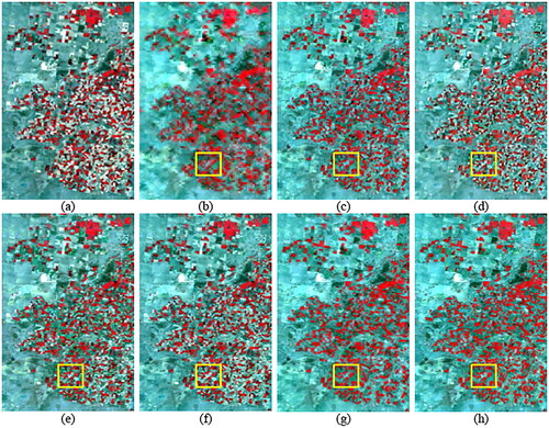
Figure 8. Enlarged details in the yellow rectangle in Figure 7. (a) Observed MODIS image on February 13, 2002. (b) Ground Truth . (c) STARFM. (d) FSDAF. (e) EDCSTFN. (f) GAN-STFM. (g) EDRGAN-STF.

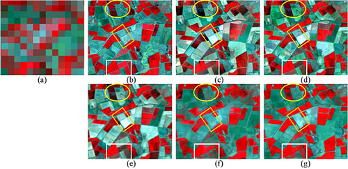
Figure 9. Absolute error maps between the predictions and GT of the CIA data on February 13, 2002. (a) STARFM. (b) FSDAF. (c) EDCSTFN. (d) GAN-STFM. (e) EDRGAN-STF.

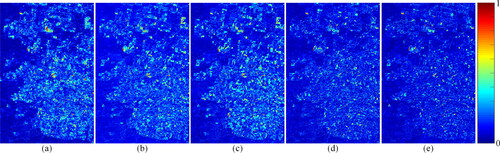
By visually comparing the fused results and GT of each method in Figure 7, it is clearly observed that the FSDAF, GAN-STFM and EDRGAN-STF methods can predict the phenological changes of cropland in some degree, but the ability of the STARFM and EDCSTFN to predict the phenological changes is poor. From Figure 9, it can also be clearly observed that the deviation between the fused results of the EDRGAN-STF and GT is the smallest. For spatially heterogeneous regions, the enlarged details of the fused results of each method are significantly different. It can be clearly found that the result of the proposed EDRGAN-STF model is closer to Figure 8(b). For the contents in the yellow ellipse in Figure 8(b), the details of the EDRGAN-STF are closer, while the content and spectral losses of the STARFM, FSDAF, EDCSTFN and GAN-STFM are more serious. For the contents of the orange box in Figure 8(b), the STARFM, FSDAF and EDCSTFN suffer from severe loss of detail and colour, and the GAN-STFM blurs the edges. For the contents of the white box in Figure 8(b), the EDRGAN-STF has the best results, while the STARFM, FSDAF, EDCSTFN and GAN-STFM methods suffer from severe structural and spectral losses. These demonstrate that the EDRGAN-STF is more robust in predicting regions with spatial heterogeneity. From Table 1, we clearly find that the designed EDRGAN-STF model is the best on RMSE, SSIM, ERGAS, SAM and CC for the predicted data of the CIA on February 13, 2002.

4.4.2. Experiments on LGC data

Table 2 presents the quantified evaluation indices of the comparative methods on the LGC data set with slight phenological and extensive land-cover-type changes. It is evidently observed that the proposed EDRGAN-STF displays the best on RMSE, SSIM, ERGAS, SAM and CC for the predicted results of the four groups of testing data. The prediction performance of the FSDAF is better than that of the GAN-STFM for the first testing data with drastic land-cover-type changes, and the prediction ability of the GAN-STFM is better than that of the FSDAF on the other three testing data. The prediction ability of the STARFM and EDCSTFN on the four groups of testing data is also different. The proposed EDRGAN-STF method has the best prediction ability and stable performance on the four groups of testing data, and the robustness is better.

Table 2. Quantified indices of the comparative methods on the LGC data having extensive land-cover-type changes.

Predicted date	Model	RMSE	SSIM	ERGAS	SAM	CC
20041212	STARFM	0.0586	0.6964	3.7740	0.3812	0.2118
	FSDAF	0.0349	0.7720	2.2670	0.2070	0.7413
	EDCSTFN	0.0504	0.7531	1.8519	0.2768	0.6436
	GAN-STFM	0.0376	0.7456	1.8014	0.2294	0.6999
	EDRGAN-STF	0.0347	0.7769	1.6336	0.1894	0.7434
20041228	STARFM	0.0337	0.8069	1.4473	0.1504	0.7761
	FSDAF	0.0324	0.7987	1.3933	0.1396	0.7796
	EDCSTFN	0.0408	0.8060	1.7202	0.1917	0.6365
	GAN-STFM	0.0287	0.8335	1.1537	0.1252	0.8136
	EDRGAN-STF	0.0259	0.8554	1.0477	0.1107	0.8475
20050113	STARFM	0.0232	0.8921	0.7964	0.0842	0.8738
	FSDAF	0.0217	0.8879	0.7509	0.0811	0.8815
	EDCSTFN	0.0224	0.9014	0.8081	0.0813	0.8618
	GAN-STFM	0.0202	0.9160	0.6592	0.0669	0.9065
	EDRGAN-STF	0.0178	0.9289	0.5943	0.0618	0.9213
20050129	STARFM	0.0252	0.8943	0.8832	0.0776	0.8975
	FSDAF	0.0253	0.8825	0.8888	0.0744	0.8956
	EDCSTFN	0.0280	0.8834	1.0040	0.0892	0.8545
	GAN-STFM	0.0232	0.8946	0.7975	0.0707	0.8954
	EDRGAN-STF	0.0222	0.9012	0.7666	0.0677	0.9068

A large flood happened in December 2004, bringing about abnormally abrupt land-cover-type changes. A group of testing data in LGC with abrupt land-cover-type changes is selected to elaborate on the fused results of the contrastive methods. Consequently, Landsat and MODIS images on November 26, 2004, are the prior data (the GAN-STFM and proposed EDRGAN-STF only use the Landsat image), and the date of the predicted image is December 12, 2004. The predicted data of the compared methods for the LGC data on December 12, 2004, are shown in Figure 10. Figure 10(a) is a captured Landsat image on November 26, 2004, Figure 10(b) is a captured MODIS image on December 12, 2004, Figure 10(c) is a captured Landsat image on December 12, 2004, i.e. GT, and Figure 10(d–h) is predicted images obtained by the STARFM, FSDAF, EDCSTFN, GAN-STFM and EDRGAN-STF methods, respectively. To better compare the predicted results of the various methods, contents in the yellow and orange rectangles in Figure 10 are enlarged and the enlarged details are displayed in Figure 11. In Figure 11, the up row is the enlarged contents in the yellow rectangle in Figure 10 and the second row is the enlarged details of the contents in the orange rectangle in Figure 10. Figure 10(a) is the enlarged details of the Landsat image on December 12, 2004. Figure 10(b–f) is the enlarged details of the predictions of the STARFM, FSDAF, EDCSTFN, GAN-STFM and EDRGAN-STF, respectively. The AEMs between the predictions and the GT image are displayed in Figure 12.

Figure 10. Predicted data of the compared models for the LGC data on December 12, 2004. (a) Observed Landsat image on November 26, 2004. (b) Observed MODIS image on December 12, 2004. (c) Observed Landsat image on December 12, 2004, i.e. Ground Truth. (d) STARFM. (e) FSDAF. (f) EDCSTFN. (g) GAN-STFM. (h) EDRGAN-STF.

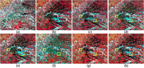
Figure 11. Enlarged details in the yellow and orange rectangles in Figure 10. (The top row is the enlarged view of the yellow rectangle in Figure 10, and the bottom row is the enlarged view of the orange box in Figure 10.) (a) Ground Truth. (b) STARFM. (c) FSDAF. (d) EDCSTFN. (e) GAN-STFM. (f) EDRGAN-STF.

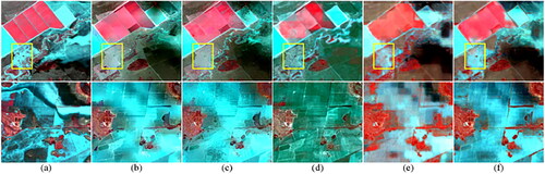
Figure 12. Absolute error maps between the predicted data and GT of the LGC data on December 12, 2004. (a) STARFM. (b) FSDAF. (c) EDCSTFN. (d) GAN-STFM. (e) EDRGAN-STF.

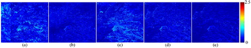
From Figure 10, it is obviously watched that the predicted result of the EDCSTFN method appears relatively severe colour distortion. Combined with Figure 12, it is observed that the absolute error between the predicted data of the STARFM and the GT image is large. The prediction of the proposed EDRGAN-STF is the closest to the GT image. From the yellow box area in the first row of Figure 11, it is evident that the flood-cover zone acquired by the EDRGAN-STF is the closest to the GT image, the STARFM and FSDAF fail to predict the flood-cover zone, and the flood-cover zone predicted by the EDCSTFN and GAN-STFM is quite different from that in GT image. In addition, from the red vegetation area, the STARFM, FSDAF and EDCSTF methods generate a lot of fake details, the predicted result of the FSDAF method suffers severe artifacts, and the predicted results of the STARFM and EDCSTFN appear severe spectral distortion. Compared with the GAN-STFM, the prediction of the designed EDRGAN-STF method is closer to the GT image. From the second row of Figure 11, it can be distinctly observed that the prediction of the designed EDRGAN-STF is the closest to the GT image in both spectral fidelity and structural fidelity. From Table 2, it is obvious that the EDRGAN-STF is optimal towards RMSE, SSIM, ERGAS, SAM and CC for the predicted data of the LGC on December 12, 2004. These illustrate the advantages of the EDRGAN-STF method in spectral preservation and prediction of significant land-cover-type changes.

4.4.3. Ablation experiments

To confirm the significance of the input UDL ${}_{1*},$ DSRDB, MHFFB, SSAB and RaLSD in the proposed EDRGAN-STF model, ablation experiments are conducted on the CIA and LGC testing data for the five blocks. The following are the five structures of the ablation experiments.

Validity of the input UDL ${}_{1*}:$ The UDL ${}_{1*}$ image is removed from the proposed EDRGAN-STF model, only L ${}_{1*}$ and M₂ data are employed, and other structures are consistent with the EDRGAN-STF, denoted as EDRGAN-STF-NDL.

Effectiveness of the DSRDB: DSRDBs are displaced by the residual blocks, and other structures are consistent with the EDRGAN-STF, denoted as EDRGAN-STF-NRDB.

Effectiveness of the MHFFB: The MHFFB in the EDRGAN-STF model is removed and the outputs of the encoder are directly fed into the decoder in the generator. The other structures are consistent with the EDRGAN-STF, denoted as EDRGAN-STF-NMF.

Validity of the SSAB: The SSAB in the EDRGAN-STF model is removed and other architectures are consistent with the EDRGAN-STF, labelled as EDRGAN-STF-NA.

Validity of the RaLSD: The RaLSD is replaced by a least squares discriminator and other architectures are consistent with the EDRGAN-STF model, marked as EDRGAN-STF-NRa.

The quantitative evaluation indicators of the experimental results on the CIA and LGC testing data are shown in Tables 3 and 4. From Tables 3 and 4, it is clearly discovered that the EDRGAN-STF attains the best fusion performance on both CIA data and LGC data combining the five indicators. The five blocks all play a positive role in improving the accuracy of STF, which proves the effectiveness of the five blocks in the STF of RSIs.

Table 3. Quantified indicators of the predicted data of ablation experiments on the CIA data.

Predicted date	Model	RMSE	SSIM	ERGAS	SAM	CC
20011125	EDRGAN-STF-NRDB	0.0290	0.8367	0.9545	0.1083	0.8362
	EDRGAN-STF-NDL	0.0288	0.8367	0.9396	0.1040	0.8372
	EDRGAN-STF-NMF	0.0301	0.8220	0.9700	0.1214	0.8212
	EDRGAN-STF-NA	0.0292	0.8340	0.9494	0.1108	0.8316
	EDRGAN-STF-NRa	0.0291	0.8401	0.9642	0.1107	0.8401
	EDRGAN-STF	0.0269	0.8522	0.8936	0.1003	0.8632
20020112	EDRGAN-STF-NRDB	0.0272	0.8609	0.7893	0.0691	0.8937
	EDRGAN-STF-NDL	0.0275	0.8819	0.7486	0.0676	0.9036
	EDRGAN-STF-NMF	0.0266	0.8804	0.7344	0.0720	0.8997
	EDRGAN-STF-NA	0.0272	0.8843	0.7710	0.0747	0.8939
	EDRGAN-STF-NRa	0.0292	0.8605	0.8063	0.0781	0.8934
	EDRGAN-STF	0.0224	0.9070	0.6254	0.0635	0.9398

Table 4. Quantified indicators of the predicted data of ablation experiments on the LGC data.

Predicted date	Model	RMSE	SSIM	ERGAS	SAM	CC
20041212	EDRGAN-STF-NRDB	0.0355	0.7562	1.7073	0.2055	0.6982
	EDRGAN-STF-NDL	0.0366	0.7614	1.6573	0.2053	0.7057
	EDRGAN-STF-NMF	0.0352	0.7605	1.7161	0.2121	0.7342
	EDRGAN-STF-NA	0.0356	0.7698	1.7107	0.1945	0.7340
	EDRGAN-STF-NRa	0.0362	0.7628	1.6697	0.2037	0.7317
	EDRGAN-STF	0.0347	0.7769	1.6336	0.1894	0.7434
20050129	EDRGAN-STF-NRDB	0.0238	0.8936	0.8509	0.0741	0.8984
	EDRGAN-STF-NDL	0.0238	0.8961	0.8927	0.0701	0.8957
	EDRGAN-STF-NMF	0.0229	0.8930	0.8034	0.0719	0.9035
	EDRGAN-STF-NA	0.0227	0.8968	0.8102	0.0684	0.9009
	EDRGAN-STF-NRa	0.0224	0.8988	0.7927	0.0681	0.9067
	EDRGAN-STF	0.0222	0.9012	0.7666	0.0677	0.9068

4.4.4. Computation and time

As displayed in Table 5, the EDCSTFN, GAN-STFM and EDRGAN-STF models are compared through three aspects: model parameters, floating point operations (FLOPs) and testing time. The STARFM and FSDAF models are compared through testing time. The unit G means 10⁹ and k is 10³. Table 5 exhibits the parameters and FLOPs of the generator of the GAN-STFM and EDRGAN-STF models. The testing time is obtained from the CIA data on November 25, 2001, with a size of 1358 × 2032 × 6. The EDCSTFN, GAN-STFM and EDRGAN-STF models are conducted on the aforementioned GPU, while the STARFM and FSDAF approaches are implemented on the aforementioned CPU. From Table 5, it is observed that the EDCSTFN has fewer parameters and FLOPs and takes the least time, and the EDRGAN-STF has more parameters, FLOPs and time than the GAN-STFM. This is because the EDRGAN-STF contains the dense connections, MHFFB, SSAB and the input UDL ${}_{1*}.$ However, the testing time of the EDRGAN-STF model is acceptable.

Table 5. Model complexity and testing time.

Model	Parameters (k)	FLOPs (G)	Testing time (s)
EDCSTFN	284.134	18.5850	0.3776
GAN-STFM	578.130	37.7597	0.5519
EDRGAN-STF	850.126	56.2697	1.3096
FSDAF	–	–	2425.0150
STARFM	–	–	1133.2600

5. Discussion

5.1. Effect of reference image

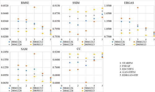
The selection of reference images is very important for the existing STF methods. At present, in addition to the GAN-STFM method, the date of the reference image of other STF methods is close to the predicted date. Impacts of reference images with different dates on the predicted results are analyzed. To observe the difference more conveniently, quantitative evaluation indicators are visualized in Figures 13 and 14, where 1–5 of the horizontal axis represent the STARFM, FSDAF, EDCSTFN, GAN-STFM and EDRGAN-STF methods, respectively, and colours indicate the predicted results using reference images with different dates. Figure 13 shows the quantified indicators of the predicted results of the CIA data on February 13, 2002, with the reference images on November 9, 2001, November 25, 2001, December 4, 2001, January 5, 2002 and January 12, 2002. Figure 14 shows the quantified indicators of the predicted results of the LGC data on January 29, 2005, with the reference images on November 26, 2004, December 12, 2004, December 28, 2004 and January 13, 2005. From Figures 13 and 14, it is discovered that the designed EDRGAN-STF method has the smallest difference under the influence of different reference images, followed by the GAN-STFM model, while the STARFM, FSDAF and EDCSTFN methods have great differences. In addition, the predicted results of the designed EDRGAN-STF model have the best performance.

Figure 13. Quantified indicators of the predicted data of the CIA on February 13, 2002, using reference images with different dates.

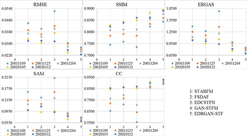
Figure 14. Quantified indicators of the predicted data of the LGC on January 29, 2005, using reference images with different dates.

5.2. Inputs of STF model

The majority of STF models require at least three observed images illustrated in Figure 1(a) and (b). Whereas, the GAN-STFM model requires a Landsat image of the reference date and a MODIS image of the predicted date. Due to the influence of natural factors such as weather, few high-quality image pairs can be used as the reference data and the previous subsection also proves that the STF accuracy is affected by the reference image. In addition, the DL-based STF model requires numerous high-quality image pairs as the training data. Therefore, the number of input images is also a considerable element affecting the practical application of the STF model. The proposed EDRGAN-STF model also needs a observed Landsat image with the reference time and a observed MODIS image with the predicted time. Although the input of the proposed EDRGAN-STF model also requires the down-resolution Landsat image, which does not need to be acquired by the sensor and can be achieved directly through the degraded-resolution operation. Without increasing the number of observed images, the STF accuracy is improved by introducing the reduced-resolution Landsat image and the EDRGAN-STF model is minimally affected by the reference image, which has great prospects in practical applications.

6. Conclusion

In this article, an enhanced STF model with degraded fine-resolution images via relativistic generative adversarial networks is proposed, i.e. EDRGAN-STF. The EDRGAN-STF model is an end-to-end network with all bands trained simultaneously. The inputs of the EDRGAN-STF only contain the ARLI, DARLI and PMI. The introduction of the DARLI reduces the bias caused by different sensors. The DSRDB and MHFFB of the generator more fully capture the local and global spatial details of ARLI and low-frequency information of DARLI and PMI. The spectral-spatial attention mechanism used in the decoder enhances the reconstruction of critical regions and improves the prediction of phenological changes and land-cover-type changes. A new composite loss function is introduced to better optimize the designed STF model. Comparative experiments are conducted employing four state-of-the-art methods on CIA and LGC data sets, ablation experiments are performed, and the experimental results are analyzed and discussed. Both objective and quantitative evaluations reveal that the EDRGAN-STF method improves the STF accuracy and has stronger robustness for different reference images, which has great prospects in practical applications. It is still a challenge for STF method to predict the sudden changes of irregular land-cover-type. In addition, the spatio-temporal-spectral integrated fusion (Peng et al. 2021) is difficulty to be solved in RSIs fusion. In the future, we will study to further improve the prediction precision and research spatio-temporal-spectral integrated fusion.

Disclosure statement

No potential conflict of interest was reported by the author(s).

Additional information

Funding

The work was supported by Hainan Major Science and Technology Program of China under Grant ZDKJ202017, Hainan Provincial Natural Science Foundation of China under Grant 2019CXTD400 and the National Key Research and Development Program of China under Grant 2018YFB1404400.

References

- Arjovsky M, Chintala S, Bottou L. 2017. Wasserstein generative adversarial networks. In: Proc. 34th Int. Conf. Mach. Learn.; vol. 70; Aug; Sydney, Australia. p. 214–223.
- Baby D, Verhulst S. 2019. Sergan: speech enhancement using relativistic generative adversarial networks with gradient penalty. In: Proc. 2019 IEEE Int. Conf. Acoust. Speech Signal Process. (ICASSP); May; Brighton, UK. p. 106–110.
- Benzenati T, Kessentini Y, Kallel A. 2022. Pansharpening approach via two-stream detail injection based on relativistic generative adversarial networks. Expert Syst Appl. 188:115996.
- Chen Y, Shi K, Ge Y, Zhou Y. 2022. Spatiotemporal remote sensing image fusion using multiscale two-stream convolutional neural networks. IEEE Trans Geosci Remote Sens. 60:1–12.
- Emelyanova IV, McVicar TR, Van Niel TG, Li LT, Van Dijk AI. 2013. Assessing the accuracy of blending Landsat–MODIS surface reflectances in two landscapes with contrasting spatial and temporal dynamics: a framework for algorithm selection. Remote Sens Environ. 133:193–209.
- Gao F, Masek J, Schwaller M, Hall F. 2006. On the blending of the Landsat and MODIS surface reflectance: predicting daily Landsat surface reflectance. IEEE Trans Geosci Remote Sens. 44(8):2207–2218.
- Gastineau A, Aujol JF, Berthoumieu Y, Germain C. 2022. Generative adversarial network for pansharpening with spectral and spatial discriminators. IEEE Trans Geosci Remote Sens. 60:1–11.
- Goodfellow I, Pouget-Abadie J, Mirza M, Xu B, Warde-Farley D, Ozair S, Courville A, Bengio Y. 2014. Generative adversarial nets. Adv Neural Inf Process Syst. 27:2672–2680.
- Guo D, Shi W, Hao M, Zhu X. 2020. FSDAF 2.0: improving the performance of retrieving land cover changes and preserving spatial details. Remote Sens Environ. 248:111973.
- Haut JM, Paoletti ME, Plaza J, Plaza A, Li J. 2019. Visual attention-driven hyperspectral image classification. IEEE Trans Geosci Remote Sens. 57(10):8065–8080.
- He KM, Zhang XY, Ren SQ, Sun J. 2016. Identity mappings in deep residual networks. In: 14th Eur. Conf. Comput. Vis. (ECCV). Lect. Notes Comput. Sci.; vol. 9908; Oct; Amsterdam, Netherlands. p. 630–645.
- Hou S, Sun W, Guo B, Li X, Zhang J, Xu C, Li X, Shao Y, Li C. 2022. RFSDAF: a new spatiotemporal fusion method robust to registration errors. IEEE Trans Geosci Remote Sens. 60:1–18.
- Hu J, Shen L, Albanie S, Sun G, Wu EH. 2020. Squeeze-and-excitation networks. IEEE Trans Pattern Anal Mach Intell. 42(8):2011–2023.
- Huang B, Song H. 2012. Spatiotemporal reflectance fusion via sparse representation. IEEE Trans Geosci Remote Sens. 50(10):3707–3716.
- Jang DW, Park RH. 2019. Densenet with deep residual channel-attention blocks for single image super resolution. In Proc. 32nd IEEE Comput. Soc. Conf. Comput. Vis. Pattern Recogn. Workshops; Jun; Long Beach, CA, USA. p. 1795–1803.
- Jolicoeur-Martineau A. 2019. The relativistic discriminator: a key element missing from standard GAN. In: 7th Int. Conf. Learn. Represent. (ICLR); May; New Orleans, LA, USA. p. 1–26.
- Kingma DP, Ba JL. 2015. Adam: a method for stochastic optimization. In: 3rd Int. Conf. Learn. Represent. (ICLR); May; San Diego, CA. p. 1–15.
- Ledig C, Theis L, Huszár F, Caballero J, Cunningham A, Acosta A, Aitken A, Tejani A, Totz J, Wang Z. 2017. Photo-realistic single image super-resolution using a generative adversarial network. In: Proc. 30th IEEE Conf. Comput. Vis. Pattern Recognit. (CVPR); Jul; Honolulu, HI, USA. p. 105–114.
- Li J, Huo H, Li C, Wang R, Feng Q. 2021a. AttentionFGAN: infrared and visible image fusion using attention-based generative adversarial networks. IEEE Trans Multimed. 23:1383–1396.
- Li J, Li Y, Cai R, He L, Chen J, Plaza A. 2022a. Enhanced spatiotemporal fusion via MODIS-like images. IEEE Trans Geosci Remote Sens. 60:1–17.
- Li J, Li Y, He L, Chen J, Plaza A. 2020a. Spatio-temporal fusion for remote sensing data: an overview and new benchmark. Sci China Life Sci. 63(4):140301.
- Li Q, Lu L, Li Z, Wu W, Liu Z, Jeon G, Yang X. 2021b. Coupled gan with relativistic discriminators for infrared and visible images fusion. IEEE Sens J. 21(6):7458–7467.
- Li W, Yang C, Peng Y, Du J. 2022b. A pseudo-siamese deep convolutional neural network for spatiotemporal satellite image fusion. IEEE J Sel Top Appl Earth Obs Remote Sens. 15:1205–1220.
- Li W, Zhang X, Peng Y, Dong M. 2021c. Spatiotemporal fusion of remote sensing images using a convolutional neural network with attention and multiscale mechanisms. Int J Remote Sens. 42(6):1973–1993.
- Li X, Foody GM, Boyd DS, Ge Y, Zhang Y, Du Y, Ling F. 2020b. SFSDAF: an enhanced FSDAF that incorporates sub-pixel class fraction change information for spatio-temporal image fusion. Remote Sens Environ. 237:111537.
- Li Y, Li J, He L, Chen J, Plaza A. 2020c. A new sensor bias-driven spatio-temporal fusion model based on convolutional neural networks. Sci China Life Sci. 63(4):140302.
- Liu M, Yang W, Zhu X, Chen J, Chen X, Yang L, Helmer EH. 2019a. An improved flexible spatiotemporal data fusion (IFSDAF) method for producing high spatiotemporal resolution normalized difference vegetation index time series. Remote Sens Environ. 227:74–89.
- Liu Q, Zhou H, Xu Q, Liu X, Wang Y. 2021. PSGAN: a generative adversarial network for remote sensing image pan-sharpening. IEEE Trans Geosci Remote Sens. 59(12):10227–10242.
- Liu S, Zhou J, Qiu Y, Chen J, Zhu X, Chen H. 2022. The FIRST model: spatiotemporal fusion incorrporting spectral autocorrelation. Remote Sens Environ. 279:113111.
- Liu X, Deng C, Chanussot J, Hong D, Zhao B. 2019b. StfNet: a two-stream convolutional neural network for spatiotemporal image fusion. IEEE Trans Geosci Remote Sens. 57(9):6552–6564.
- Luo P, Ren J, Peng Z, Zhang R, Li J. 2019. Differentiable learning-to-normalize via switchable normalization. In: 7th Int. Conf. Learn. Represent. (ICLR); May; New Orleans, LA, USA.
- Ma Y, Wei J, Tang W, Tang R. 2021. Explicit and stepwise models for spatiotemporal fusion of remote sensing images with deep neural networks. Int J Appl Earth Obs. 105:102611.
- Mao X, Li Q, Xie H, Lau RY, Wang Z, Paul Smolley S. 2017. Least squares generative adversarial networks. In Proc. 16th IEEE Int. Conf. Comput. Vision (ICCV); Oct; Venice, Italy. p. 2813–2821.
- Miyato T, Kataoka T, Koyama M, Yoshida Y. 2018. Spectral normalization for generative adversarial networks. In: Int. Conf. Learn. Represent. (ICLR); May; Vancouver, BC, Canada.
- Mou L, Zhu XX. 2020. Learning to pay attention on spectral domain: a spectral attention module-based convolutional network for hyperspectral image classification. IEEE Trans Geosci Remote Sens. 58(1):110–122.
- Nwankpa CE, Ijomah W, Gachagan A, Marshall S. 2021. Activation functions: comparison of trends in practice and research for deep learning. In: 2nd Int. Conf. on Comput. Sci. Tec.; Dec; Jamshoro, Pakistan. p. 124–133.
- Peng Y, Li W, Luo X, Du J, Gan Y, Gao X. 2021. Integrated fusion framework based on semicoupled sparse tensor factorization for spatio-temporal–spectral fusion of remote sensing images. Inf Fusion. 65:21–36.
- Shang C, Li X, Yin Z, Li X, Wang L, Zhang Y, Du Y, Ling F. 2022. Spatiotemporal reflectance fusion using a generative adversarial network. IEEE Trans Geosci Remote Sens. 60:1–15.
- Simonyan K, Zisserman A. 2015. Very deep convolutional networks for large-scale image recognition. In: 3rd Int. Conf. Learn. Represent. (ICLR); May; San Diego, CA, USA.
- Song H, Huang B. 2013. Spatiotemporal satellite image fusion through one-pair image learning. IEEE Trans Geosci Remote Sens. 51(4):1883–1896.
- Song H, Liu Q, Wang G, Hang R, Huang B. 2018. Spatiotemporal satellite image fusion using deep convolutional neural networks. IEEE J Sel Top Appl Earth Obs Remote Sens. 11(3):821–829.
- Tan Z, Di L, Zhang M, Guo L, Gao M. 2019. An enhanced deep convolutional model for spatiotemporal image fusion. Remote Sens. 11(24):2898.
- Tan Z, Gao M, Li X, Jiang L. 2022. A flexible reference-insensitive spatiotemporal fusion model for remote sensing images using conditional generative adversarial network. IEEE Trans Geosci Remote Sens. 60:1–13.
- Tan Z, Yue P, Di L, Tang J. 2018. Deriving high spatiotemporal remote sensing images using deep convolutional network. Remote Sens. 10(7):1066.
- Vivone G, Dalla Mura M, Garzelli A, Pacifici F. 2021. A benchmarking protocol for pansharpening: dataset, preprocessing, and quality assessment. IEEE J Sel Top Appl Earth Obs Remote Sens. 14:6102–6118.
- Wang X, Xie L, Dong C, Shan Y. 2021. Real-ESRGAN: training real-world blind super-resolution with pure synthetic data. In: Proc. 18th IEEE Int. Conf. Comput. Vis. Workshops; Oct; Virtual, Online, Canada. p. 1905–1914.
- Wang X, Yu K, Wu S, Gu J, Liu Y, Dong C, Qiao Y, Change Loy C. 2019. Esrgan: enhanced super-resolution generative adversarial networks. In: 15th Eur. Conf. Comput. Vis. (ECCV). Lect. Notes Comput. Sci. (LNCS); vol. 11133; Sep; Munich, Germany. p. 63–79.
- Wang Z, Simoncelli EP, Bovik AC. 2003. Multiscale structural similarity for image quality assessment. In: Proc. 37th Asilomar Conf. Signals, Syst. Comput; vol. 2. p. 1398–1402.
- Woo S, Park J, Lee JY, Kweon IS. 2018. Cbam: convolutional block attention module. In: 15th Eur. Conf. Comput. Vis. (ECCV); Sep. p. 3–19.
- Wu M, Niu Z, Wang C, Wu C, Wang L. 2012. Use of modis and landsat time series data to generate high-resolution temporal synthetic landsat data using a spatial and temporal reflectance fusion model. J Appl Remote Sens. 6(1):063507.
- Wu Y, Feng S, Lin C, Zhou H, Huang M. 2022. A three stages detail injection network for remote sensing images pansharpening. Remote Sens. 14(5):1077.
- Yuhas RH, Goetz AF, Boardman JW. 1992. Discrimination among semi-arid landscape endmembers using the spectral angle mapper (SAM) algorithm. In: Proc. Summaries 3rd Annu. JPL Airborne Geosci. Workshop; Jun; Pasadena, CA, USA. p. 147–149.
- Zhang H, Song Y, Han C, Zhang L. 2021. Remote sensing image spatiotemporal fusion using a generative adversarial network. IEEE Trans Geosci Remote Sens. 59(5):4273–4286.
- Zhao H, Gallo O, Frosio I, Kautz J. 2017. Loss functions for image restoration with neural networks. IEEE Trans Comput Imaging. 3(1):47–57.
- Zhou J, Chen J, Chen X, Zhu X, Qiu Y, Song H, Rao Y, Zhang C, Cao X, Cui X. 2021. Sensitivity of six typical spatiotemporal fusion methods to different influential factors: a comparative study for a normalized difference vegetation index time series reconstruction. Remote Sens Environ. 252:112130.
- Zhu M, Jiao L, Liu F, Yang S, Wang J. 2021. Residual spectral–spatial attention network for hyperspectral image classification. IEEE Trans Geosci Remote Sens. 59(1):449–462.
- Zhu X, Chen J, Gao F, Chen X, Masek JG. 2010. An enhanced spatial and temporal adaptive reflectance fusion model for complex heterogeneous regions. Remote Sens Environ. 114(11):2610–2623.
- Zhu X, Cheng D, Zhang Z, Lin S, Dai J. 2019. An empirical study of spatial attention mechanisms in deep networks. In Proc. 17th IEEE Int. Conf. Comput. Vision (ICCV); Oct; Seoul, Korea. p. 6688–6697.
- Zhu X, Helmer EH, Gao F, Liu D, Chen J, Lefsky MA. 2016. A flexible spatiotemporal method for fusing satellite images with different resolutions. Remote Sens Environ. 172:165–177.
- Zhu X, Zhan W, Zhou J, Chen X, Liang Z, Xu S, Chen J. 2022. A novel framework to assess all-round performances of spatiotemporal fusion models. Remote Sens Environ. 274:113002.
- Zhukov B, Oertel D, Lanzl F, Reinhackel G. 1999. Unmixing-based multisensor multiresolution image fusion. IEEE Trans Geosci Remote Sens. 37(3):1212–1226.