Evaluating urban environment quality (UEQ) for Class-I Indian city: an integrated RS-GIS based exploratory spatial analysis

Abstract

Urban environmental quality consisting of ecological, physical, and socio-economic components, often deteriorates due to rapid urbanization. Therefore, using Remote sensing and GIS environment, a composite measure is applied to quantify the spatial heterogeneity of urban environmental quality for the Class-1 Indian city (Siliguri). In this study, the Urban Environmental Quality Index was constructed using 15 indicators and three interconnected dimensions (eco-environment, landscape and built-up, and socio-economy). The three domains and Urban Environmental Quality Index were computed utilizing Principal Component Analysis with average aggregation techniques. Exploratory Spatial Data Analysis includes Moran’s I and Local indicator of spatial auto-correlation, were used to leverage the information of spatial clusters, spatial heterogeneity, and outliers based on the Urban Environmental Quality Index. The results show that Siliguri’s northern, north-western, and southern parts experience good environmental quality. The effectiveness of the employed model was checked using R² (0.832), providing a good fit for the model. Moreover, the spatial pattern of urban environmental quality and the constructed domains (except socio-economy) revealed that the Low-Low values were predominantly clustered in the city centre, while High-High patterns are concentrated towards the periphery. Also, the value of Moran’s I indicated the existence of spatial autocorrelation and non-randomness pattern in Siliguri City. The results obtained from the analysis indicate spatial heterogeneity and spatial differentiation across the study area. The study’s outcome is relevant for urban planning, frequent monitoring of urban environmental quality, urban governance, and the well-being of urban inhabitants for a sustainable urban space.

Keywords:

• Urban environment quality
• remote sensing
• GIS
• exploratory spatial data analysis
• LISA

1. Introduction

Urbanization refers to the process by which cities grow and an increasing proportion of the population shifts from rural areas to living in urban settings. The population movement may be attributed to the greater amenities offered in urban areas, such as improved access to business and job opportunities, better housing, healthcare, education, transportation, communication, and sanitary conditions (Camagni et al. 1998; WHO 2010). As a result, Cities throughout the globe are continuing to expand their population, with or without proper planning (Cohen 2006; Bose and Chowdhury 2020; Jain and Korzhenevych 2020; Roy et al. 2021). According to Barthel et al. (2019), urbanisation is one of the most significant and obvious examples of global anthropogenic change. The world’s population living in cities reached a record high of 55 percent in 2020, this number has been steadily increasing throughout the second part of the twentieth century, notably in developing nations (Ritchie and Roser 2018; Profiroiu et al. 2020). By 2050, 70 percent of the world’s population is expected to reside in urban areas (Leeson 2018).

In developing nations like India, the pace of urbanisation is rapidly growing (Ullah et al. 2019; Hasnine 2020). As the number of people living in cities rises, so does the need for land to accommodate growing infrastructure and expanding infrastructure-based industries (Güneralp et al. 2020; Jain and Korzhenevych 2020). Economic and social development, poverty alleviation, the promotion and maintenance of income and employment possibilities, and the establishment of more democratic and harmonious societies are some of the most pressing concerns facing planners and municipal authorities in the nation today (Meyer and Auriacombe 2019; Mnisi 2020; Sahoo et al. 2022).

Industrial emissions, transportation congestion, and pollution are only a few environmental issues exacerbated by urbanisation (Liang et al. 2019; Zhao and Wang 2022). Since the urban environment is worsening throughout India, the future of the cities, mainly medium-sized urban centers, is in jeopardy (Choudhary et al. 2019; Halder et al. 2021). Expanding cities, both in terms of population and economy, even if they are not at or near their ecological carrying capacity, would harm the earth’s natural ecosystem services (Newman and Jennings 2012; Elmqvist et al. 2013; Portney 2015; Kumar et al. 2021).

The disappearance of natural greenery, wetlands, open spaces, wildlife habitats, changes in local and regional climate, and increases in demand for water, electricity, and infrastructure are some of the environmental issues that have resulted from the urban transformation (Pacione 2003; Rahman et al. 2011; Kattel et al. 2013; Sudhira and Nagendra 2013; Musse et al. 2018; Lu et al. 2019). The establishment of new policies that support environmental sustainability and smart growth in anticipation of the issues mentioned above associated with expansion requires timely information on the temporal and geographical patterns of urban environmental quality (UEQ) (Majumder et al. 1970; Liang and Weng 2011; Faisal and Shaker 2017a, 2017b; Musse et al. 2018; Krishnan and Firoz 2020). To better plan and manage urban areas, it is necessary to conduct UEQ assessments across many time and space dimensions (Lu et al. 2019; Pramanik et al. 2022).

One definition of urban environmental quality (UEQ) is an index that sums up a city’s environmental, social, and economic condition (Faisal and Shaker 2017a, 2017b; Krishnan and Firoz 2020). Considered a multi-scale concept, UEQ includes physical, social, spatial, and economic indicators (Majumder et al. 1970; Musse et al. 2018; Lu et al. 2019; Pramanik et al. 2022). Weng and Quattrochi (2018) noted that UEQ might affect a wide range of governmental domains, such as urban planning, infrastructure services, economic implications, policymaking, and social science research. Predicting and modelling the interdependence and inter-relationship of all the components is difficult. As of late, satellite remote sensing methods have proven useful in UEQ modelling because of the constant earth observation data they provide of the urban environment over a range of spatial, spectral, and temporal resolutions (Nichol and Wong 2009; Weng and Quattrochi 2018; Weng 2019; Ghosh et al. 2020). Since these data may give a clear vision for viewing and comprehending the land cover, water conditions, and vegetation in urban areas, a few early efforts were identified employing multi-temporal and multi-resolution datasets to construct UEQ (Lu et al. 2019; Weng 2019; Ghosh et al. 2020; Pramanik et al. 2022). Therefore, UEQ evaluation is not only an effective instrument in sustainable development and urban planning, but it also gives a more in-depth knowledge of urban situations (Faisal and Shaker 2017a, 2017b; Weng and Quattrochi 2018; Krishnan and Firoz 2020). Thereafter, many case studies were identified as examples of developing and evaluating the UEQ by combining data from several sources (Faisal and Shaker 2017a, 2017b; Musse et al. 2018; Krishnan and Firoz 2020; Pramanik et al. 2022).

Constructing an Urban Environmental Quality Index (UEQI) for an area is a powerful tool for educating the general public about environmental conditions in that location (Shao et al. 2019; Shach-Pinsly et al. 2021). To better understand the environmental threats and vulnerabilities in one location, this index may be used to compare it to other locations. Furthermore, recognizing multiple dimensions of urban environments may assist city administrative units in defining the priority of intervention in regions with greater environmental, social, and economic issues. This study focuses on dimension-based decomposition analysis to identify the spatial pattern of UEQ and its spatial association with several significant indicators, where Class 1 Indian city (Siliguri) was selected due to its rapid development, pressure on the environment, and neighbourhood degradation. The study categorically constructs the dimension-based indices and suggests ways to check the spatial association to detect the clustering pattern of UEQ, as it helps to sustainably improve the overall urban environment where it needed the most. Moreover, this study proposes a technique for developing an index UEQ that may be applied to various cities across the globe. Therefore, the study is novel and distinctive as it aims to evaluate (1) the effective integration of RS-GIS, census, and primary dataset to construct UEQI considering eco-environmental, landscape and built-up environment, and socio-economic factors, (2) the application of Exploratory Spatial Data Analysis (ESDA) which includes univariate and bivariate Moran’s I, as well as univariate and bivariate Local Indicators of Spatial Autocorrelation (LISA), to understand the spatial cluster related UEQ and its domain, (3) to identify the causes creating spatial heterogeneity and (4) to identify the potential area interventions for policy execution based on the constructed UEQI.

2. Methodology

2.1. Study area

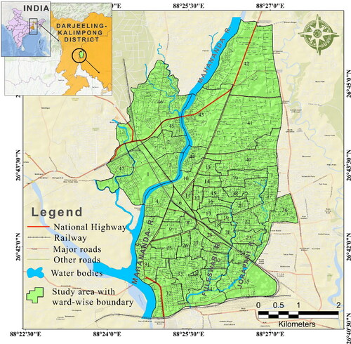
Siliguri, a city in West Bengal, India, is one of the most populous and fastest-growing metropolises. Its strategic position as the ‘gateway of north-eastern India’ is due to its location in a small corridor linking Bhutan in the north, Bangladesh in the south, and Nepal in the northwest section (District Census Handbook 2011; Bhattacharyya and Mitra 2013; Roy and Mandal 2020). Because of its advantageous location, the economy and people have expanded rapidly. It includes portions of West Bengal’s Darjeeling and Jalpaiguri districts. After Kolkata and Asansol, Siliguri is West Bengal’s third-biggest urban agglomeration. According to Indian Census, a city with a minimum population of 1,00,000 and above can be considered a Class-1 urban centre. Siliguri went from being a little town to a thriving commercial centre because of the entry of many new residents (Bose and Chowdhury 2020; Roy et al. 2021). Located in the foothills of the Himalayas, on the banks of the Mahananda River, its average elevation is 122 meters (400 feet). Siliguri Municipal Corporation covers around 41.9 km2 and is divided into 47 wards, expanding by a factor of five since 1931 as the city’s population has grown swiftly and densely (Roy et al. 2022). From over four lakhs in 2001 to over fife lakhs in 2011, the city’s population has increased faster than any other in India (Bhattacharyya and Mitra 2013). The city is generally a linear structure extended 9 kilometres long from north to south and more than 5 kilometres wide from east to west. Increasing temperatures, air pollution (Roy and Singha 2020; Roy et al. 2020) and noise pollution levels, population density, and other demographic characteristics all point to a degradation in the city’s environmental quality, which may be traced back to the area’s diverse environmental and socio-economic conditions (Biswas et al. 2020; Sarkar and Chouhan 2020; Halder and Bandyopadhyay 2021). This highlights the significance of urban planners and environmental managers having a comprehensive understanding of the city’s environmental quality over time (Hoque and Rohatgi 2022). Therefore, this rapidly expanding metropolis requires researchers and planners to keep a close eye on these environmental conditions, which can be accomplished through UEQ measurement and continuous environmental quality monitoring in parallel with the vibrant and prosperous economy of the city. The present study is a modest attempt to fulfil the gap in the UEQ assessment in the Siliguri city (Figure 1).

Figure 1. Location map of the study area with ward-wise boundary. The map also shows major roads, National highways, Railways and Major water bodies.

2.2. Development of dimensions and indicators for UEQ assessment

The Urban environment quality is a complex stature, developed with different interrelated, overlapping, and diversified components (Tao et al. 2019; Yibo et al. 2021). This complex, multi-factorial nature of the urban environment needs to be investigated through multi-dimensional strategies (Nichol and Wong 2009; Liang and Weng 2011; Fang et al. 2021). Therefore, the present study adopted the UEQ evaluation system using a modified approach based on those strategies. The development procedure holistically explores the issues and sustainability models for benefiting the urban environment and empowering the role of urban dwellers (Stossel et al. 2015; Fang et al. 2021; Yibo et al. 2021). From the different literature and experts’ opinion, we identified three significant dimensions, viz. eco-environmental quality (EEQ) (Kamp et al. 2003; Stossel et al. 2015; Javanbakht et al. 2021; Yibo et al. 2021; Pramanik et al. 2022), landscape and built-up quality (L&BU) (Liang and Weng 2011; Musse et al. 2018; Shen et al. 2022) and socio-economic quality (SEQ) (Kamp et al. 2003; Musse et al. 2018; Zandi et al. 2019) of the urban dwellers, used to measure the level of spatial heterogeneity of urban environment quality among the 47 spatial units of Siliguri city.

Initially, the three dimensions mentioned above cover by 23 indicators. However, the sorting process during the initial phase of analysis helps us to finalize the fifteen indicators. It methodologically enhanced the final output of UEQI. However, the selected dimensions majorly follow three pillars of the ideal indicators selection process suggested by different researchers (Wong 2014; Musse et al. 2018; Tao et al. 2019; Fang et al. 2021; Javanbakht et al. 2021), i.e. objective-oriented: capacity to measure the complex composite pattern of urban environment quality; availability: the indicators for these selected dimensions are readily available, extractable and understandable; reality-oriented: these selected indicators primarily reflect the reality of urban environment of the selected study site. The researchers checked and filtered it using the previous literature and preliminary tests.

The eco-environmental criteria are the most fundamental dimensions for the measurement of UEQ. It is because EEQ signifies and affects the core pattern of urban environment degradation by influencing the principle components of the environment as well as harming the quality of life and living pattern of urban dwellers (Musse et al. 2018; Sannigrahi et al. 2020; Javanbakht et al. 2021). The EEQ quality domain mainly comprises indicators that reflect the natural environmental quality, urban surface characteristics, and pollution level (LST, NDVI, NDWI, Air Quality Index, Green space, and distance from dumping ground). Musse et al. (2018) opined that these indicators were majorly extracted through Remote Sensing and GIS techniques. On the other hand, the landscape and built-up quality domain involve indicators relating to urban construction, structure, pressure on the land surface, and slum concentration (NDBI, household density, built-up percentage, noise pollution, and distance from slum). Urban landscapes significantly enhance the city’s environment and generate a pleasant impression of the city (Musse et al. 2018; Boori et al. 2021). Besides, Socio-economic factors are the key to maintaining an urban environment with the specification of neighbourhood environmental quality, residential quality of life, and effective health outcomes for the urban inhabitants (Fobil et al. 2010; Rao et al. 2012; Dongzagla 2022). Here, the socio-economic indicators were mainly selected from census enumeration to fabricate basic characteristics of the social and economic environment (educational status, population density, marginalized population, and unemployment).

2.3. Data source and its processing

A multisource non-spatial and spatial dataset of about 15 variables has been used to delineate UEQI, which can be divided into four categories, i.e. (1) Remote sensing data from Landsat 8 images, (2) GIS datasets, (3) census datasets and, (4) primary datasets including use of instruments and GPS surveys. The variables and indicators considered are provided in Table 1, based on the studied literature and the availability of data for the city. Among 15 variables, 67% are prepared using remote sensing and GIS database, and the remaining from other two sources. The Landsat data have been used for the preparation of Land surface temperature (LST), Normalized Difference Vegetation Index (NDVI), Normalized Difference Built-up Index (NDBI), Green index, and built-up percentage. The GIS database includes distance from slums and distance from dumping yards, while census data consist of population density, household density, educational status, marginalized population, and unemployed population. For Air Quality and Noise level dataset, we have selected 13 significant nodes of the study area and collected the data using an instrumental survey, which was later processed using a GIS environment. Initially, Landsat OLI image for the year 2021 with 30 m resolution was collected from USGS Earth explorer website and pre-processed using band composition, geometric, and radiometric corrections techniques (Salem et al. 2021). Subsequently, parameters like LST, NDVI, NDWI, NDBI, and Green index were calculated in the GIS environment. Figure 2 depicts the overall methodology for the present study.

Figure 2. Methodological flow chart adopted for the present study.

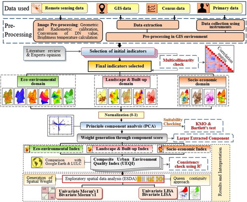
Table 1. Selected indicators for the present study with their relevance.

Domain	Indicators	Functional relation	Relevance and justification	Source
Eco-environmental quality	Land Surface Temperature (LST)	-ve	The quality of the urban environment and living space depends greatly on the urban thermal environment, as increasing LST significantly hampers the environmental quality and living satisfaction	Landsat 8 OLI
	Normalized Difference Vegetation Index (NDVI)	+ve	Increased NDVI suggest the improved urban environment with higher concentration of healthy green vegetation.
	Normalized Difference Water Index (NDWI)	+ve	NDWI is a widely used indicators that helps to understand the water feature and water stress to validate the condition of urban environment.
	Air Quality	-ve	Urban environmental quality relies on urban air quality, which indicates pollution levels in a city. Bad air quality degrades the urban ecosystem, human health, and living quality.	Primary instrumental survey
	Green Space Coverage	+ve	The availability of green space favours the urban environment by reducing surface temperature and mitigating pollutants. For city dwellers, it also suggests several social and psychological benefits.	Landsat 8 OLI
	Distance from Dumping Ground	-ve	Unplanned and open dumping harms the ecosystem by causing odour and destroying its aesthetics. Open landfill near human communities causes contamination, disease, and poor health.	Google Earth
Landscape and Built-up Environment	Normalized Difference Built-up Index (NDBI)	-ve	A higher NDBI indicates greater impervious layers, such as buildings and roads. Thus maximum NDBI values has a negative impact on the natural state and green ecology of the urban environment.	Landsat 8 OLI
	Household Density	-ve	Household density denotes the concentration of households depending on land availability. Maximum household density puts a greater strain on land, which negatively correlates with environmental quality.	Census
	Built-up Coverage	-ve	Built-up area and housing density are directly correlated; the greater the built-up coverage, the worse the environmental quality.	Landsat 8 OLI
	Noise Level	-ve	Urban noise harms the environment, ecology, and quality of life. Elevated noise level is a crucial problem for urban administration due to its adverse effects on human health, tranquillity, and beauty.	Primary instrumental survey
	Distance from Slums	-ve	Slum expansion threatens urban ecology and environmental quality by putting strain on electricity, water supply, and sewage capacity. Moreover, slum expansion causes overpopulation, garbage disposal issues, and hampering the aesthetic environment.	Google Earth
Socio-Economic	Population Density	-ve	High population density causes overcrowding and significantly strains urban space, resulting in congestion, air and noise pollution, and deforestation.	Census
	Literacy	+ve	Literacy and urban environmental quality are positively connected. High literacy rates indicate environmental awareness. They recommend ways to retain green space, minimize air pollution, reduce noise levels and improve overall well-being.
	Unemployment	-ve	Unemployment is a crucial socioeconomic factor associated with economic level and environmental quality. As urban unemployment rises, more people rely on natural resources. Besides, unemployment causes slums, disrupts urban ecology, and harms physical and mental health.
	Marginalized Population	-ve	Here, marginalized populations are Scheduled Caste and Scheduled Tribes population. The marginalised population has the least access to economic and institutional infrastructure in the city, which is linked to poverty, isolation, and environmental degradation.

For the preparation of LST, the first steps include the algorithm’s initial state is the entry of band 10. The tool utilizes the following calculations from the USGS website to get the top of atmosphere (TOA) spectral radiance (Lλ) after input of band 10 (Avdan and Jovanovska 2016), (1) $$L\lambda =M_L\mathrm{*}{Q}_{\text{cal}\mathrm{ }}+A_L-O_i,\mathrm{ }$$(1) where M_L represents the band-specific multiplicative rescaling factor, Q_cal is the Band 10 image, A_L is the band-specific additive rescaling factor, and Q_i is the correction for Band 10 (Barsi et al. 2014).

Secondly, TIRS band data be transformed from spectral radiance to brightness temperature (BT) using the thermal constants given in the metadata file once the digital numbers (DNs) have been transformed to reflection. The tool’s algorithm uses the following equation to transform reflectance into BT (Kumari et al. 2018). (2) $$BT=\frac{K_2}{\ln \hspace{0.17em}\left[\left(\frac{K_1}{L\lambda }\right)+1\right]}-273.15\mathrm{ }$$(2) where K₁ and K₂ are thermal conversion constants that are band-specifically defined in the metadata. The radiant temperature is adjusted by adding the absolute zero (about −273.15 °C) to get the values in Celsius.

In the next step, NDVI is calculated for emissivity correction. The NDVI employs the red and near-infrared bands and is the most common vegetation index used to categorize vegetation, non-vegetated regions, and aquatic bodies (Roy et al. 2021). The NDVI value is always between −1 and +1. Here, positive values near +1 suggest a high likelihood of dense plant cover and thick evergreens, while negative values near −1 imply bodies of water (Chatterjee and Majumdar 2022). NDVI derived using Eq. (3) $$\mathit{NDVI}=\mathrm{ }\frac{(\mathit{NIR}\mathrm{ }-\mathrm{ }\mathit{RED})}{(\mathit{NIR}\mathrm{ }+\mathrm{ }\mathit{RED})}\mathrm{ }$$(3)

After the NDVI is computed, the percentage of vegetation (PV) and emissivity (ε) must be computed, both of which are significantly correlated with the NDVI. According to Wang et al. (2015), P_v is computed as follows, (4) $$P_v=\left(\frac{\mathrm{NDVI}-{\mathrm{NDVI}}_{\mathrm{MIN}}}{{\mathrm{NDVI}}_{\mathrm{MAX}}-{\mathrm{NDVI}}_{\mathrm{MIN}}}\right)$$(4)

Since the land surface emissivity (LSE) is a scaling factor that scales blackbody radiance (Planck’s law) to predict emitted radiance, and it is the effectiveness of transmitting thermal energy across the surface into the atmosphere, it is necessary to know the LSE in order to estimate LST (Jiménez-Muñoz et al. 2006). As indicated, the calculation of the surface emissivity is done conditionally (Sobrino et al. 2004) (5) $${\epsilon }_{\lambda }={\epsilon }_{v\lambda }{P}_v+{\epsilon }_{s\lambda }\left(1-P_v\right)+C_{\lambda }\mathrm{ }$$(5)

Where C stands for surface roughness (C = 0 for homogeneous and flat surfaces) and is considered as a constant value of 0.005 (Sobrino and Raissouni 2000). Where ε_V and εs are the vegetation and soil emissivities, respectively.

The last step of retrieving the LST or the emissivity corrected land surface temperature Ts is computed as follows (Stathopoulou and Cartalis 2007) (6) $$T_s=\frac{\mathrm{BT}}{\left\{1+\left[\left(\frac{\lambda \mathrm{BT}}{\rho }\right)\ln \hspace{0.17em}{\epsilon }_{\lambda }\right]\right\}}\mathrm{ }$$(6) where Ts is the LST in Celsius (∘C) (Becker and Li 1990), BT is at-sensor BT (∘ C), λ is the wavelength of emitted radiance (for which the peak response and the average of the limiting wavelength (λ = 10.895) (Markham and Barker 1985) will be used), ελ is the emissivity calculated in (Barsi et al. 2014), and (7) $$p=\mathrm{h}\frac{c}{\sigma }=1.438\times {10}^{-2}mK\mathrm{ }$$(7) where σ is the Boltzmann constant (1.38 × 10⁻²³ J/K), h is Planck’s constant (6.626 × 10⁻³⁴ J s), and c is the velocity of light (2.998 × 10⁸ m/s) (Weng et al. 2004).

Subsequently, the NDWI values are significantly connected to plant moisture content and sensitivity to built-up lands, making it an excellent approximation for measuring plant water crisis (Roy et al. 2021). These numbers are important in assessing vegetation liquid water status calculations from space. The reflectance characteristics of green and dry plants are crucial to this state. The reflectance index ranges from −1 to +1 and is used to extract water bodies for satellite images using eq. (McFeeters 1996; Ashok et al. 2021). (8) $$\mathit{NDWI}=\frac{(\mathit{GREEN}-\mathit{NIR})}{(\mathit{GREEN}+\mathit{NIR})}\mathrm{ }$$(8)

The NDBI Index is a visual indicator used to assess urban regions, mainly built-up zones or artificial construction areas (Zheng et al. 2021). NDBI mapping primarily uses two bands: Short Wave Infrared and Infrared Band (Kulkarni and Vijaya 2021). This index is mainly used for built-up index mapping ranging from −1 to +1, with a positive value indicating the existence of artificial structures or built-up regions and a lower value indicating the existence of physical attributes. NDBI can be expressed as, (9) $$\mathit{NDBI}=\mathrm{ }\frac{(\mathit{SWIR}\mathrm{ }-\mathrm{ }\mathit{NIR})}{(\mathit{SWIR}\mathrm{ }+\mathrm{ }\mathit{NIR})}\mathrm{ }$$(9)

The Green Index (GI) is the proportion of greenness in each ward of the study area, based on the categorization of NDVI data (Gupta et al. 2012). Besides, Google earth image is also utilized for editing and vector modification. The final GI was calculated using the following equation (Singh 2018; Abutaleb et al. 2021). (10) $$GI=\sum _{i=1}^{n}G÷\sum _{i=1}^{n}A\mathrm{ }$$(10)

Where, G is the green space in square meter in i^th unit (ward) and A is the particular area of i^th unit(ward). Similarly, NDBI was used to calculate the built-up percentage in each ward of the study area.

Google Earth was utilized to delineate the dumping yard of the city, and a slum map was collected from the Municipal corporation office. Later, the ‘Euclidean Distance’ function from the GIS environment was performed. Similarly, for the preparation of population density, household density, educational status, marginalized population, and unemployed population data were collected from the Census of India, 2011. All these data are accessible in attribute format, which was included in the ‘Attribute table’ of the GIS platform to prepare final maps. An instrumental survey was conducted for the Air Quality and Noise measurement. These air quality and noise data were gathered in 2021 from 13 critical nodes across the city; later inverse distance weighting (IDW) interpolation method was employed in the GIS environment for further analysis. The IDW technique seems more accurate and consistent than any other technique for delineating air quality and noise level on a local scale (Harman et al. 2016; Jumaah et al. 2019). The present research utilizes a variety of datasets with different resolutions to get the intended results. However, the majority of the analysis done for this study was performed using satellite images (Landsat imageries) with a spatial resolution of 30 m. Therefore, to prevent any spatial output errors, all the selected indicators are transformed into the UTM Projection, WGS-84 Datum, Zone 45 N, with a uniform cell size of 30 m. Subsequently, the ‘Zonal statistics as Table’ tool was used to retrieve the data in the GIS environment. Finally, all the ward-wise retrieved data were transferred to Microsoft Excel for further evaluation.

2.4. Test of multicollinearity

Before running the multivariate model for spatial data, the indicators were tested for an issue of multicollinearity (Gebrekidan Abbay et al. 2018; Giacalone et al. 2018). Multicollinearity is a statistical test to check the level of correlation among the variables for the highest and most reliable statistical interpretations (Giacalone et al. 2018). Different techniques were used to test the multicollinearity problem, namely, correlation analysis employing Pearson’s correlation (Siddiquee et al. 2018), Spearman correlation, Kendal Correlation, Cramer’s V, and Variance Inflation Factors (VIF) (Gujarati and Porter 2003; Gebrekidan Abbay et al. 2018). For the present study, we used the Pearson correlation technique, suggested by Krishnan and Firoz (2020) and Malah and Bahi (2022) to check the multicollinearity of the 23 indicators initially selected for the Urban Environment Quality assessment. An effective Principle Component Analysis (PCA) results need a minimum correlation (r = 0.3) among the variables. However, for suitable statistical inference, we removed the indicators with low correlation (r < 0.3) and indicators with very high correlation (r > 0.9) (Pallant 2007; Krishnan and Firoz 2020). Based on the initial 23 indicators calculation, we removed eight variables due to multicollinearity issues from the subsequent analysis stage. Finally, out of 23 indicators, 15 were selected for the multivariate analysis employing Principle Component Analysis (PCA).

2.5. Indicator normalization

Indicator normalization is necessary for analyzing spatial data due to the heterogeneous nature of measurement units. The normalization technique transformed the entire datasets with an identical value range between 0 and 1 (OECD 2008; Majumder 2021). For the study, we used a normalization technique called ‘homogenization’ and ‘non-dimensionalization’ that helps to eliminate the dimensionality of the selected indicators (Malghan 2020).

It is necessary to reveal that all the selected indicators were not uniformly related to urban environment quality (UEQ). For example, NDVI, NDWI, green space, and literacy indicate a healthier influence on urban environment quality, positively associated with UEQ. However, distance from slums, LST, air quality, noise level, and population density indicate a negative association with urban environment quality (Table 1). So, it is necessary to normalize each indicator using either Equations (11) or (12) (Majumder 2021). Equation (11) was employed when an indicator had a positive association with UEQ, whereas Equation (12) was employed when an indicator had a negative association with UEQ (Majumder 2021). (11) $$X_{\mathit{SDi}}=\frac{\left(X_i-\mathrm{ }{X}_{\min }\right)}{\left(X_{\max }-\mathrm{ }{X}_{\min }\right)}\mathrm{ }$$(11) (12) $$X_{\mathit{SDi}}=\frac{\left(X_{\max }-\mathrm{ }{X}_i\right)}{\left(X_{\max }-\mathrm{ }{X}_{\min }\right)}\mathrm{ }$$(12)

Where, $X_{\mathit{SDi}}$ = Normalize value for ‘i’ of ‘X’ indicator; $X_i$ = Raw value for ‘i’ ward of ‘X’ indicator; $X_{\max }$ = Maximum valu of ‘X’ indicator; $X_{\min }$ = Minimum value of ‘X’ indicator.

2.6. Principle component analysis for spatial data

Principle component analysis is a multilevel statistical analysis that transforms the datasets based on the linear association and explains the variability of latent information of the input datasets (Pearson 1901; Liang and Weng 2011; Greco et al. 2019). Several researchers used PCA to derivate the urban environment scenario and associated sustainability (Nichol and Wong 2009; Liang and Weng 2011; Krishnan and Firoz 2020; Yibo et al. 2021; Pramanik et al. 2022). Here, the Spatial Principle Component Analysis was performed to generate weights of the normalized variable for the preparation of the composite layer of UEQ for Siliguri City.

A prerequisite for PCA is generating the Kaiser Meyer Olkin (KMO) test and Bartlett’s Test of Sphericity (Table S1). Kaiser Meyer Olkin (KMO) test and Bartlett’s Test of Sphericity is an essential test to check the variance of sample adequacy (Tobias & Carlson 1969; Kaiser 1974) and generate an identity matrix to test the probability of partial correlation between the variables (Bartlett 1950). Another essential measure of PCA is eigenvalues for the retention of components for further analysis. Kaiser (1960) suggested to derive several components with eigenvalues greater or equal to one. The PCA output (Varimax rotation with Kaiser Normalization) encompasses a minimum number of components (eigenvalue >/= 1) where the first component explains the highest possible variance of the input variables, the second component explains the second-highest possible variance, and so on (Greco et al. 2019). Finally, the rotated component score with the highest loading of the original individual variable is the best choice to employ as indicator weight to interpret the decomposition characteristics of correlated indicators for environmental quality assessment for the different municipal units (Table 2).

Table 2. Rotated component loading score of each indicators.

	Component
	1	2	3	4
Distance from dumping ground (mts)	−.122	−.214	.759	−.031
LST (degree C)	−.515	.573	.281	.000
NDBI	−.709	.154	.064	.250
NDWI	−.101	−.682	.261	.182
NDVI	.896	−.018	−.132	−.037
Population density	.566	−.014	.625	.309
Household density	.555	−.108	.596	.385
Literate (%)	−.270	.794	.070	.054
Wardwise % of Green space	.841	−.228	.119	.002
Air quality Average	−.017	−.065	−.052	−.856
NOISE (db)	.099	.050	.120	−.821
Built-up area (%)	.838	−.328	.256	.004
Unemployed population	−.457	.596	−.337	.221
Marginalized Population	−.348	.598	−.316	.477
Distance from Slums (mts)	−.075	−.142	−.631	.250

2.7 Construction of urban environment quality index (UEQI)

Construction of the UEQI was carried out by combining the three dimensions, i.e. EEQ, L&BU, and SEQ. These three dimensions comprise 15 indicators that positively or negatively influence the quality of the urban environment quality. The derived principal components score was used as indicator weight to develop three-dimensional indices that further being used to construct a synthetic UEQI. The obtained weights (larger extracted components) through PCA for spatial data and the dimensional index were calculated as follows, (13) $${DI}_{\mathit{EQAi}}=\frac{\left(a_{x1}{w}_{x1}+\mathrm{ }{a}_{x2}{w}_{x2}+\mathrm{ }{a}_{x3}{w}_{x3}+\dots +\mathrm{ }{a}_{xn}{w}_{xn}\right)}{N}\mathrm{ }$$(13)

Here, DI_EQAi is the dimensional index for environmental quality assessment for ‘i’ ward. Here, the dimensional index comprises three distinct components, i.e. EEQ, L&BU, SEQ. Further, ‘a_x1, a_x2, a_x3,…., a_xn’ is the normalized value of ‘x’ indicator for each individual spatial units (ward). ‘w_x1, w_x2, w_x3,…., w_xn’ is the weight of ‘x’ indicator. Here, the weight is derived from highest factors loading of each variable of respective components. ‘N’ is the number of variable used to compute the dimensional index for each component. So, the index of three derived dimensions for each ward is the average of the sum of the product of indicator values and the respective weights.

In the next step, the environment quality was calculated using the average sum estimation technique using the values of dimensional indices mentioned above. The Urban Environment Quality Index (UEQI) is the composite representation of EEQ, L&BU, and SEQ. The UEQI was constructed using the following equation, (14) $$\mathit{UEQI}=\frac{\left({EE}_Q+{L\&BU}_Q+\mathrm{ }{SE}_Q\right)}{N_{\mathit{inc}}}\mathrm{ }$$(14)

UEQI is nothing but the average dimensional index. Here, EEQ, L&BU, and SEQ are the individual dimensional indices, and N_inc is the number of indices.

2.8. Exploratory spatial data analysis (ESDA): spatial autocorrelation and spatial clustering

Exploratory spatial data analysis (ESDA) focuses on the unique aspects of geographic data and seems to be an elaboration of data exploration (Dall’erba 2009; Sarwar 2021). Considering the values of the employed variable in the immediate neighbourhood, ESDA correlates a particular variable to a specific location (Anselin et al. 2007). ESDA corresponds to identifying the underlying clustering pattern of spatial data and summarizing the main findings of the data based on the neighbourhood location. The popular method used for this purpose is called Spatial Autocorrelation, which signifies the presence or absence of spatial relationships among the employed indicators (Anselin et al. 2007); however, it is being measured by using Moran’s I statistics with the application of LISA. Here, the two types of spatial autocorrelation techniques (Univariate Moran’s I, LISA, and Bivariate Moran’s I, LISA) was used to explore the spatial relationship of dimensional index values. Univariate Moran’s I with LISA was used to check clustering patterns among individual domains in a univariate way, i.e. EEQ, L&BU, SEQ, and UEQI (analysing the distribution of just one variable at a time throughout the area); whereas, Bivariate Moran’s I with LISA used to check spatial cluster among two variables in a bivariate way, i.e. EEQ with UEQI, L&BU with UEQI, SE with UEQI (analysing the distribution of two variables throughout the area) (Moura and Fonseca 2020). The outcome result helps us to explore the spatial heterogeneity and relation between the domains mentioned above and their relation with UEQ. For that purpose, generating a spatial weight matrix is essential to measure the strength of the relationship among the spatial unit (Anselin et al. 2007; Anselin 2010).

2.8.1. Spatial connectivity and spatial weights matrix

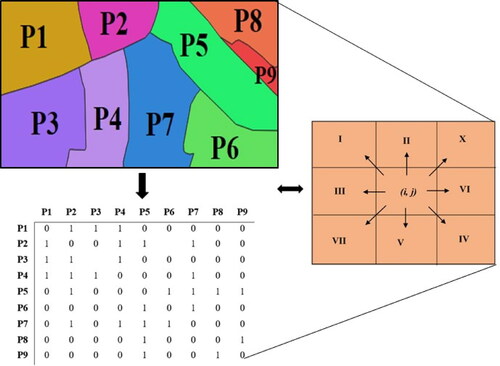
The different researchers used various techniques to develop the spatial weights matrix to reflect the pattern of neighbourhood relation (Anselin et al. 2007). The study considered one weight technique called queen contiguity spatial weight metrics, because of the least fit of the other weight technique like rock contiguity and inverse distance. The spatial weight (Wij) is non-zero when ‘i’ and ‘j’ are neighbours; for other cases, it was zero (Anselin 2010; Sarwar 2021; Kumar et al. 2022). The concept of Queen Contiguity weights is to identify the associate boundary between the spatial units, which means if a unity of ‘i’ share a common boundary (north, east, west, south, and corners and verticals) with another unit of ‘j,’ they might be considered as neighbour and giver a weigh of 1 (Figure 3) (Sarwar 2021; Kumar et al. 2022). The Queen Contiguity weights are defined by the following representation (Kumar et al. 2022), $$W_{ij\mathrm{ }=\mathrm{ }}\{\begin{array}{c}1, \mathit{bnd} \left(i\right)\cap \mathit{bnd} \left(j\right) \ne \varnothing \\ 0, \mathit{bnd} \left(i\right)\cap \mathit{bnd} \left(j\right) \ne \varnothing \end{array}$$

Figure 3. Spatial Weight using Queen Contiguity approach.

Moran’s I statistics is the way to measure spatial autocorrelation. The Univariate Moran’s I generally identify the spatial autocorrelation of the used spatial units based on the individual variable selection concerning the spatial location (Anselin et al. 2007). The study used to identify the pattern of spatial association of individual dimensions, i.e. EEQ, L&BU, SE, and UEQI. Here, Moran’s I statistics examine the local association by considering the spatial clusters of the input variables. The formula of Univariate Moran’s I statistics are as follows (Kumar et al. 2022), (15) $$\text{Univariate}\mathrm{ }\text{Moran}\text{’s I }=\frac{n}{S_O}\times \frac{{\mathrm{\Sigma }}_i{\mathrm{\Sigma }}_j{W}_{ij}\left(x_i-\overline{X}\right)\left[x_j-\overline{X}\right]}{{\mathrm{\Sigma }}_i{\left[x_i-\overline{X}\right]}^2}$$(15)

Where, x = variable of interest and X = mean of x; n = number of spatial units; W_ij = standardized weight matrix between observation i and j with zeroes on the diagonal; and S_o = aggregate of all spatial weights, i.e. S_o = ${\sum }_i{\sum }_j$ W_ij

Bivariate Moran’s I identify the spatial clustering and correlation between two variables based on the corresponding spatial location. Here, the technique was employed to examine the pattern of cluster and associated heterogeneity among the dimension of environmental quality with UEQI. The formula of bivariate Moran’s I are as follows, (16) $$\text{Bivariate}\mathrm{ }\text{Moran}\text{’s I}=\frac{n}{S_O}\times \frac{{\mathrm{\Sigma }}_i{\mathrm{\Sigma }}_j{W}_{ij}\left(x_i-\overline{X}\right)\left[Y_j-\overline{Y}\right]}{{\mathrm{\Sigma }}_i{\left[y_i-\overline{Y}\right]}^2}$$(16)

Where, x and y = variables of interest; X = mean of x; Y = mean of y; n = number of spatial units; W_ij = standardized weight matrix between observation i and j with zeroes on the diagonal; and S_O = aggregate of all spatial weights, i.e. S_o = ${\sum }_i{\sum }_j$ W_ij $$I=\{\begin{array}{c}+1 \text{ Maximum Degree of Clustering }\\ 0 \text{ Randomness }\\ -1 \text{ Highest Degree of Randomness and Dispersion }\end{array}$$

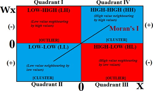
The values of Moran’s I fall between −1.0 (indicating perfect dispersion) to +1.0 (perfect correlation) (Figure 4). The Index would be zero if positive cross-product values offset negative cross-product values, indicating a random spatial pattern (Kumar et al. 2022). The Moran’s Index will be positive if the spatial clustering of the values in the dataset tends to be positive (high values cluster adjacent to other high values; low values cluster adjacent to other low values). The Index will be negative if high values tend to be near the low ones and repel other high ones (Anselin 1988; Anselin et al. 2007; Sarwar 2021).

Figure 4. Quadrant of Moran’s I Scatter plot.

2.8.2. Univariate and bivariate local indicators of spatial auto-correlation (LISA)

LISA statistics help measure the degree of spatial clustering and the occurrence of outliers in a defined area (Moura and Fonseca 2020). In structured datasets, LISA is used to define specific patterns of spatial association based on the local location and decompose the pattern with global autocorrelation measures, including Moran’s statistics (Anselin 2010). LISAs are widely utilized in various domains to detect geographical outliers or clusters. The study employed two techniques of LISA, univariate and bivariate, in terms of the nature and objective of the study.

Univariate Local Indicators of Spatial Auto-correlation statistics measure the spatial association of the neighbouring feature based on a single parameter with a specific spatial location of the study. Here, the eco-environment, built-up and landscape, socio-economy, and UEQI were used as input features to identify the map of spatial clusters and potential outliers and decompose the findings with Moran statistics. The measure of univariate LISA [Ii] is constructed by the following equation (Kumar et al. 2022), (17) $$\text{Univariate}\mathrm{ }\text{LISA:}\mathrm{ }{I}_i=\frac{n\cdot \left[x_i-\overline{X}\right]}{{\mathrm{\Sigma }}_i{\left[x_i-\overline{X}\right]}^2}{\mathrm{\Sigma }}_j{w}_{ij}\left[x_j-\overline{X}\right]$$(17)

Bivariate Local Indicators of Spatial Auto-correlation is another useful tool to identify the nature of the spatial association between the exposure and outcome variables with their locational reference (Singh et al. 2011; Kumar et al. 2022). The present study used UEQI as an outcome variable to identify the corresponding spatial pattern with the influence of three exposure variables, i.e. EEQ, L&BU, and SEQ. The equation of bivariate LISA [Ii] is represented below (Kumar et al. 2022), (18) $$\text{Bivariate}\mathrm{ }\text{LISA:}\mathrm{ }{I}_i=\frac{n\cdot \left[x_i-\overline{X}\right]}{{\mathrm{\Sigma }}_i{\left[y_i-\overline{Y}\right]}^2}{\mathrm{\Sigma }}_j{w}_{ij}\left[y_i-\overline{Y}\right]$$(18)

A high positive z-score for a space indicates that the neighbouring features have similar values (either high values or low values). A low negative z-score for a space indicates a statistically significant spatial data outlier. Based on this principle, the LISA provides four major types of spatial clustering and outliers with the statistically significant result: High-High (HH) Cluster of high values, Low-Low (LL) cluster of low values, High-Low (HL) outliers of high values with neighbouring low values, and Low-High (LH) outliers of low values with neighbouring high values (Singh et al. 2011; Sarwar 2021).

3. Results

3.1. Initial data exploration and statistical analysis

In the present research, fifteen environmental and socioeconomic factors were chosen from the census, RS-GIS & Primary survey to create an UEQ index, as mentioned in the methodology section. However, to determine the degree of redundancy, the values of each indicator were arranged in a matrix and checked using Pearson correlation analysis. It is required to use multivariate approaches like principal component analysis.

The correlation matrix result of the variables indicates a high positive correlation among green space, NDVI, population density, household density, literacy, unemployment, and marginalized population; a moderate positive correlation exists among air quality, NDWI, NDBI, and built-up (Figure 5). Although, air quality, NDVI, NDBI, noise, and built-up negatively correlated. Before conducting PCA, two preliminary checks were executed to identify the suitability of the data for further analysis. These two tests includes Bartlett’s test of sphericity and the Kaiser-Mayer-Olkin (KMO) measure of sampling adequacy to check the validity of the results. KMO result varies from 0 to 1.0 (Nardo et al. 2005). Large KMO (>0.5) is recommendable for the principal component analysis (PCA) because it dramatically explains the correlation between pairs of variables and indicates the presence of a robust partial correlation (Kaiser 1960; Nardo et al. 2005). Empirically, large chi-square values with a statistically significant result at p < 0.05 for Bartlett’s test are considered suitable for PCA analysis (Tabachnick et al. 2007). As per our analysis, the value of the KMO was 0.722, more significant than the recommended value of 0.5 (Kaiser 1960; Nardo et al. 2005). Additionally, Bartlett’s test of sphericity was also significant at p = 0.00 with a considerable Chi-square value of 492.061, which established that the multivariate factor analysis is appropriate for the study.

Figure 5. Correlation matrix of the variables. The red colour showing positive correlation and blue showing negative correlation.

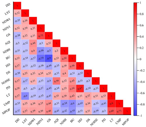
The extraction (h2) of the indicators indicates higher loading with a recommendable value of above 0.4 (Dharmaratne and Attygalle 2018). The highest extraction was observed for the percentage of built-up, followed by household density, NDVI, population density, and marginalized population (Table S2). The table shows four components with an eigenvalue greater than 1 (followed Kaiser criteria for selecting components, Kaiser 1960), explaining about 70 percent of the cumulative variance in the data (Table S3). The first component explains the largest variance (25.558 percent), which included four indicators (NDBI, NDVI, percentage of green space, and percentage of built-up) with the largest rotated loadings. The second component (16.038 percentage of variance) includes LST, NDWI, literacy, unemployment, and marginalized population. The third and the last component covered four indicators (distance from dumping ground, household density, distance from slum, and population density) and two indicators (average air quality and noise level), respectively.

Table 3. Summary of Regression analysis for model consistency.

Model	Predictors	Coefficients	R^2	Constant	Significance
Urban Environmental Quality Index (UEQI)	NDVI	.762	0.832	9.820	.000
	Literacy	.365			.004
	Distance from Dumping Ground	.556			.000
	Air Quality	−.546			.000

3.2. Variation in domains and its associated factors

According to the Figure 6a, only 34% (16 wards) of Siliguri city have a good EEQ, mainly distributed over the north-western and south-western parts. The significant factors related to good EEQ include low temperature, high NDVI values (correspondence to maximum vegetation), low air pollution, and higher coverage of green space (Roy and Singha 2020; Jiang et al. 2021; Malah and Bahi 2022). Thus, the wards in the NW and SW part of the city comprises factors such as low to moderate LST, high vegetation covers, high NDVI values, low air quality index, and maximum concentration of green space (Figure S1a–f). Besides, moderate to worst environmental quality mainly covers the city’s central part, owing to adverse environmental factors.

Figure 6. Urban environmental quality domains (a) Eco-environmental quality index, (b) Landscape and Built-up index, (c) Socio-economic index.

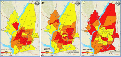
On the other hand, Figure 6b reveals that 30% (14 wards) of the city, primarily located in the northern and western part, has a better L&BU. Contrastingly, the majority of the wards (36%) located in the central part of the city have poor landscapes & built-up environments. These central areas of the city experience a maximum concentration of slums (along the Mahananda, Jorapani, and Fuleshwari rivers, and along the railway stations of Junction and Siliguri town stations), maximum household density, elevated noise level, high NDBI values, and maximum built-up areas (Figure S2a–e). The housing density is proportionate to built-up areas and NDBI values; the higher the concentration of built-up areas lowers the environmental quality (Faisal and Shaker 2017a; Boori et al. 2021). Further, the complexity of geographical distribution influences the growth of slum settlements, leading to a decline in environmental quality (Joseph et al. 2014; Surya et al. 2020a). Similarly, noise levels and surrounding built-up are strongly correlated with each other (Yuan et al. 2019), and noise levels are predicted to be higher in locations with the most densely and highly developed built-ups (Sakieh et al. 2017; Tong and Kang 2021). Besides, the northern and southern areas experience a better landscape and built-up environment due to low household density, minimum slum concentration, minimum noise level, and a lower percentage of built-up.

Interestingly Figure 6c reveals that the north-central and south-central part of the study area reveals good socio-economic status mainly due to the high literacy rate and low marginalized and unemployed population (Figure S3). However, better socio-economic condition does not ameliorate the quality of the environment in those parts of the city, as colossal population pressure is the single dominant factor that results in the deterioration of the environment. The population density of these north and south central parts varies from 20,000 to 48,000 person per sq. km approximately, with 28% of the total population of the study area. Previous research by Weber and Sciubba (2019), Boori et al. (2021), and Hussain et al. (2022) have also shown that population density can be a single dominating factor that degrades environmental quality. However, the central part (wards 18, 20 & 28), the N-W part, and the S-E part of the city have poor socio-economic conditions. These areas have low to moderate population density, low levels of literacy, and maximum concentration of marginalized and unemployed populations.

3.3. Urban environmental quality index (UEQI) and model consistency

In order to create a single synthetic index, all three of the domains mentioned above must be taken into account since they reflect the UEQ of Siliguri city in various ways. The UEQI map created for the present study region demonstrates that the area’s overall environmental quality is s substandard in general (Figure 7). It reveals that 34% (16 wards) of the total area is under poor environmental quality, followed by 42.5% (20 wards) under moderate, and only 23.5% (11 wards) have good urban ambiance. The good UEQ is primarily located in the northern (Salugara area, Patiram Jote, Dashratpally, Punjabi para, Prakash Nagar, some parts of Pradhannagar area) and southern part of the city (Babupara area, Railway colony, and Kashmir colony). Figure 7b,d–f, reveals that these good zones are defined by a high vegetation density, less impermeable surfaces, maximum open spaces, parks, and minimum slum concentration. Since these northern and southern parts are located at the outskirt of the city, which is away from the congestion; as a result, they have the least air and noise levels, minimum LST values, low concentration of built-up areas, and, more importantly, less population and household densities.

Figure 7. Composite map of Urban Environmental Quality (UEQ) of Siliguri City. The UEQ map compares with present Land Use Land cover (LULC) and Google earth images.

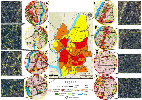
In contrast to the northern and southern portions, the moderate UEQ class is distributed over the N-W part (Champasari area, Mallaguri, Siliguri town station, parts of Mahananda para), the north and south central part (Millanpally, Deshbandhupara, parts of Subhas pally, Rabindrasarani, Ghogomali, Dabgram) of the city. These areas are associated with moderate vegetation cover, moderate to high pollution levels, moderate LST, and NDBI values. Besides several business and retail services, entertainment hubs, maximum public service distribution, moderate unemployment, and moderate to high population and household density adversely affected the urban environment.

The UEQ tends to decline towards the downtown area, which is considered the most congested and haphazard part of the city (Baghajotin colony, Jantanagar, Mahananda para, Ganganagar, Saktigarh, Khalpara, Subhas pally, Hakimpara, Arabinda pally, parts of Dabgram, Haidarpara, Shibrampally, Durganagar). According to Figure 7a, c, g and h, the localities in these regions are distinguished by maximum density of urban built-up (includes residential, commercial, and mixed), maximum concentration of slums, low green space, maximum pollution levels, congested roads, and elevated temperature. The maximum built-up intensity causes havoc, congestion, and traffic in the central part of the city, which is also associated with high pollution levels (Roy and Singha 2020). Moreover, high land surface temperature values are another element that contributes to the poor environmental quality in certain local bodies (Sharma et al. 2021; Su et al. 2021). Some of the neighbourhoods in the present research area located in central parts have poor environmental quality and high LST values between 33 and 36 °C. The primary causes of high temperature in those areas are mainly due to the construction of buildings and roads, extreme traffic congestion, and reduction of green covers. Previous studies by Portela et al. (2020), Shah et al. (2021), and Yin et al. (2022) and have also proved that the construction of impervious surfaces and encroachment of green covers result in the reduction of permeability of surface, consequences in extreme surface temperature. Besides, the interaction between environmental and neighbourhood socio-economic status is another crucial factor in determining the UEQ (Liang and Weng 2011; Musse et al. 2018; Jamal and Ajmal 2020).

Interestingly, the N & S central section of the city is unable to sustain the environmental quality despite having higher socio-economic variables (i.e. high literacy, low unemployment, and low marginalised population). The UEQ continues to deteriorate in these areas due to enormous population pressure as it prevents sustaining and recovering the central areas’ environmental quality. Around 36% of the total population (1,84,982) resides within these 16 wards of Siliguri city. Consequently, such high population intensity puts significant pressure on the environment, which eventually lowers the city’s UEQ. Besides, Table S4 indicates the ward wise scores for all three domains including the UEQI.

Table 4. Summary of ANOVA for factors causing spatial heterogeneity.

Domains	Indicators	F Statistics	Significance
Eco-environmental quality	NDVI	3.86	0.016
	NDWI	3.20	0.033
	LST	3.31	0.026
	Green Space	5.72	0.002
	Distance from dumping grounds	4.35	0.009
	Air quality	3.368	0.041
Landscape and Built-up Quality	NDBI	0.657	0.583
	Household Density	4.05	0.013
	Ward wise Built-up	8.95	0.001
	Noise level	8.64	0.001
	Distance from slum	1.34	0.273
Socio-economy	Population Density	4.62	0.007
	Literacy	4.052	0.023
	Unemployment	3.87	0.015
	Marginalized Population	0.583	0.629

The constructed UEQ model’s consistency is evaluated using the r-squared value of regression analysis (Musse et al. 2018; Krishnan and Firoz 2020), where the predictor variables are independent factors with the highest loading under each component, and the outcome variable is the UEQI value. According to Hair et al. (2011), the R² value of the latent variable with values of 0.25, 0.50, and 0.75 may be regarded as weak, moderate, and significant, respectively. The regression analysis results (Table 3) show that the model is acceptable since it accounts for almost 83% of the variance of the developed UEQ index, with an R² value of 0.832. Besides, the model is also statistically significant since the p-values for all the predictors are less than 0.05.

3.4 Spatial clustering pattern of UEQI domains using exploratory spatial data analysis (ESDA)

3.4.1. Univariate Moran’s I and LISA analysis

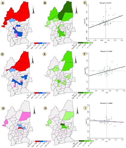
A visual representation of univariate spatial association can be seen here in Figure 8a–l. This figures illustrates univariate LISA (cluster and significance map) and univariate local Moran of the selected outcome domains, i.e. eco-environment (Figure 8a–c), landscape and built-up (Figure 8d–f), socio-economy (Figure 8g–i), and Urban Environment Quality Index (Figure 8j–l) across the 47 spatial administrative units in Siliguri city. In previous discussions, we have stated that the LISA yields two types of clusters (HH and LL) and two types of outliers (HL and LH). A noticeable fact is that the High-High (HH) clusters are popularly called 'hotspots,' and the Low-Low (LL) is popularly called 'coldspots.'

Figure 8. Univariate LISA map, its significance level (green map) and Moran scatter plot. (a-c) Eco-environmental domain, (d-f) Landscape and built-up domain, (g-i) Socio-economic domain and, (j-l) Composite Urban environmental quality.

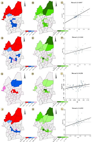
The univariate ESDA indicates that the eco-environmental domain was calibrated with the largest Moran’s value, 0.567 (p < 0.001), among the four selected outcome components. In contrast, the socio-economic domain corresponds to the lowest Moran’s value of 0.250. It suggests that the eco-environmental domain was significant spatial autocorrelation, with positive spatial association and clustering among the spatial units (wards) of Siliguri city. Figure 8a and b indicates northern part of Siliguri city emerged as a hotspot or high-high clusters, and the central part of the city emerged as coldspots with low-low clusters in the eco-environmental domain. The results suggest that the geographical clustering with high values of eco-environmental domain signifies the best quality of the environment in six adjoining wards. However, the central part of the city corresponds with the lowest performance in eco-environment quality, rationalizes the degradation process of the urban environment (includes high temperature, low greenery, low NDVI, and bad air quality), and provides the worst eco-environment quality for the urban inhabitants. Further, the visualization indicates that one ward was low with high neighbourhood values in the eco-environmental domain, which means it identifies as Low-High outliers and suggests a bad quality environment adjoining with satisfactory eco-environment.

According to the Figure 8d–f, shows the univariate spatial association of landscape and built-up domain. The univariate Morain’s I result of 0.269 indicates a clustering tendency with moderate randomization among the geographical units in terms of the employed variable of landscape and built-up quality index. The results of the univariate LISA visualization indicate that the northern part of the city corresponds with a geographically significant hotspot (high values adjoining high value neighbouring wards). The result replicates the findings of the previous outcomes and suggests good quality environmental conditions experienced by the urban dwellers residing in the northern part of Siliguri city. Additionally, two wards emerged as outliers (LH) of low values corresponding with high values. The central part of the city identifies six wards as coldspots, which means a Low-Low cluster. It signifies that the central part of the city has significantly low performance in landscape and built-up domain, and the region is more concentrated with built-up that drastically alternates the city’s environmental quality. A striking feature is that in the central part, a ward of high values in landscape and built-up domain corresponds with low-value results as High-Low (HL) outliers.

A univariate LISA cluster map of the socio-economic status of urban inhabitants (Moran’s I = 0.250) indicates geographical clustering at a moderate level (Figure 8g–i). The LISA map displays two types of clusters, two wards with low-low clusters and five wards with high-high clusters. The low-low clusters were observed in the upper part of the city, where the environmental quality is comparatively better than in the other part of the city. On the other hand, high-high clusters were identified in the central part of Siliguri city. Generally, a higher socio-economic status is observed around the city’s central part, mainly due to higher literacy rates, low concentration of marginalized populations, and more economic opportunities.

Figure 8j–l shows Moran’s scatter plots for the final composite Urban Environment Quality Index (UEQI); Moran’s index value of UEQI was 0.393 (p < 0.001). A univariate LISA cluster map of UEQI identified six High-High clusters and five Low-Low clusters among the 47 wards in Siliguri city. Most of the HH clusters were significant at 0.01 level, while most of the LL clusters were significant at 0.05 level. The results indicate that geographic clustering of the highest values of UEQI in the northern part of Siliguri city. It suggests that the wards in the northern part of the city are experiencing satisfactory environmental quality compared to the other part of the city. Further, the central part of the city experiences the worst environmental quality due to the clustering of low values. Additionally, ward number 2 and 19 were identified as Low-High outliers (low UEQI values surrounded by high UEQI) and High-Low outliers (high UEQI values surrounded by low UEQI), respectively. The overall spatial patterns of clusters in all the maps are similar in nature except for socio-economic quality. The univariate LISA analysis suggests that the northern part of the city was best in terms of the urban environment quality. However, the socio-economic domain suggests more concentration in the wards with comparatively poor environmental quality. In all the cases, many spatial units (wards) with no significant results. Additionally, the southern part of Siliguri city was found geographically insignificant, and the random nature of spatial heterogeneity in terms of the four outcome variables.

3.4.2. Bivariate Moran’s I and LISA analysis

The LISA, Moran Local Index and bivariate results (clusters and significance maps) were presented in Figure 9a–i indicating the spatial association and dependencies of UEQI with predicted variables (eco-environment, landscape and built-up, and socio-economy) for the 47 spatial units (wards) in Siliguri city. The result revealed the comparative characteristics between the exposure and the outcome variable, which provide valid ground to identify the spatial heterogeneity of urban environment quality based on the locational weights.

Figure 9. Bivariate LISA map, its significance level (green map) and Moran scatter plot. (a-c) UEQ and Eco-environmental domain, (d-f) UEQ and Landscape and built-up domain, (g-i) UEQ and Socio-economic domain.

Figure 9a–c, of LISA map shows the positive spatial autocorrelation (Moran’s I: 0.372) of eco-environment and UEQI. The LISA map indicates 13 spatial clusters (six hotspots and seven coldspots) with three outliers (one low-high and two high-low). The northern part of Siliguri city emerged as a hotspot, which signifies high eco-environmental quality wards surrounded by high UEQI. The results suggest that the better eco-environmental quality causes the higher value of UEQI in the region compared to the other parts of the city. Although the central part of the city emerged as a coldspot, there were areas with low eco-environmental quality surrounded by areas of low UEQI.

The results presented in Figure 9d–f show spatial clustering and spatial outliers of landscape and built-up with UEQI across the 47 spatial units of Siliguri city. The figure displays Moran’s index value of 0.264 at p < 0.001 significance level. The bivariate LISA map shows that out of 47 wards, four wards were high-high (hotspot) cluster, five wards was low-low clusters (coldspot), and most of the wards emerged as insignificant results. The results suggest that the high-high clusters were high landscape and built-up index values surrounded by high UEQI, while the coldspots areas was low landscape and built-up index values surrounded by low UEQI. The results substantiate the findings that good landscape and built-up quality (with a low concentration of slums, low household density, minimum noise levels, and low built-up percentage) enhance the overall quality of the urban environment. Here, the high values clusters are identified in the northern part of the city, whereas the low-quality environmental cluster is found in the central part. Further, few wards identified as outliers majorly correspond with the areas of high-high and low-low clusters.

The results in Figure 9g–i show spatial clustering and spatial outliers of the socio-economic domain with UEQI (Moran’s index: −0.069). The results of Moran suggest a negative spatial association, with a higher tendency to randomization among the outcome and predictor variables. The negative spatial correlation signifies the geographic pattern of employed values in a manner of dissimilar values, as high locational values have low values, which corresponds with high and low neighbouring values. The figure portrays the LISA map, indicating that only one ward emerged as a significant hotspot at a 0.01 significant level, and some wards were high-low and low-high outliers. The results suggest that socio-economic factors were matters of random choice, and it hardly has a spatial impact on the quality of the urban environment in Siliguri city. However, the population pressure in the central part influences the spatial pattern of the urban environment.

3.5. Factors causing spatial heterogeneity

In order to identify the factors causing spatial heterogeneity in the urban environmental quality among the wards of Siliguri city, we decomposed indicator values to UEQI level were used Analysis of Variance (ANOVA) (Table 4). The results of the ANOVA test suggest that 12 factors out of 15 factors significantly influence the spatial difference in urban environment quality. The spatial heterogeneity was significantly caused by NDVI, NDWI, LST, green space coverage, dumping ground, and air quality corresponding to the decomposition level of eco-environmental quality. Furthermore, spatial differences in household density, built-up percentage, noise, population density, literacy, and unemployment significantly correspond to landscape, built-up, and socio-economic quality. The analysis confirms that the spatial variation among the factors related to eco-environment, landscape and built-up, and socio-economy functionally influence the heterogeneous spatial pattern of urban environment quality among the 47 spatial units of Siliguri city.

4. Discussion

The findings of the present study are consistent with other studies that focused on creating indices for modelling UEQ (Faisal and Shaker 2017b; Musse et al. 2018; Krishnan and Firoz 2020; Ghosh and Sarkar 2022; Pramanik et al. 2022), environmental vulnerability (Nandy et al. 2015; Zou and Yoshino 2017) and urban sustainability (Malah and Bahi 2022).

The UEQ of Siliguri city is generally poor due to its haphazard expansion and unplanned structure. Besides, the city’s urban design is an organic pattern characterized by narrow streets, low-rise buildings, and unstructured infrastructural services. The localities around the railway station terminals (Siliguri Town station and Junction station) are densely populated, congested, and overburdened with infrastructural services, which results in the urban development along transportation corridors, particularly towards the highway, major roads, and so on (CDP Report Siliguri 2015). Furthermore, the growth pressure in the core area negatively influenced the green cover and open spaces of the city. The central business district is defined by a high population and household density in the neighbourhoods around the train station. Therefore, rapid urban development, huge population concentration, and the commercialization of space might be the primary culprits for degrading the UEQ (Sofeska 2016; Pramanik et al. 2022). Previous work by Hussain et al. (2022) and Coluzzi et al. (2022) demonstrates that population density may be a primary driving element in urban environmental deterioration. Besides, the city is distinguished by medium-rise and high-density residents in the centre city and low-rise, moderate-density housing on the outskirts. However, the previous decade has witnessed the expansion of central business districts’ construction of multistory residential and commercial buildings along Sevoke road, Bidhan road, and Hillcart road, creating massive pressure on the neighbourhood environment. The concentration of maximum household densities are associated with overcrowding, negatively impacting urban residents and threatening the environment (Ferreira et al. 2018; Sarkar and Bardhan 2020). In contrast, the findings reveals that the peripheries of the city experience good UEQ, primarily due to the availability of vegetation, low population pressure, low household density, and minimum LST. Due to dense urbanization and lack of greenery, the city’s downtown is warmer, followed by a medium-density zone with moderate vegetation and low-density zones with significantly lower temperatures on the periphery (CDP Report Siliguri 2015; Roy et al. 2021). Other important factors that deteriorate the UEQ of Siliguri city are air pollution and elevated noise levels.

Huge traffic volume and massive congestion are the primary causes of air pollution in Siliguri city. Besides, the city’s road system is disorganized, with a greater concentration of intercity and local routes. Furthermore, the road system lacks a clear order since most metropolitan routes also serve as interstate traffic. Therefore, a haphazard road network causes significant vehicle traffic, particularly in the central part of Siliguri. The major corridors with elevated levels of air pollution are Sevoke road, Hill cart route, Bardhaman road, Bidhan road, SF road, and so on. Besides, diesel-powered city autos are another prominent cause of rising pollution levels (Roy and Singha 2020). In addition to these factors, Siliguri’s pollution level is also affected by extensive road construction and the development of multistory buildings, which ultimately worsens the environment. Besides, the Noise levels that negatively influence the environment are much greater along automobile traffic arteries such as Hill Cart Road, Bidhan Road, Champasari road, Sevoke Road, and Bardhaman Road than in residential areas. In the SMC region, a considerable amount of high-frequency noise is provided by a huge number of automobiles blowing the horns, with the sound intensity ranging between 80 and 90 dBA. The sound intensity along national highways ranges from 90 to 100 dBA, although it is under the permissible limits of 50 to 60 dBA in residential areas. However, during festive seasons the noise level is significantly high due to loudspeakers.

Another factor contributing to the deterioration of UEQ is the concentration of Slums. Dilapidated structures and abandoned buildings in urban areas are characterized as slums. These haphazard constructions harm the environment in various ways (Omoboye and Festus 2020). Residents of slums face significant environmental challenges, such as blocked sewers, stagnant ponds, insufficient water supply, and inadequate garbage disposal and sanitation (Surya et al. 2020a; Khan 2022). Slums in Siliguri city can be found around the river banks, on railway property, and in the city centre near the railway station. The existence of disorganized structures in the urban slums endangers environmental safety. Due to the affordable rent, low-income individuals in the city gravitate into the inner city slums. As a result, the slum regions of Siliguri are marked by unhygienic and structural chaos. The low-income residents who live in subpar, decaying, and squatter communities are linked to encroachment, garbage disposal issues, traffic congestion, water shortages, environmental degradation, and building deterioration in Siliguri city. Besides, the issue of unscientific solid waste disposal in the landfill without being treated causes environmental annoyance in the nearby residential neighbourhoods.

The socio-economic factors also influence the environmental quality of the urban areas (Faisal and Shaker 2017a); for instance, a high socio-economic level, low marginalized population, excellent urban planning, and low population density consequences in good environmental quality (Musse et al. 2018). Besides, factors like better job opportunities and higher literacy rates also tend toward better urban ambiance (Krishnan and Firoz 2020; Surya et al. 2020b). Although having better socio-economic characteristics (i.e. low unemployment, high literacy, and low marginalised population), in the N & S central area of the present study, the city is still incapable of maintaining the environmental quality. Because the considerable impact of intense population thwarts the core regions’ environmental quality from being sustained and recovered; as a result, the UEQ in these areas gradually tends to decline. In contrast, the city’s periphery regions have significant marginalization, high unemployment, and poor literacy, yet the UEQ in these areas seems to be favourable primarily due to low population pressure.

5. Conclusion and recommendations

Only a few urban areas can deliver the best outcomes to their residents while simultaneously minimizing their detrimental impacts on the natural environment. The majority, on the other hand, are finding it more challenging to keep up with population expansion and urbanization while attempting to govern, develop, and create infrastructure to serve their neighbourhoods. Because these rapidly growing urban centres are associated with environmental degradation; thus, the present study is critical for evaluating UEQ. The present study used the GIS environment in conjunction with statistical techniques to investigate the complexity and spatiality of UEQ, which can be ideal for environmental management, and policy-making toward sustainable city government. The adopted synthetic index derived using the proposed approach is reproducible and can be applied to different cities worldwide.

Siliguri is a rapidly progressing city, experienced the accelerated progression of urbanization, which has positively impacted the developmental perspective of the urban inhabitants. However, the unsustainable growth is accompanied by massive pressure on the urban environment and more costs to the future development and welling of the city inhabitants. Based on the inspiration, the present study is to prepare a multilevel synthetic index for evaluating UEQ and the underlying spatial heterogeneity in terms of UEQ. The study utilizes a set of 15 indicators appropriate for measuring the urban environment. All these indicators are classified under three inter-connected domains: eco-environmental, landscape and built-up, and socio-economy. In the latter stage, the spatial autocorrelation among the three domains and UEQI were accessed using Exploratory Spatial Data Analysis (ESDA) technique. The ESDA approach for the study involved localized univariate and bi-variate spatial association checks through Moran index and LISA. Furthermore, the determinant factors affecting spatial heterogeneity were identified using ANOVA.

The study’s findings suggest that the northern part of north-western and some southern parts of Siliguri city experience good environmental quality. The wards such as 10, 32, 34, 41, 42, 43, 45, and 47 are environmentally friendly and ideal for sustainable city growth and environment management. The findings identify spatially significant 'hotspots’ and 'coldspots’ across the 47 wards of Siliguri city based on the eco-environment quality, landscape, built-up quality, socio-economic quality, and UEQI. Moreover, the hotspots emerged in the upper part of the city except in the socio-economic domain, which signifies better environmental quality in these wards far from the central business part of the city. As a result, problems like urban environmental degradation can be explained through local statistics that account for localized issues and challenges.

However, UEQ management and measurement are complex issues corresponding to different dynamic concepts and tools. Noteworthy that our study provides a fundamental and sophisticated base for both conceptual and methodological context and minimizes the complexity of the quantification of UEQ. Furthermore, future studies on community-level participation and engagement are recommended to obtain a holistic overview of the urban environment and ascertain the opinions of the public about the realities of what issues are more critical at the ground level. Understanding the various environmental quality parameters in the city enables intervention in areas with more significant environmental problems to be prioritized. It also allows for better zoning and planning as one of the numerous strategies urban planners adopt to govern cities’ physical and environmental aspects. In order to mitigate the negative consequences of urbanization, it also encourages the creation of new investigations and initiatives in other fields, such as environmental studies, engineering, and architecture. Even at the local level, UEQI measurement enables the monitoring procedure to be robust at both spatial and temporal scales, providing a reliable mechanism for urban policymakers and planners to attain sustainable urban management goals. Although, the findings of this research with the idea of spatial clustering will undoubtedly encourage municipal authorities to conduct robust monitoring and more extensive planning in ecologically susceptible areas of cities. In addition, this study will serve as a foundation for future studies and policymaking about one of the SDGs’ most crucial tenets, i.e. the creation of sustainable cities and communities. With this approach, cities can better prepare for the future, resulting in more resilient infrastructure.

Credit authorship

S.R. A.B. and S.M. – Writing Original Draft, Conceptualization, Formal analysis, Investigation, Methodology, Software, Visualization, Review & Editing; I.R.C – Review & Editing, H.G.A. – Funding allocation, Review & Editing H.A., A.D., and M.M. – Review & Editing. All authors have read and agreed to the published version of the manuscript.

Acknowledgments

The author wishes to thank the Department of Geography and Applied Geography, University of North Bengal (India) for providing necessary facilities to carry out this study. The authors would also like to thanks University of Tartous (Syria), Damascus University (Syria), University of Tishreen (Syria) and Qassim University (Saudi Arabia) for their collaboration. Besides the authors would like to acknowledge all the Governmental reports and data without which it is impossible to find such novel results. Finally, the authors would like to express their heartfelt appreciation to the editor and two anonymous reviewers for their informative remarks and ideas, which greatly assisted in improving the manuscript.

Data availability statement

The data used in this study is available on request with the corresponding author and is not available publicly due to ongoing research.

Disclosure statement

No potential conflict of interest was reported by the authors.

References

- Abutaleb K, Mudede MF, Nkongolo N, Newete SW. 2021. Estimating urban greenness index using remote sensing data: a case study of an affluent vs poor suburbs in the city of Johannesburg. Egypt J Remote Sens Space Sci. 24(3):343–351.
- Anselin L, Sridharan S, Gholston S. 2007. Using Exploratory spatial data analysis to leverage social indicator databases: the discovery of interesting patterns. Soc Indic Res. 82(2):287–309.
- Anselin L. 1988. Spatial econometrics: methods and models. (Vol. 4). Springer Science & Business Media. doi:10.1007/978-94-015-7799-1.
- Anselin L. 2010. Local indicators of spatial association—LISA. Geograp. Anal. 27(2):93–115.
- Ashok A, Rani HP, Jayakumar KV. 2021. Monitoring of dynamic wetland changes using NDVI and NDWI based landsat imagery. Remote Sens Appl: Soc Environ. 23:100547.
- Avdan U, Jovanovska G. 2016. Algorithm for automated mapping of land surface temperature using LANDSAT 8 satellite data. J Sens. 2016:1–8.
- Barsi JA, Schott JR, Hook SJ, Raqueno NG, Markham BL, Radocinski RG. 2014. Landsat-8 thermal infrared sensor (TIRS) vicarious radiometric calibration. Remote Sens. 6(11):11607–11626.
- Barthel S, Isendahl C, Vis BN, Drescher A, Evans DL, van Timmeren A. 2019. Global urbanization and food production in direct competition for land: leverage places to mitigate impacts on SDG2 and on the Earth System. Anthropoc Rev. 6(1-2):71–97.
- Bartlett MS. 1950. Tests of significance in factor analysis. Brit J Stat Psychol. 3(2):77–85.
- Becker F, Li ZL. 1990. Towards a local split window method over land surfaces. Remote Sens. 11(3):369–393.
- Bhattacharyya DB, Mitra S. 2013. Making Siliguri a walkable city. Procediasoc Behav Sci. 96:2737–2744.
- Biswas K, Chatterjee A, Chakraborty J. 2020. Comparison of air pollutants between Kolkata and Siliguri, India, and its relationship to temperature change. J Geovis Spat Anal. 4(2):1–15.
- Boori MS, Choudhary K, Paringer R, Kupriyanov A. 2021. Eco-environmental quality assessment based on pressure-state-response framework by remote sensing and GIS. Remote Sens Appl: Soc Environ. 23:100530.
- Bose A, Chowdhury IR. 2020. Monitoring and modeling of spatio-temporal urban expansion and land-use/land-cover change using markov chain model: a case study in Siliguri Metropolitan area, West Bengal, India. Model Earth Syst Environ. 6(4):2235–2249.
- Camagni R, Capello R, Nijkamp P. 1998. Towards sustainable city policy: an economy-environment technology nexus. Ecol Econ. 24(1):103–118.
- CDP Report Siliguri. 2015. City Development Plan for Siliguri 2041. Capacity Building for Urban Development Project, Ministry of Urban Development. http://siligurismc.in/userfiles/file/siliguri-CDP-final-report-29April15.pdf.
- Chatterjee U, Majumdar S. 2022. Impact of land use change and rapid urbanization on urban heat island in Kolkata city: a remote sensing based perspective. J Urban Manage. 11(1):59–71.
- Choudhary BK, Tripathi AK, Rai J. 2019. Can ‘poor’cities breathe: responses to climate change in low-income countries. Urban Clim. 27:403–411.
- City BL, Assessment E. 2010. Urbanization and health. Bull World Health Organ. 88(4):245–246.
- Cohen B. 2006. Urbanization in developing countries: current trends, future projections, and key challenges for sustainability. Technol Soc. 28(1-2):63–80.
- Coluzzi R, Bianchini L, Egidi G, Cudlin P, Imbrenda V, Salvati L, Lanfredi M. 2022. Density matters? Settlement expansion and land degradation in Peri-urban and rural districts of Italy. Environ Impact Assess Rev. 92:106703.
- Dall’erba S. 2009. Exploratory spatial data analysis. Int Encycloped Hum Geograph. 683–690.
- Dharmaratne MA, Attygalle MDT. 2018. Improving the statistical capacity index: a statistical approach. Am J Appl Math Stat. 6(3):80–95.
- District Census Handbook. 2011. Village and town directory. West Bengal: Directorate of Census Operations.
- Dongzagla A. 2022. Socioeconomic and demographic factors affecting urban household access to improved water and sanitation in Ghana. GeoJournal. 87(6):4763–4773.
- Elmqvist T, Fragkias M, Goodness J, Güneralp B, Marcotullio PJ, McDonald RI, Wilkinson C. 2013. Urbanization, biodiversity and ecosystem services: challenges and opportunities: a global assessment.
- Faisal K, Shaker A. 2017a. An investigation of GIS overlay and PCA techniques for urban environmental quality assessment: a case study in Toronto, Ontario, Canada. Sustainability. 9(3):380.
- Faisal K, Shaker A. 2017b. Improving the accuracy of urban environmental quality assessment using geographically-weighted regression techniques. Sensors. 17(3):528.
- Fang X, Shi X, Gao W. 2021. Measuring urban sustainability from the quality of the built environment and pressure on the natural environment in China: a case study of the Shandong Peninsula region. J Cleaner Prod. 289:125145.
- Ferreira CS, Walsh RP, Ferreira AJ. 2018. Degradation in urban areas. Curr Opin Environ Sci Health. 5:19–25.
- Fobil J, May J, Kraemer A. 2010. Assessing the relationship between socioeconomic conditions and urban environmental quality in Accra, Ghana. Int J Environ Res Public Health. 7(1):125–145.
- Gebrekidan Abbay A, Rutten R, Azadi H, Witlox F. 2018. How social status contributes to sustainable livelihoods? An empirical analysis in Ethiopia. Sustainability. 11(1):68.
- Ghosh A, Sarkar S. 2022. Assessing land use change and potential environmental quality in Chandernagore Municipal Corporation, India. Environ Dev Sustain. 24(8):10255–10288.
- Ghosh S, Das A, Hembram TK, Saha S, Pradhan B, Alamri AM. 2020. Impact of COVID-19 induced lockdown on environmental quality in four indian megacities using landsat 8 OLI and TIRS-derived data and mamdani fuzzy logic modelling approach. Sustainability. 12(13):5464.
- Giacalone M, Panarello D, Mattera R. 2018. Multicollinearity in regression: an efficiency comparison between Lp-norm and least squares estimators. Qual Quant. 52(4):1831–1859.
- Greco S, Ishizaka A, Tasiou M, Torrisi G. 2019. On the methodological framework of composite indices: a review of the issues of weighting, aggregation, and robustness. Soc Indic Res. 141(1):61–94.
- Gujarati DN, Porter DC. 2003. Basic econometrics, 4th ed. McGraw-Hill: New York, NY.
- Güneralp B, Reba M, Hales BU, Wentz EA, Seto KC. 2020. Trends in urban land expansion, density, and land transitions from 1970 to 2010: a global synthesis. Environ Res Lett. 15(4):044015.
- Gupta K, Kumar P, Pathan SK, Sharma KP. 2012. Urban Neighborhood Green Index–A measure of green spaces in urban areas. Landscape Urban Plann. 105(3):325–335.
- Hair JF, Ringle CM, Sarstedt M. 2011. Indeed a silver bullet. J Market Theor Pract. 19(2):139–152. PLSSEM MTP1069-6679190202.
- Halder B, Bandyopadhyay J, Banik P. 2021. Monitoring the effect of urban development on urban heat island based on remote sensing and geo-spatial approach in Kolkata and adjacent areas, India. Sustain Citi Soc. 74:103186.
- Halder B, Bandyopadhyay J. 2021. Air quality fluctuation monitoring and statistical data analysis during COVID-19 pandemic in Siliguri city, India. J Air Pollution Health. 6(3):197–208.
- Harman BI, Koseoglu H, Yigit CO. 2016. Performance evaluation of IDW, Kriging and multiquadric interpolation methods in producing noise mapping: a case study at the city of Isparta, Turkey. Appl Acoust. 112:147–157.
- Hasnine M. 2020. An analysis of urban sprawl and prediction of future urban town in urban area of developing nation: case study in India. J Indian Soc Remote Sens. 48(6):909–920.,
- Hoque I, Rohatgi S. 2022. Identification of potential urban residential area by integrating AHP and WCL in RS and GIS environment: a case study of Siliguri Municipal Corporation and Its Buffer of 7 km, West Bengal. J Indian Soc Remote Sens. 50(8):1437–1456.
- Hussain M, Usman M, Khan JA, Tarar ZH, Sarwar MA. 2022. Reinvestigation of environmental Kuznets curve with ecological footprints: empirical analysis of economic growth and population density. J Public Affair. 22(1):e2276.
- Jain M, Korzhenevych A. 2020. Urbanisation as the rise of census towns in India: an outcome of traditional master planning? Cities. 99:102627.
- Jamal S, Ajmal U. 2020. Assessing the relationship between neighbourhood socio-economic status and environmental quality. In Urban health risk and resilience in Asian cities. p. 445–459. Springer, Singapore.
- Javanbakht M, Darvishi Boloorani A, Kiavarz M, Neisany Samany N, Zebardast L, Zangiabadi M. 2021. Spatial-temporal analysis of urban environmental quality of Tehran, Iran. Ecol Indic. 120:106901.
- Jiang L, Liu Y, Wu S, Yang C. 2021. Analyzing ecological environment change and associated driving factors in China based on NDVI time series data. Ecol Indic. 129:107933.
- Jiménez-Muñoz JC, José A, Sobrino A, Gillespie D, Sabol, WT, Gustafson. 2006. Improved land surface emissivities over agricultural areas using ASTER NDVI. Remote Sens Environ. 103(4):474–487.
- Joseph M, Wang F, Wang L. 2014. GIS-based assessment of urban environmental quality in Port-au-Prince, Haiti. Habitat International. 41:33–40.
- Jumaah HJ, Ameen MH, Kalantar B, Rizeei HM, Jumaah SJ. 2019. Air quality index prediction using IDW geostatistical technique and OLS-based GIS technique in Kuala Lumpur, Malaysia. Geomatics Nat Hazards Risk. 10(1):2185–2199.
- Kaiser HF. 1960. The application of electronic computers to factor analysis. Educat Psycho Meas. 20(1):141–151.
- Kaiser HF. 1974. An index of factorial simplicity. Psychometrika. 39(1):31–36.
- Kamp IV, Leidelmeijer K, Marsman G, Hollander AD. 2003. Urban environmental quality and human well-being Towards a conceptual framework and demarcation of concepts; a literature study. Landscape Urban Plann. 65(1-2):5–18.
- Kattel GR, Elkadi H, Meikle H. 2013. Developing a complementary framework for urban ecology. Urban Forest Urban Green. 12(4):498–508.
- Khan MA. 2022. Livelihood, WASH related hardships and needs assessment of climate migrants: evidence from urban slums in Bangladesh. Heliyon. 8(5):e09355.
- Krishnan VS, Firoz CM. 2020. Regional urban environmental quality assessment and spatial analysis. J Urban Manage. 9(2):191–204.
- Kulkarni K, Vijaya PA. 2021. NDBI based prediction of land use land cover change. J Indian Soc Remote Sens. 49(10):2523–2537.
- Kumar P, Kundu S, Bawankule R. 2022. District level geospatial analysis of utilization of ICDS services among children in India. Front Public Health. 10:874104.
- Kumar R, Verma A, Shome A, Sinha R, Sinha S, Jha PK, Kumar R, Kumar P, Das S, Sharma P, et al. 2021. Impacts of plastic pollution on ecosystem services, sustainable development goals, and need to focus on circular economy and policy interventions. Sustainability. 13(17):9963.
- Kumari B, Tayyab M, Mallick J, Khan MF, Rahman A, Shahfahad, Salman. 2018. Satellite-driven land surface temperature (LST) using Landsat 5, 7 (TM/ETM + SLC) and Landsat 8 (OLI/TIRS) data and its association with built-up and green cover over urban Delhi, India. Remote Sens Earth Syst Sci. 1(3-4):63–78.,
- Leeson GW. 2018. The growth, ageing and urbanisation of our world. Population Age. 11(2):107–115.
- Liang B, Weng Q. 2011. Assessing urban environmental quality change of Indianapolis, United States, by the remote sensing and GIS integration. IEEE J Sel Top Appl Earth Observations Remote Sens. 4(1):43–55.
- Liang L, Wang Z, Li J. 2019. The effect of urbanization on environmental pollution in rapidly developing urban agglomerations. J Cleaner Prod. 237:117649.
- Lu L, Weng Q, Guo H, Feng S, Li Q. 2019. Assessment of urban environmental change using multi-source remote sensing time series (2000–2016): a comparative analysis in selected megacities in Eurasia. Sci Total Environ. 684:567–577.
- Majumder AK, Hossain ME, Islam MN, Sarwar MI. 1970. Urban environmental quality mapping: a perception study on Chittagong Metropolitan City. Kathmandu Univ J Sci Eng Technol. 3(2):35–48.
- Majumder S. 2021. Spatial pattern of multi-dimensional regional disparities in the level of socio-economic development in West Bengal: a geographical analysis. Geos Ind. 6(3):260–230.
- Malah A, Bahi H. 2022. Integrated multivariate data analysis for Urban Sustainability Assessment, a case study of Casablanca city. Sustain Citi Soc. 86:104100.
- Malghan D. 2020. On the normalization of dimensioned variables in ecological economics. Ecol Econ Soc. 1(1):17–31.
- Markham BL, Barker JL. 1985. Spectral characterization of the landsat thematic mapper sensors. Int J Remote Sens. 6(5):697–716.
- McFeeters SK. 1996. The use of the Normalized Difference Water Index (NDWI) in the delineation of open water features. Int J Remote Sens. 17(7):1425–1432.
- Meyer N, Auriacombe C. 2019. Good urban governance and city resilience: an afrocentric approach to sustainable development. Sustainability. 11(19):5514.
- Mnisi PT. 2020. The context and approaches of biodiversity conservation: a debate of its impacts on poverty alleviation in communities close to Skukuza Game Reserve, South Africa International Conference on Public Administration and Development Alternatives (IPADA).
- Moura ACM, Fonseca BM. 2020. ESDA (Exploratory Spatial Data Analysis) of vegetation cover in urban areas—Recognition of vulnerabilities for the management of resources in urban green infrastructure. Sustainability. 12(5):1933.
- Musse MA, Barona DA, Rodriguez LMS. 2018. Urban environmental quality assessment using remote sensing and census data. Int J Appl Earth Obs Geoinf. 71:95–108.
- Nandy S, Singh CDKK, Das KK, Kingma NC, Kushwaha SPS. 2015. Environmental vulnerability assessment of eco-development zone of Great himalayan National Park, himachal Pradesh, India. Ecol Indic. 57:182–195.
- Nardo M, Saisana M, Saltelli A, Tarantola S. 2005. Tools for composite indicators building. Eur Comission ISPRA. 15(1):19–20.
- Newman P, Jennings I. 2012. Cities as sustainable ecosystems: principles and practices. London: Island Press.
- Nichol J, Wong MS. 2009. Mapping urban environmental quality using satellite data and multiple parameters. Environ Plann B. 36(1):170–185.
- OECD. 2008. Handbook on constructing composite indicators methodology and user guide. Organisation for Economic Co-Operation and Development, ISBN 978-92-64-04345-9.
- Omoboye IF, Festus IA. 2020. Urban slums: environmental sustainability at A Cross Road.
- Pacione M. 2003. Urban environmental quality and human wellbeing—a social geographical perspective. Landscape Urban Plann. 65(1-2):19–30.
- Pallant J. 2007. SPSS survival manual, a step by step guide to data analysis using SPSS for windows. 3rd ed. Sydney: McGraw Hill.
- Paul S, Majumdar N. 2022. Assessment of road network connectivity and accessibility using gis and remote-sensing in Siliguri City, West Bengal, India. J Asiatic Soc Mumbai. 96:119–135.
- Pearson K. 1901. On lines and planes of closest fit to systems of points in space. Philosophical Magazine Series. 2(11):559–572.
- Portela CI, Massi KG, Rodrigues T, Alcântara E. 2020. Impact of urban and industrial features on land surface temperature: evidences from satellite thermal indices. Sustain Citi Soc. 56:102100.
- Portney KE. 2015. Sustainability. London (UK): MIT Press. ISBN-9780262331418.
- Pramanik S, Areendran G, Punia M, Sahoo S. 2022. Spatio-temporal pattern of urban eco-environmental quality of Indian megacities using geo-spatial techniques. Geocart Int. 37(17):5067–5090.
- Profiroiu CM, Bodislav DA, Burlacu S, Rădulescu CV. 2020. Challenges of sustainable urban development in the context of population Growth. EJSD. 9(3):51–51.
- Rahman A, Kumar Y, Fazal S, Bhaskaran S. 2011. Urbanization and quality of urban environment using remote sensing and GIS techniques in East Delhi-India. JGIS. 03(01):62–84.
- Rao KRM, Kant Y, Gahlaut N, Roy PS. 2012. Assessment of quality of life in Uttarakhand, India using geospatial techniques. Geocart Int. 27(4):315–328.
- Ritchie H, Roser M. 2018. Urbanization. Our world in data.
- Roy S, Bose A, Chowdhury IR. 2022. Darkness under the city lights: a qualitative study on the life of urban homelessness, evidence from Siliguri city of West Bengal, India. GeoJournal. 1–23.
- Roy S, Bose A, Singha N, Basak D, Chowdhury IR. 2021. Urban waterlogging risk as an undervalued environmental challenge: an Integrated MCDA-GIS based modeling approach. Environ Challen. 4:100194.
- Roy S, Mandal G. 2020. The problems of elderly residing in slums: a case study on Siliguri municipality. Indian J Gerontol. 34(3):313–332.
- Roy S, Singha N, Majumdar N, Roy B. 2020. Lockdown due to COVID-19 pandemic improves overall air quality: an evidence based study from Siliguri Metropolitan, West Bengal, India. Curr World Environ. (3):15. DOI
- Roy S, Singha N. 2020. Analysis of ambient air quality based on exceedance factor and air quality index for Siliguri City, West Bengal. Curr World Environ. 15(2):236–246.
- Sahoo G, Wani AM, Swamy SL, Roul PK, Dash AC, Sharma A. 2022. Livelihood strategy and sustainability aspects in industrialization as a source of employment in rural areas. In Social morphology, human welfare, and sustainability. Springer, Cham; p. 643–670.
- Sakieh Y, Jaafari S, Ahmadi M, Danekar A. 2017. Green and calm: modeling the relationships between noise pollution propagation and spatial patterns of urban structures and green covers. Urban Forest Urban Green. 24:195–211.
- Salem M, Bose A, Bashir B, Basak D, Roy S, Chowdhury IR, Alsalman A, Tsurusaki N. 2021. Urban expansion simulation based on various driving factors using a logistic regression model: delhi as a case study. Sustainability. 13(19):10805.
- Sannigrahi S, Zhang Q, Joshi PK, Sutton PC, Keesstra S, Roy PS, Pilla F, Basu B, Wang Y, Jha S, et al. 2020. Examining effects of climate change and land use dynamic on biophysical and economic values of ecosystem services of a natural reserve region. J Clean Prod. 257:120424.
- Sarkar A, Bardhan R. 2020. Socio-physical liveability through socio-spatiality in low-income resettlement archetypes-A case of slum rehabilitation housing in Mumbai, India. Cities. 105:102840.
- Sarkar A, Chouhan P. 2020. Modeling spatial determinants of urban expansion of Siliguri a metropolitan city of India using logistic regression. Model Earth Syst Environ. 6(4):2317–2331.
- Sarwar A. 2021. Mapping out regional disparities of reproductive health care services (RHCS) across Pakistan: an exploratory spatial approach. Asia-Pac J Reg Sci. 5(3):825–849.
- Shach-Pinsly D, Bindreiter S, Porat I, Sussman S, Forster J, Rinnerthaler M. 2021. Multiparametric analysis of urban environmental quality for estimating neighborhood renewal alternatives. UP. 6(4):172–188.
- Shah A, Garg A, Mishra V. 2021. Quantifying the local cooling effects of urban green spaces: evidence from Bengaluru, India. Landscape Urban Plann. 209:104043.
- Shao Q, Weng SS, Liou JJ, Lo HW, Jiang H. 2019. Developing a sustainable urban-environmental quality evaluation system in China based on a hybrid model. IJERPH. 16(8):1434.
- Sharma R, Pradhan L, Kumari M, Bhattacharya P. 2021. Assessing urban heat islands and thermal comfort in Noida City using geospatial technology. Urban Clim. 35:100751.
- Shen C, Hou H, Zheng Y, Murayama Y, Wang R, Hu T. 2022. Prediction of the future urban heat island intensity and distribution based on landscape composition and configuration: a case study in Hangzhou. Sustain Citi Soc. 83:103992.
- Siddiquee MN, Sivaramakrishnan K, Wu Y, de Klerk A, Nazemifard N. 2018. A statistical approach dealing with multicollinearity among predictors in microfluidic reactor operation to control liquid-phase oxidation selectivity. React Chem Eng. 3(6):972–990.
- Singh A, Pathak P, Chauhan RK, Pan W. 2011. Infant and child mortality in india in the last two decades: a geospatial analysis. PLoS One. 6(11):e26856.
- Singh KK. 2018. Urban green space availability in Bathinda City, India. Environ Monit Assess. 190(11):1–17.
- Sobrino JA, Jiménez-Muñoz JC, Paolini L. 2004. Land surface temperature retrieval from LANDSAT TM 5. Remote Sens Environ. 90(4):434–440.
- Sobrino JA, Raissouni N. 2000. Toward remote sensing methods for land cover dynamic monitoring: Application to Morocco. Int J Remote Sens. 21(2):353–366.
- Sofeska E. 2016. Relevant factors in sustainable urban development of urban planning methodology and implementation of concepts for sustainable planning (Planning documentation for the Master Plan Skopje 2001–2020). Procedia Environ Sci. 34:140–151.
- Stathopoulou M, Cartalis C. 2007. Daytime urban heat islands from Landsat ETM + and Corine land cover data: an application to major cities in Greece. Solar Energy. 81(3):358–368.
- Stossel Z, Kissinger M, Meir A. 2015. Assessing the state of environmental quality in cities – A multi-component urban performance (EMCUP) index. Environ Pollut. 206:679–687.
- Su H, Han G, Li L, Qin H. 2021. The impact of macro-scale urban form on land surface temperature: An empirical study based on climate zone, urban size and industrial structure in China. Sustain Citi Soc. 7:103217.
- Sudhira HS, Nagendra H. 2013. Local assessment of Bangalore: graying and greening in Bangalore–impacts of urbanization on ecosystems, ecosystem services and biodiversity. In Urbanization, biodiversity and ecosystem services: challenges and opportunities, p. 75–91. Springer, Dordrecht.
- Surya B, Hadijah H, Suriani S, Baharuddin B, Fitriyah AT, Menne F, Rasyidi ES. 2020b. Spatial transformation of a New City in 2006–2020: perspectives on the spatial dynamics, environmental quality degradation, and socio—economic sustainability of local communities in Makassar City, Indonesia. Land. 9(9):324.
- Surya B, Saleh H, Suriani S, Sakti HH, Hadijah H, Idris M. 2020a. Environmental pollution control and sustainability management of slum settlements in Makassar City, South Sulawesi, Indonesia. Land. 9(9):279.
- Tabachnick BG, Fidell LS, Ullman JB. 2007. Using multivariate statistics. Vol. 5, p. 481–498. Boston (MA): Pearson.
- Tao Y, Li F, Crittenden J, Lu Z, Ou W, Song Y. 2019. Measuring urban environmental sustainability performance in China: a multi-scale comparison among different cities, urban clusters, and geographic regions. Cities. 94:200–210.
- Tobias S, Carlson JE. 1969. Brief report: bartlett’s test of sphericity and chance findings in factor analysis. Multivariate Behav Res. 4(3):375–377.
- Tong H, Kang J. 2021. Relationship between urban development patterns and noise complaints in England. Environ Plan B Urban Anal City Sci. 48(6):1632–1649.
- Ullah S, Ahmad K, Sajjad RU, Abbasi AM, Nazeer A, Tahir AA. 2019. Analysis and simulation of land cover changes and their impacts on land surface temperature in a lower Himalayan region. J Environ Manage. 245:348–357.
- Wang F, Qin Z, Song C, Tu L, Karnieli A, Zhao S. 2015. An improved mono-window algorithm for land surface temperature retrieval from Landsat 8 thermal infrared sensor data. Remote Sens. 7(4):4268–4289.
- Weber H, Sciubba JD. 2019. The effect of population growth on the environment: evidence from European regions. Eur J Popul. 35(2):379–402.
- Weng Q, Lu D, Schubring J. 2004. Estimation of land surface temperature–vegetation abundance relationship for urban heat island studies. Remote Sens Environ. 89(4):467–483.
- Weng Q, Quattrochi DA. 2018. Urban remote sensing. Wiley-IEEE Press.
- Weng Q. 2019. Techniques and methods in urban remote sensing. CRC press, ISBN 9780367572044.
- WHO. 2010. Why urban health matters (No. WHO/WKC/WHD/2010.1). World Health Organization.
- Wong C. 2014. Indicator selection criteria. In Michalos AC. eds. Encyclopedia of quality of life and well-being research. Springer, Dordrecht.
- Yibo Y, Ziyuan C, Xiaodong Y, Simayi Z, Shengtian Y. 2021. The temporal and spatial changes of the ecological environment quality of the urban agglomeration on the northern slope of Tianshan Mountain and the influencing factors. Ecol Indic. 133:108380.
- Yin S, Liu J, Han Z. 2022. Relationship between urban morphology and land surface temperature—A case study of Nanjing City. PLoS One. 17(2):e0260205.
- Yuan M, Yin C, Sun Y, Chen W. 2019. Examining the associations between urban built environment and noise pollution in high-density high-rise urban areas: A case study in Wuhan, China. Sustain Citi Soc. 50:101678.
- Zandi R, Zanganeh M, Akbari E. 2019. Zoning and spatial analysis of poverty in urban areas (Case Study: sabzevar City-Iran). J Urban Manage. 8(3):342–354.
- Zhao C, Wang B. 2022. How does new-type urbanization affect air pollution? Empirical evidence based on spatial spillover effect and spatial Durbin model. Environ Int. 165:107304.
- Zheng Y, Tang L, Wang H. 2021. An improved approach for monitoring urban built-up areas by combining NP P-VIIRS nighttime light, NDVI, NDWI, and NDBI. J Cleaner Prod. 328:129488.
- Zou T, Yoshino K. 2017. Environmental vulnerability evaluation using a spatial principal components approach in the Daxing’anling region, China. Ecol Indic. 78:405–415.