A method for remote sensing image classification by combining Pixel Neighbourhood Similarity and optimal feature combination

Abstract

In the study of remote sensing image classification, feature extraction and selection is an effective method to distinguish different classification targets. Constructing a high-quality spectral-spatial feature and feature combination has been a worthwhile topic for improving classification accuracy. In this context, this study constructed a spectral-spatial feature, namely the Pixel Neighbourhood Similarity (PNS) index. Meanwhile, the PNS index and 19 spectral, textural and terrain features were involved in the Correlation-based Feature Selection (CFS) algorithm for feature selection to generate a feature combination (PNS-CFS). To explore how PNS and PNS-CFS improve the classification accuracy of land types. The results show that: (1) The PNS index exhibited clear boundaries between different land types. The performance quality of PNS was relatively highest compared to other spectral-spatial features, namely the Vector Similarity (VS) index, the Change Vector Intensity (CVI) index and the Correlation (COR) index. (2) The Overall Accuracy (OA) of the PNS-CFS was 94.66% and 93.59% in study areas 1 and 2, respectively. These were 7.48% and 6.02% higher than the original image data (ORI) and 7.27% and 2.39% higher than the single-dimensional feature combination (SIN-CFS). Compared to the feature combinations of VS, CVI, and COR indices (VS-CFS, CVI-COM, COR-COM), PNS-CFS had the relatively highest performance and classification accuracy. The study demonstrated that the PNS index and PNS-CFS have a high potential for image classification.

Keywords:

• Remote sensing image classification
• feature extraction and selection
• spectral-spatial features
• Pixel Neighbourhood Similarity

1. Introduction

As we all know, remote sensing image classification has been a traditional and important research topic. Currently, most classification studies are based on the original images or feature extraction (Toure et al. 2018; Zhang et al. 2019). In particular, feature extraction can highlight image information and amplify the property differences of objects (Benediktsson et al. 2003; Zhang et al. 2018). For feature extraction, there are many features in the literature (Li et al. 2014; Zhao and Du 2016), such as spectral, texture, shape and terrain features. These features were extracted from the original images based on Principal Components Analysis (PCA), Minimum Noise Fraction (MNF) rotation, and Tasseled Cap Transform (TCT) (Sonnenschein et al. 2011; Ben Brick et al. 2014; Xu et al. 2019). Alternatively, they were extracted by algebraic operations between different spectra. For example, the strong absorption of vegetation in the red band and high reflection in the near-infrared band were used to construct vegetation indices and enhance vegetation information (Chen et al. 2020). In addition, they also were represented by the texture indices in the Grey Level Co-occurrence Matrix (GLCM) (Haralick et al. 1973). The slope and curvature were also available from the DEM to enhance terrain differences (Hua et al. 2021). These features have good references for improving classification accuracy. However, in most cases, poorly classified areas are mainly concentrated at the boundaries between different land types. Due to the complexity and diversity of boundaries, similar or mixed spectral information exists at the boundaries. In this case, using spectral or spatial features alone does not make the boundary classification reliable. Therefore, what features are constructed to improve the differentiation between land types is particularly important. In recent studies, many spectral-spatial features have been proposed (Huang and Zhang 2008; Imani and Ghassemian 2015; Li et al. 2019). Some scholars have tried try to find suitable features by merging or transforming spectral and spatial information to improve classification accuracy. A relatively simple and natural method to is vector stacking, which concatenates different features into a long vector (Zhang et al. 2016). Alternatively, overlay spatial information directly into spectral features. For example, filters such as 3-D wavelets (Qian et al. 2013) or 3-D Gabor wavelets (Zhu et al. 2015) were used to extract spectral-spatial features. However, overlay strategies not only produce the higher-dimensional feature but also treat different features equally, ignoring the specific attributes of multiple features and leading to feature redundancy. As a result, they are difficult to be used effectively for classification. Some dimensionality reduction methods, such as PCA (Prasad and Bruce 2008) and Independent Component Analysis（ICA）(Villa et al. 2011), have been applied to solve this problem. However the problem is that they are difficult to explain the features that played a vital role in the classification. In general, these methods for constructing spectral-spatial features do not better account for the spatial relationship of pixels or the continuity of spectral information. In this context, it is still a challenge to construct a high-quality spatial-spectral feature to improve classification accuracy.

For feature selection, many selection algorithms have been proposed (Du 2007; Sitokonstantinou et al. 2018; Immitzer et al. 2019; Uddin et al. 2021a). Some studies have focused on the importance of features (Saha et al. 2015; Duan et al. 2020). For example, An object-oriented RF-SFS method based on the random forest model was used to calculate the importance of features, and this method used a sequential forward selection algorithm to select the optimal feature subset (Chen et al. 2020). Similarly, Zhu et al. (2019a) combined Gini coefficients with Out-Of-Bag (OOB) error in the random forest to assess the importance of features. In addition, some studies have considered the separation between features in feature selection (Bolourchi et al. 2018; Chen et al. 2021). For example, Zhao et al. (2020) used the Jeffries-Matusita (J-M) distance to determine the separation threshold between features to classify wetland and non-wetland. Alternatively, a feature combination was estimated from both feature-feature and feature-target correlations. Feature combinations were ranked rather than individual features (Freeman et al. 2015; Lee and Kim 2015; Zhou et al. 2016). One of the more typical algorithms is the Correlation-based Feature Selection (CFS) algorithm. The feature combination constructed by this algorithm can well satisfy the high correlation between features and targets and high independence between features. Many studies have proven that the CFS algorithm is an effective method for selecting the optimal feature combination from many features (Wu et al. 2013; Taghizadeh-Mehrjardi et al. 2016; Shukla et al. 2019).

The crucial to improving classification accuracy is to increase the distinction between different land types. From the perspective of feature extraction and selection, it is essential to determine what types of features are constructed and which features are used for classification. Therefore, this study has two motivations：(1) To construct a spectral-spatial feature besides spectral, textural, and terrain features. Use it to enrich the diversity of features, fully reflect the attribute information and improve the spatial distribution differences between land types. (2) To construct a feature combination by feature selection algorithm and to explore the value of the spectral-spatial feature and this combination in classification. In this context, the Pixel Neighbourhood Similarity (PNS) index was constructed in this study. PNS index calculated the spectral values of all channels, ensuring the continuity of the spectral information. Meanwhile, the spatial relationship and distance of pixels were considered in the spatial dimension. It can combine spectral and spatial information simultaneously. For feature selection, to choose a suitable algorithm, this study considered the computational efficiency and characteristics of different algorithms, and finally chose the CFS algorithm, which directly returns a feature combination. To ensure the objectivity and comprehensiveness of the assessment, this study compared different spectral-spatial features and feature combinations from performance quality assessment and classification accuracy assessment. Ultimately exploring the feature combination with the best performance quality and highest classification accuracy.

2. Study areas and data sources

2.1. Study areas

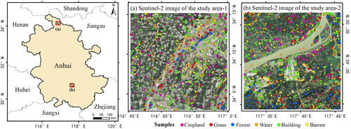
Study area 1 was located in the northern part of Anhui Province, China (Figure 1). It covers 506.25 km². The landscape is mainly plain, interspersed with low hill remnants. The cropland and residential in the study area are distributed regularly, and the water and roads are distributed in strips. In addition, Anhui Province has the greatest differences between the south and the north. The terrain and cultural differences between the north and south of Anhui are obvious due to terrain and river factors. Therefore, to ensure the diversity of the study area, study area 2 was chosen in the south of Anhui Province, with the same area of 506.25 km². The area is adjacent to the Yangtze River and has abundant water resources. The terrain is high in the south and low in the north, mainly mountains, hills, and plains in study area 2.

Figure 1. Study areas and field samples distribution.

2.2. Remote sensing imagery

The Sentinel-2 data were obtained from the Copernicus Open Access Hub (https://scihub.copernicus.eu/). They cover 13 spectral bands, from visible to short-wave infrared, and with spatial resolutions from 10 m to 60 m. In addition, Sentinel-2 images are the only optical data with three bands on the red-edge range. Therefore, they can effectively monitor vegetation information and are suitable for remote sensing image classification.

2.3. Digital elevation model (DEM) data

The DEM was obtained from NASADEM (https://lpdaac.usgs.gov/news/release-nasadem-data-products/) with a resolution of 30 m. This data is based on the Shuttle Radar Topography Mission (SRTM) data with extended coverage and improved elevation accuracy.

2.4. Field samples

According to a field survey and the USGS (United States Geological Survey) land cover classification system (Luo et al. 2021), study areas 1 and 2 included six land cover types: cropland, grass, forest, water, building, and barren. This study collected samples primarily through a field survey (collection of cropland, grass, and barren). In addition, for distinctive and easily identifiable land types, this study collected these samples through sub-metre images from Google Earth (collection of forest, water and building). All the samples were more than 10 m away from the surrounding boundary to ensure their purity. A total of 521 and 531 samples were collected in study areas 1 and 2 (Figure 1), respectively, and they were randomly divided into training and validation samples in a ratio of 7:3.

3. Methods

3.1. Extraction of single-dimensional features

As shown in Table 1, this study extracted the 12 spectral features, four texture features, and three terrain features (Yang et al. 2018; Kupidura 2019; Yang et al. 2020) based on Sentinel-2 data in study areas 1 and 2, respectively. Among the spectral features, the principal components transformed the Sentinel-2 images and selected the first principal component (PCA1, which contained more than 95% of the information) as a spectral feature. These features have the common characteristic that spectral and spatial information are separated.

Table 1. List of features.

Feature category	Specific features
spectral features	Chlorophyll Absorption Ratio Index(CARI), Ratio Vegetation Index(RVI), Differenced Vegetation Index(DVI), Enhanced Vegetation Index（EVI）, Perpendicular Vegetation Index((PVI), Normalized Difference Vegetation Index(NDVI), Soil Adjusted Vegetation Index(SAVI), Normalized Difference Vegetation Index Red-Edge3(NDVIre3), Normalized Difference Water Index(NDWI), Land Surface Water Index(LSWI), Normalized Difference Built-up Index(NDBI), PCA1
textural features	Dissimilarity, Entropy, Homogeneity, Mean
terrain features	DEM, Curvature, Slope

3.2. Extraction of spectral-spatial features

The single-dimensional features may suffer from inadequate information description. This study integrated spectral and spatial information to construct a spectral-spatial feature, namely the Pixel Neighbourhood Similarity (PNS) index. In addition, to demonstrate whether spectral-spatial features can improve classification accuracy, and which spectral-spatial feature performs better in classification. This study selected three spectral-spatial features commonly used in current studies for comparison.

3.2.1. The PNS index

According to previous studies (Kruse et al. 1993; South et al. 2004; Wan et al. 2021), the Spectral Angle Mapping（SAM）is the most representative method of projection-based spectral similarity measurement. It determines the similarity by calculating the cosine of the angle between the test spectrum and the reference spectrum. The smaller the angle, the better the match between the test spectrum and the reference spectrum.

Suppose $\mathit{A}$ and $\mathit{B}$ are two attribute vectors. The cosine between two vectors can be calculated using the Euclidean dot product formula: (1) $$\begin{array}{c}A·B=\Vert \mathit{A}\Vert \Vert \mathit{B}\Vert \cos \hspace{0.17em}\theta \end{array}$$(1) (2) $$\begin{array}{c}\cos \hspace{0.17em}\theta =\frac{\mathit{A}·\mathit{B}}{\Vert \mathit{A}\Vert \mathrm{ }\Vert \mathit{B}\Vert }=\frac{\sum _{i=1}^p{\mathit{A}}_i·{\mathit{B}}_i}{\sqrt{\sum _{i=1}^p{\left({\mathit{A}}_i\right)}^2·\sum _{i=1}^p{\left({\mathit{B}}_i\right)}^2}}\end{array}$$(2) where ${\mathit{A}}_i,$ ${\mathit{B}}_i$ represent each component of vectors $\mathit{A}$ and $\mathit{B},$ respectively. In $p$-dimensional space, the cosine similarity $\cos \hspace{0.17em}\theta$ is given by the dot product and the vector length, with values between −1 and 1.

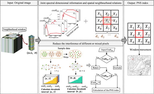
It is worth emphasising that the SAM can simultaneously use spectral information from all channels and maintain the shape difference of the spectra well. This property is important for the construction of a spectral-spatial feature. However, this method usually investigates the problem of binary spectral similarity metrics. When calculating the similarity between pixels, this metric should be converted to a multivariate metric (Zhang et al. 2022). This study implemented this conversion through neighbourhood operation. As shown in Figure 2, there are two main vital steps: (1) Joint the spectral dimensional information of pixels and the spatial neighbourhood relationships between pixels. (2) Reduce the interference of different or mixed pixels.

Figure 2. The calculation process of the PNS index.

For step (1), it is as follows:

1. A 3 × 3 template window was defined, and the cosine similarity of the centre pixel in the window to the neighbouring pixels was calculated.

2. The importance weight of pixels was assigned according to the spatial distance of the pixels in the window.

3. The average result of the window operation was assigned to the centre pixel, but the operation was based on the actual pixels in the window when the window was partially empty.

4. The window was slid in parallel, and the PNS values were assigned to all the pixels of the output image, not just the central pixel.

In addition, it is essential to note that the similarity between different land types cannot be ignored entirely. Mixed pixels or different types of pixels provide a weak dedication of similarity values to the centre pixel. This situation leads to blurred boundaries and mixed classification effects. Therefore, identifying and filtering interference pixels are also a vital problem that needs to be resolved when calculating the PNS index.

Therefore, it is necessary to establish a judgment criterion to filter out the interference pixels. In step (2), this study solved this problem based on the similarity threshold between different land types. Here, the field samples were used as a reference to calculate the similarity in the different types of samples and to find the similarity threshold β. However, it is essential to note that the permutation and combination of all samples (m × n) will produce many values before calculating β. These values need to be sufficiently pure and stable, i.e. ensure that the values are not too high (the similarity values of the different land types are not too high, actually). Therefore, this study regarded the high values as 'outliers’ and excluded them based on the similarity judgment of the same type of samples (threshold α). On this basis, the threshold β was calculated. Eventually, when constructing the PNS index, neighbouring pixels smaller than β were regarded as outliers, and their dedication to the centre pixel was reduced to 0.

In such a way, the PNS index with spectral continuity and spatial relationships was obtained. It is calculated as follows： (3) $$\begin{array}{c}PNS=\frac{1}{m}\sum _{n=1}^m\frac{R}{d_n}\frac{\sum _{k=1}^P{x}_{ik}·x_{nk}}{\sqrt{\sum _{k=1}^P{x}_{ik}^2·\sum _{k=1}^P{x}_{nk}^2}}\end{array}$$(3) where $i$ is the centre pixel with $m$ neighbouring pixels, $d_n$ is the distance of each neighbouring pixel to $i,$ and $\frac{R}{d_n}$ is the relative distance weight of each neighbouring pixel to $i.$ Here, $R$ is the spatial resolution of the images. $P$ is the number of bands, and $x_{ik}$ and $x_{nk}$ denote the value of the central pixel and its $n$ th neighbouring pixel on the $k$ th band, respectively. The closer the result is to 1, the more similar the pixel is to the neighbouring pixels, and the more likely it is to be the same type.

3.2.2. Contrast indices

These contrast features include the Vector Similarity (VS) index (Song and Yan 2014), the Change Vector Intensity (CVI) index (Bayarjargal et al. 2006), and the Correlation (COR) index calculated based on PCA1 (Qu et al. 2015).

• The VS index

VS is a detective method for spatial variation based on feature vectors. It normalized the objects involved in change detection into feature vectors ($\mathit{A}$ and $\mathit{B}$). The modulus and the angle cosine ($\cos \hspace{0.17em}\theta$) of two feature vectors were calculated to obtain the VS index. The index is calculated as follows: (4) $$\begin{array}{c}VS=\frac{\cos \hspace{0.17em}\theta }{\left|\frac{\sqrt{\sum _{i=1}^n{\left({\mathit{A}}_i\right)}^2}}{\sqrt{\sum _{i=1}^n{\left({\mathit{B}}_i\right)}^2}}-1\right|+1}\end{array}$$(4) where ${\mathit{A}}_i$ and ${\mathit{B}}_i$ represent each component of vectors $\mathit{A}$ and $\mathit{B}$ in the $n$-dimensional space, respectively.

The VS values are from 0 to 1. The closer to 1, the higher the similarity between the two vectors. The VS index and the PNS index are both cosine similarity measures, but the VS index is more complex to compute than the PNS index.

• The CVI index

CVI is a research method based on a radiometric variety of data. It determines whether the pixel type has changed by calculating the intensity of the spectral change between different pixels. The intensity of the change is expressed as Euclidean distance. The index is more commonly used for detecting spectral changes in multi-temporal. Here, this study applied it to space to detect similarities between pixels. The index is calculated as follows: (5) $$\begin{array}{c}CVI=\sqrt{{（x_{i1}-x_{j1}）}^2+{（x_{i2}-x_{j2}）}^2+\dots {（x_{ip}-x_{jp}）}^2}\end{array}$$(5) where $i$ is the centre pixel, $j$ is one of $i$'s neighbouring pixels, $p$ is the number of bands and $x$ is the value of the corresponding band.

• The COR index

The Correlation (COR) index in the Grey Level Co-occurrence Matrix (GLCM) is a spatial similarity metric. It reflects the correlation of the matrix elements in the row or column direction. However, the COR index cannot handle multidimensional spectral data simultaneously. This study extracted it based on PCA1.

3.3. Feature selection algorithm

The Correlation-based Feature Selection (CFS) algorithm is the classical filtered method based on search strategies (Hall 1998). The core of this method is using a 'Heuristic’ search strategy and a correlation assessment function to evaluate the importance of all feature combinations. The 'Heuristic’ assumes that a good feature combination contains highly correlated features with the classification targets, but features are not correlated with each other. The 'Heuristic’ calculation equation is as follows: (6) $$\begin{array}{c}{\mathit{Merit}}_s =\frac{k\overline{r_{cf}}}{\sqrt{k+k\left(k-1\right)\overline{r_{ff}}}}\end{array}$$(6) where ${\mathit{Merit}}_s$ is the 'Heuristic Merit’ of the feature combination S, the larger its value, the better the S; $k$ is the number of features contained in S; $\overline{r_{cf}}$ indicates the average correlation between features and classification targets; $\overline{r_{ff}}$ indicates the average correlation between features and features.

The CFS algorithm uses Symmetric Uncertainty (SU) to calculate the correlation of the above equation. (7) $$\begin{array}{c}SU=2*\frac{H\left(X\right)+H\left(Y\right)-H\left(X,Y\right)}{H\left(X\right)+H\left(Y\right)}\end{array}$$(7) where both $X$ and $Y$ denote sets of discrete variables containing multiple attribute values in the feature; $H\left(X\right)$ and $H\left(Y\right)$ are the 'Entropy’ of $X$ and $Y,$ respectively; $H\left(X,Y\right)$ is the joint 'Entropy’ of $X$ and $Y.$

The CFS algorithm first calculated the feature-target and feature-feature correlation matrices from the training subset. Secondly, the best first search method was used to search for features and calculated estimates for all individual features (represented by Merit values). The feature with the largest Merit value was selected into the feature combination S, and the second largest feature was selected. Suppose the Merit of these two features was less than the previous Merit. In this case, the second feature was removed, and so on, until the largest Merit combination was selected.

3.4. Assessment methods

3.4.1. Performance quality assessment of features and feature combinations

When measuring the performance quality of the PNS, VS, CVI, and COR indices from the perspective of image quality, information content and classification capability, this study chose the three indicators of Information Gain (InfoGain) (Lee C and Lee 2006), Geary’s C index (Tong et al. 2006), and ReliefF algorithm (Tan et al. 2019). The InfoGain is used to describe the ability of features to differentiate data samples and the purity of the classified attributes. The higher the value, the greater the dedication of the feature to the classification targets. The Geary’s C index is a spatial autocorrelation index. The closer its value is to 0, the more spatially informative and the higher the image quality. The larger the value, the less spatially informative it is. The ReliefF algorithm uses the 'Hypothesis Margin’ to evaluate the classification ability of features. The larger its value, the higher the quality of the feature.

Meanwhile, this study examined the performance of feature combinations from four perspectives: Dimensions (the dimensions of the combination), Merit (the Merit value of the combination), NE (the number of evaluations by the CFS algorithm), and Time (the time consumed by the combination in the classification process).

3.4.2. Accuracy assessment of classification

When evaluating the overall classification accuracy of all land types, this study selected the Overall Accuracy (OA) and the Kappa coefficient. When evaluating the extraction accuracy of each land type, the F1 score was chosen.

OA is expressed as: (8) $$\begin{array}{c}OA=\frac{\sum _{i=1}^n{p}_{i,i}}{N}\end{array}$$(8) where $p_{i,i}$ represents the total number of correctly classified land type $i,$ $n$ represents the total number of land types, and $N$ is the total number of samples.

Kappa is expressed as: (9) $$\begin{array}{c}K\mathit{appa}=\frac{N^2\mathrm{*}OA-\sum _{i=1}^n{a}_i{b}_i}{N^2-\sum _{i=1}^n{a}_i{b}_i}\end{array}$$(9) where $a_i$ is the number of actual samples in each land type, and $b_i$ is the number of predicted samples in each land type.

When evaluating the extraction accuracy of each land type, this study classified the pixels into four types: correctly identified as this class, correctly identified as other class, incorrectly identified as this class, and incorrectly identified as other class. They were represented by True Positives (TP), True Negatives (TN), False Positives (FP), and False Negatives (FN), respectively. The F1 score is the harmonic average of the Precision and Recall. Precision and Recall are defined as: (10) $$\begin{array}{c}P\mathit{recision}=\frac{TP}{TP+FP}\end{array}$$(10) (11) $$\begin{array}{c}R\mathit{ecall}=\frac{TP}{TP+FN}\end{array}$$(11)

The F1 score is expressed as: (12) $$\begin{array}{c}F1=\frac{2P\mathit{recision}\mathrm{*}\mathit{Recall}}{\mathit{Precision}+\mathit{Recall}}\end{array}$$(12)

4. Experiments

4.1. Determine the similarity thresholds α, β in the PNS index

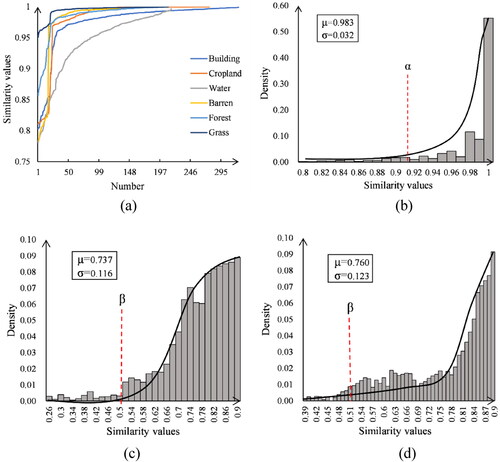
In the similarity threshold experiment, some different types of samples were more similar. Therefore, according to the flow in Figure 2, these outliers need to be filtered by the similarity threshold α. Due to the values were distributed stably (Figure 3a) and presented a half-normal distribution (Figure 3b) in the same type of samples. In this case, this study set a confidence level of 0.95 by trial and error. From the mean (μ) and standard deviation (σ), the threshold α was 0.919 and 0.893 in study areas 1 and 2, respectively. After excluding outliers higher than α, the remaining values also showed a half-normal distribution (Figure 3c and 3d). Therefore, the threshold β was still calculated at the confidence level of 0.95 and was 0.505 and 0.514 in study areas 1 and 2, respectively. Ultimately, the neighbourhood pixels with similarity values less than 0.505 and 0.514 were treated as different types from the centre pixel and ignored their values when constructing the PNS index.

Figure 3. Distribution of similarity values for the samples. (a) Similarity values and (b) half-normal distribution for the same type of samples in study area 1, and half-normal distribution for the different types of samples in (c) study area 1, and (d) study area 2.

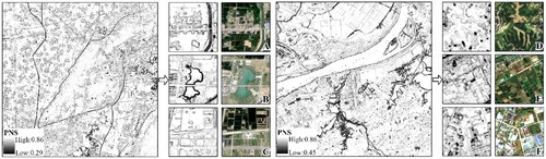
The PNS index is shown in Figure 4. Six sub-areas (A-F) in study areas 1 and 2 were randomly selected for image presentation. The values were relatively high within the same land type and low at the boundaries of different land types. For example, the cropland in patches with high and homogeneous values. The building and water with clear and continuous boundaries. The results show that the PNS index can highlight the boundaries of land cover types.

Figure 4. Detailed display of the PNS index.

4.2. Feature combination schemes

The 19 single-dimensional features in Table 1 were involved in the CFS algorithm, resulting in a single-dimensional combination (SIN-CFS). The four spectral-spatial features (PNS, VS, CVI, and COR) were separately involved in the CFS algorithm with single-dimensional features, resulting in the corresponding feature combinations: PNS-CFS, VS-CFS, CVI-COM, and COR-COM. Among them, the CVI and COR indices were filtered out in the experiment, but as the contrast indices for PNS, this study combined the remaining features in the PNS-CFS except for the PNS index with CVI and COR to form CVI-COM and COR-COM, respectively. The features contained in SIN-CFS, PNS-CFS, VS-CFS, CVI-COM and COR-COM are shown in Table 2. PNS-CFS reduced three dimensions and one dimension compared to SIN-CFS in study areas 1 and 2. This indicates that adding the PNS index to the CFS algorithm can effectively reduce the dimension of the combination.

Table 2. List of features of the four combination schemes.

Study areas	Feature combinations	Features
1	SIN -CFS	NDVIre3, NDWI, LSWI, CARI, DVI, RVI, Mean, DEM, Slope, DIS, NDBI, PVI
	PNS-CFS	NDVIre3, NDWI, LSWI, CARI, DVI, RVI, Mean, DEM, PNS
	VS-CFS	NDVIre3, NDWI, LSWI, CARI, RVI, DEM, DVI, Mean, VS, HOM, PVI
	CVI-COM	NDVIre3, NDWI, LSWI, CARI, DVI, RVI, Mean, DEM, CVI
	COR-COM	NDVIre3, NDWI, LSWI, CARI, DVI, RVI, Mean, DEM, COR
2	SIN -CFS	NDVIre3, NDWI, LSWI, CARI, RVI, EVI, DEM, PCA1, PVI, DIS
	PNS-CFS	NDVIre3, NDWI, LSWI, CARI, RVI, EVI, DEM, PCA1, PNS
	VS-CFS	NDVIre3, NDWI, LSWI, CARI, RVI, DEM, EVI, PCA1, VS, PVI
	CVI-COM	NDVIre3, NDWI, LSWI, CARI, RVI, EVI, DEM, PCA1, CVI
	COR-COM	NDVIre3, NDWI, LSWI, CARI, RVI, EVI, DEM, PCA1, COR

5. Results

5.1. Feature space analysis

For the spatial analysis of features, this study analysed the importance of features, the separation of features to land types and the correlation between features. When analysing the importance of features, the Merit values of each feature are shown in Table 3. It can be seen that the Merit values were relatively high on the spectral features and relatively low on the terrain and texture features. In addition, the Merit values of the spectral-spatial features were ranked from high to low in study area 1 as PNS > VS > CVI > COR and in study area 2 as PNS > CVI > VS > COR. In comparison, the PNS index performed better. Moreover, this study further explored the separation of features to land types and selected the PNS, VS, CVI, and COR indices and the other five features with high Merit values (NDWI, LSWI, CARI, Mean, and DEM) for analysis. As shown in Figure 5, for NDWI, LSWI, CARI, and Mean, the six land types showed a favourable gradient distribution, and the average of each type was highly variable. In contrast, for the PNS, VS, CVI, and DEM, their values were relatively concentrated and had poor separability for land types. For example, grass, forest, and barren are irregularly distributed in study areas, so they had a high span in DEM. Cropland, water, and building are primarily associated with human activity, so their elevations were low and concentrated in DEM. Likewise, the PNS index reflects the similarity between land types, and the values were almost identical within each land type. It also showed a concentrated distribution of values. Therefore, these features not only reflected their ability to separate land types, but also reflected the distribution characteristics of land types.

Figure 5. The ability of features to separate land types. The centerline of each box in the boxplot is the median, and the edges of the box represent the upper and lower quartiles.

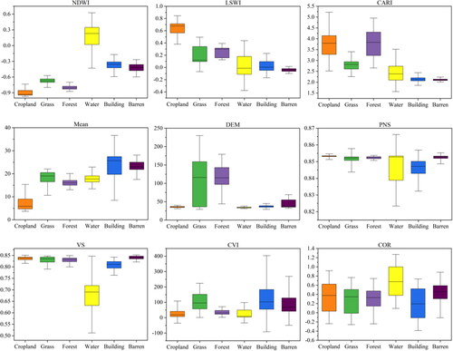
Table 3. Merit values of all features in the classification.

Study area 1				Study area 2
Features	Merit	Features	Merit	Features	Merit	Features	Merit
DVI	0.58	NDBI	0.40	NDWI	0.52	NDVIre3	0.31
NDWI	0.57	VS	0.31	RVI	0.51	PNS	0.26
RVI	0.57	DEM	0.26	SAVI	0.51	CVI	0.23
SAVI	0.57	Slope	0.25	NDVI	0.51	VS	0.20
NDVI	0.57	NDVIre3	0.20	PVI	0.44	DEM	0.20
PVI	0.57	CVI	0.15	DVI	0.43	DIS	0.19
MEAN	0.47	HOM	0.09	CARI	0.42	HOM	0.17
PCA1	0.44	DIS	0.09	NDBI	0.42	COR	0.13
PNS	0.41	ENT	0.08	LSWI	0.42	ENT	0.13
LSWI	0.41	COR	0.01	PCA1	0.36	Slope	0.09
CARI	0.41	CUR	0.01	MEAN	0.35	CUR	0.01

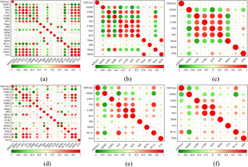
When exploring the correlation between features, this study compared feature correlation in all features, SIN-CFS, and PNS-CFS, to explore whether feature selection and spectral-spatial features reduce feature redundancy. As shown in Figure 6, the feature pairs with high correlation (Pearson correlation coefficient ≥ 0.8 or ≤ −0.8) of all features, SIN-CFS and PNS-CFS were 18.42%, 13.64% and 8.33% in study area 1 and 10.00%, 6.67% and 2.78% in study area 2, respectively. The ratios became significantly smaller, and PNS-CFS had the lowest correlation between features. Therefore, feature selection can reduce the correlation between features compared to all features, and adding the PNS Index in feature selection can significantly reduce the correlation compared to SIN-CFS.

Figure 6. Correlation between features. From (a) to (c), represent all features, SIN-CFS, and PNS-CFS in study area 1, respectively, and from (d) to (f), represent all features, SIN-CFS, and PNS-CFS in study area 2.

5.2. Performance quality of features and feature combinations

When measuring the quality of spectral-spatial features (Table 4), the PNS index had the highest InfoGain and ReliefF values in study areas 1 and 2, indicating that the PNS has information and the ability to differentiate land types. However, the VS and COR indices had Geary’s C of 0.88 and 0.98 in study areas 1 and 2, respectively, and they performed relatively best. Geary’s C of the PNS index was intermediate, which may be related to the fragmentation phenomenon and distribution characteristics of land types. Overall, from the perspective of InfoGain, Geary’s C, and ReliefF, it can be concluded that the PNS index has high reliability.

Table 4. Quality of the PNS, VS, CVI, and COR indices.

Study areas	Metric indicators	PNS	VS	CVI	COR
1	InfoGain	0.86	0.59	0.27	0.74
	Geary’s C	0.92	0.88	0.95	0.95
	ReliefF	0.04	0.03	0.02	0.01
2	InfoGain	0.61	0.44	0.56	0.22
	Geary’s C	1.03	1.02	1.04	0.98
	ReliefF	0.04	0.04	0.02	0.03

When assessing the performance of the feature combinations (Table 5), the Dimensions, NE, and Time (Time calculated based on the ENVI5.3 platform IDL8.5 with 2.6 GHz Intel i7-6700HQ CPU and 8 GB RAM) of the PNS-CFS were relatively low, and the Merit values were relatively highest. By comparison, it can be concluded that the PNS-CFS has the best performance.

Table 5. Performance of SIN-CFS, PNS-CFS, VS-CFS, CVI-COM, COR-COM.

Study areas	Metric indicators	SIN-CFS	PNS-CFS	VS-CFS	CVI-COM	COR-COM
1	Dimensions	12	9	11	9	9
	Merit	0.71	0.74	0.73	<0.71	<0.71
	NE	210	203	208	/	/
	Time(s)	192	131	138	137	132
2	Dimensions	10	9	10	9	9
	Merit	0.67	0.68	0.68	<0.67	<0.67
	NE	204	195	200	/	/
	Time(s)	161	115	123	115	109

Note: CVI-COM and COR-COM combined features from PNS-CFS other than PNS and were not directly involved in the CFS algorithm. Therefore, they do not contain NE and Merit is an estimation interval.

5.3. Classification results and accuracy assessment of feature combinations

5.3.1. Classification results

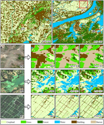
In order to explore the effects before and after adding the PNS index to the CFS algorithm, this paper compared the classification results of SIN-CFS, PNS-CFS, and the original images (ORI). As shown in Figure 7, a Random Forest algorithm (Breiman 2001) was used for classification, and three sub-areas were selected for presentation. The ORI had relatively poor identification for barren. In contrast, the SIN-CFS and PNS-CFS maintained the integrity of the barren very well. Moreover, the PNS-CFS maintained better continuity for narrow roads than the SIN-CFS.

Figure 7. Classification results for ORI, SIN-CFS, and PNS-CFS.

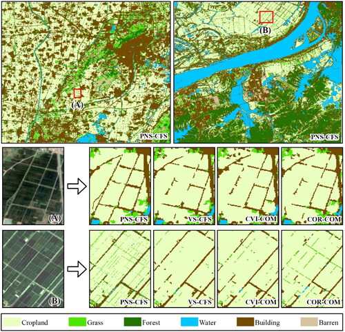
Meanwhile, to compare the classification results of the spectral-spatial features (PNS, VS, CVI, and COR), this study compared their combinations: PNS-CFS, VS-CFS, CVI-COM, and COR-COM (Figure 8). For narrower roads, the PNS-CFS performed best than others. It kept the continuity of roads very well. Likewise, for the finer areas between fields, PNS-CFS extracted them as grass and maintained good line properties. However, VS-CFS and CVI-COM still identified them as cropland. COR-COM had a good identification only for these wider areas. In general, the PNS-CFS better maintained the continuity and integrity of land types. This is mainly related to the fact that the PNS index enhances the differentiation boundaries of the land types.

Figure 8. Classification results for PNS-CFS, VS-CFS, CVI-COM, and PC-COM.

5.3.2. Accuracy assessment

The classification accuracy of all feature combinations was assessed in Table 6. The OA and Kappa were ranked from high to low in study area 1 as PNS-CFS > VS-CFS > CVI-COM > SIN-CFS > ORI > COR-COM and in study area 2 as PNS-CFS > VS-CFS > CVI-COM > SIN-CFS > COR-COM > ORI. The classification accuracy of PNS-CFS was the highest. The OA of PNS-CFS was 94.66% and 93.59% in study areas 1 and 2, respectively. This was 7.48% and 6.02% higher than ORI, respectively. Likewise, this was 7.27% and 2.39% higher than SIN-CFS, respectively. Furthermore, when comparing the F1 scores for each land type (Table 7), grass, forest, and building had relatively better F1 scores in PNS-CFS and VS-CFS. Water and barren had the best F1 scores in COR-COM and PNS-CFS, respectively. The F1 scores of the cropland were better in the ORI and VS-CFS in study area 1, and PNS-CFS and VS-CFS were better in study area 2. In general, the F1 scores of all land types were relatively stable and high in PNS-CFS and reached over 82%. This was mainly related to the PNS index can enhance the differences between land types and improve the boundaries of distinction between them. Not only that, Figure 9 shows a confusion matrix (with study area 2 as an example). It was used to deeply analyse the feature combinations to extract information about the land types. Each land type was more or less misclassified as building or cropland in all combinations. For example, ORI, VS-CFS, and CVI-COM misclassified 12%, 10%, and 11% of grass as building, respectively. ORI misclassified 13% of forest as cropland. Likewise, 10% of grass and barren was misclassified as cropland and building by COR-COM. These rates of misclassification were relatively high, at around 10%. It is worth noting that PNS-CFS kept the misclassification rate to less than 6% for each land type. Moreover, PNS-CFS improved the extraction accuracy of all land types compared to ORI and SIN-CFS (the extraction accuracy of waters was relatively flat). It also improved the accurate rate of grass, forest, building and barren compared to VS-CFS, CVI-COM, and COR-COM. Among them, the accurate rate of grass and building increased the most. It increased by 4%–13% and 2%–15%, respectively. Therefore, PNS-CFS was superior to other feature combinations.

Figure 9. Confusion matrix of classification results for each land type based on different feature combinations.

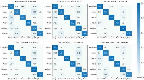
Table 6. The OA and Kappa for feature combinations.

Study areas	Accuracy	ORI	SIN-CFS	PNS-CFS	VS-CFS	CVI-COM	COR-COM
1	OA /(%)	87.18	87.39	94.66	92.52	88.46	86.75
	Kappa	0.84	0.84	0.93	0.91	0.86	0.83
2	OA/(%)	87.57	91.20	93.59	92.74	91.40	90.48
	Kappa	0.83	0.88	0.92	0.90	0.89	0.87

Table 7. The F1 score for each land type.

Study areas	Land types	ORI	SIN-CFS	PNS-CFS	VS-CFS	CVI-COM	COR-COM
1	Cropland	95.65	94.11	94.89	94.97	94.20	93.85
	Grass	95.00	93.55	96.00	100.00	99.17	89.23
	Forest	90.00	91.93	94.12	90.76	90.76	88.52
	Water	95.83	94.36	97.26	97.96	97.26	100.00
	Building	87.85	86.77	95.36	91.67	86.17	78.41
	Barren	48.28	51.77	87.85	76.77	57.45	80.65
2	Cropland	62.32	72.27	82.13	80.55	79.54	72.68
	Grass	69.36	77.58	89.14	85.72	80.66	73.94
	Forest	91.13	94.65	96.74	97.36	96.46	95.07
	Water	94.89	95.65	95.23	94.58	94.74	95.83
	Building	84.67	87.90	91.25	89.33	85.58	85.66
	Barren	88.07	93.12	95.98	95.62	93.11	89.57

6. Discussion

6.1. Analysis of spectral-spatial features

For the spectral-spatial features, this study constructed the PNS index and three contrast indices (VS, CVI, and COR). Among them, spectral and spatial information were considered simultaneously in the PNS, VS, and CVI indices. The COR index separated the spectral and spatial information when it was constructed. Firstly, it compressed the spectral information into a one-dimensional plane and then extracted the spatial features. However, Zhang et al. (2018) proved the superiority of simultaneously combining spectral and spatial information when constructing spectral-spatial features. Their point also was demonstrated in this study. This is because the COR index had poor performance quality (Table 4) and classification accuracy (Table 6).

In addition, the PNS and VS indices were based on cosine similarity, unlike the CVI index. The cosine similarity distinguishes the difference from the direction. It reflects relative differences in values and is not sensitive to absolute values. Even in high-dimensional data, the cosine similarity remains between 0 and 1. In contrast, the CVI index was based on Euclidean distance. Euclidean distance reflects the absolute difference in values. This characteristic causes the values to be susceptible to dimensionality, and the range of values is unstable. In classification studies, the spectral values are not uniform and are impossibly distributed in the same range due to the different types of pixels. Therefore, when measuring whether pixels are similar, more attention is paid to the relative differences in pixels, and the PNS and VS indices possess this property. In comparative experiments on performance and accuracy, it is easy to find that the PNS and VS indices performed better. However, the VS index had a relatively high computational complexity. In Table 5, the quality assessment of the VS index was relatively lower than the PNS index. In this study, the PNS index considered the spectral information, spatial relationships, and distance proximity of the pixels simultaneously. It also contained the judgement criterion of similarity, which can effectively filter out interfering pixels, highlight the boundaries of land types (Figure 6) and amplify the differences between land types.

6.2. Analysis of feature combinations

The performance quality and classification accuracy of PNS-CFS was relatively highest through the multiple region experiments and the comparisons. PNS-CFS made the extraction results of land types present a high continuity and integrity (Figures 7 and 8). In study areas 1 and 2, the OA of PNS-CFS was 7.48% and 6.02% higher than ORI and 7.27%, and 2.39% higher than SIN-CFS, respectively. PNS-CFS significantly improved classification accuracy. Moreover, this study only used the CFS algorithm to feature selection. It is mainly considered that this algorithm can return the features as a combination, which is more convenient when constructing feature combinations. Although the CFS algorithm achieved good results in feature selection, different algorithms are suitable for different scenarios, and no uniform conclusion has been formed yet. Other algorithms such as Factor Analysis (Kondratyev and Pokrovsky 1979), SeaTH algorithm (Vanniel et al. 2005), Gain Ratio (Jeppson 1994), Optimum Index Factor (Chavez et al. 1982). Alternatively, some improved algorithms based on PCA. Such as Folded-PCA (FPCA), Spectrally-Segmented-FPCA (SSFPCA) and Segmented-FPCA (SFPCA) (Xiuping and Richards 1999; Uddin et al. 2019, 2021b). These methods can also be considered in feature selection. In general, the PNS index and the CFS algorithm in this study are only used as a reference.

6.3. Performance of the datasets and classification algorithms for extracting land types

The Sentinel-2 can provide multispectral images with a short replay period, high spatial resolution, and global coverage. In addition, hyperspectral images also have been widely used in classification studies (Rastogi et al. 2022). Compared to multispectral data, it has near-continuous spectral information, which significantly improves the detection and identification of land types. However, when extracting features based on hyperspectral data, the data must be reduced in dimension, which inevitably increases the computational effort. For the extraction of spectral-spatial features, both spectral and spatial information need to be considered. Although hyperspectral data has massive spectra, this advantage results in relatively low spatial resolution. In large-scale classification studies, open and timely data often helps strengthen land planning and management decisions.

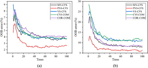
For the classification algorithm, this study used the random forest algorithm. This algorithm uses a parallel approach to construct decision trees, and each tree is constructed using independent samples from the training set. Limited and unusual samples have less impact on the results. Moreover, The Out-Of-Bag (OOB) error can measure the classification accuracy of the random forest (Zhu et al. 2019b). This study used OOB error to measure the classification effect of different feature combinations (Figure 10). In the figure, the OOB error of PNS-CFS was always the smallest compared to the other combinations. This also proved that random forest had the highest classification accuracy in the PNS-CFS. In addition, the deep neural network (DNN) algorithm has also been widely used for classification problems (Cai et al. 2018). However, in this study, the sample sizes in the hundreds did not satisfy the criteria of DNN, and large area classification also affected the classification efficiency of DNN. In the future, deep learning methods will be used to promote the ability of image classification.

Figure 10. The OOB error for different feature combinations in (a) study area 1, and (b) study area 2.

7. Conclusions

This study proposed a combination of spatial-spectral features (PNS-CFS) to classify images. This combination achieved accurate classification and produced reliable results in different study areas. With the following conclusions:

1. The PNS index had high and homogeneous values in the same land cover type and low values in the boundary areas of different land cover types. This characteristic make objects with obvious boundaries.

2. In study areas 1 and 2, the PNS-CFS reduced the high-correlated feature pairs by 10.09% and 7.22%, respectively, compared to all features without feature selection. Compared to the single-dimensional feature combination (SIN-CFS), it decreased by 5.31% and 3.89%, respectively. PNS-CFS significantly reduced the correlation between features. When comparing the quality of the features, the InfoGain, Geary’s C and ReliefF values of the PNS index were relatively best. The performance of PNS-CFS was also relatively optimal when comparing the performance quality of the feature combinations.

3. The overall accuracy (OA) of the PNS-CFS was 94.66% and 93.59% in study areas 1 and 2, respectively. This result is 7.27% and 2.39% higher than the combination without the PNS index (SIN-CFS), and 7.48% and 6.02% higher than the original images (ORI).

These results demonstrated that the PNS index is a superior spectral-spatial feature, and the PNS-CFS is a feature combination with high performance and classification accuracy. When classifying images from the perspective of feature extraction, the construction approach of the PNS index and the PNS-CFS can provide an idea.

Acknowledgments

The authors would like to thank the anonymous reviewers for their valuable comments to improve the quality of the paper. We thank the teachers and classmates for their technical help.

Disclosure statement

No potential conflict of interest was reported by the authors.

Additional information

Funding

This work was supported by the National Natural Science Foundation of China (41201408), and the Zhejiang Provincial Natural Science Foundation of China (LY16D010009).

References

- Bayarjargal Y, Karnieli A, Bayasgalan M, Khudulmur S, Gandush C, Tucker C. 2006. A comparative study of NOAA–AVHRR derived drought indices using change vector analysis. Remote Sens Environ. 105(1):9–22.
- Ben Brick AS, Laroussi N, Mesrati H, Kefi R, Bchetnia M, Lasram K, Ben Halim N, Romdhane L, Ouragini H, Marrakchi S, et al. 2014. Mutational founder effect in recessive dystrophic epidermolysis bullosa families from Southern Tunisia. Arch Dermatol Res. 306(4):405–411.
- Benediktsson JA, Pesaresi M, Arnason K. 2003. Classification and feature extraction for remote sensing images from urban areas based on morphological transformations. IEEE Trans Geosci Remote Sens. 41(9):1940–1949.
- Bolourchi P, Demirel H, Uysal S. 2018. Entropy‐score‐based feature selection for moment‐based SAR image classification. Electron Lett. 54(9):593–595.
- Breiman L. 2001. Random forests. Mach Learn. 45(1):5–32.
- Cai Y, Guan K, Peng J, Wang S, Seifert C, Wardlow B, Li Z. 2018. A high-performance and in-season classification system of field-level crop types using time-series Landsat data and a machine learning approach. Remote Sens Environ. 210:35–47.
- Chavez PS, Berlin GL, Sower LB. 1982. Statistical method for selecting Landsat MSS ratios. J Appl Photogr Eng. 8(1):23–30.
- Chen N, Yu L, Zhang X, Shen Y, Zeng L, Hu Q, Niyogi D. 2020. Mapping paddy rice fields by combining multi-temporal vegetation index and synthetic aperture radar remote sensing data using Google Earth Engine machine learning platform. Remote Sens. 12(18):2992–3008.
- Chen Y, He X, Xu J, Zhang R, Lu Y. 2020. Scattering feature set optimization and polarimetric SAR classification using object-oriented RF-SFS algorithm in coastal Wetlands. Remote Sens. 12(3):407–423.
- Chen Y, Luo Z, Kong L. 2021. ℓ2,0-norm based selection and estimation for multivariate generalized linear models. J Multivariate Anal. 185:104782–104799.
- Du Q. 2007. Modified Fisher’s linear discriminant analysis for hyperspectral imagery. IEEE Geosci Remote Sens Lett. 4(4):503–507.
- Duan L, Yang S, Zhang D. 2020. The optimization of feature selection based on chaos clustering strategy and niche particle swarm optimization. Math Prob Eng. 2020:1–8.
- Freeman C, Kulić D, Basir O. 2015. An evaluation of classifier-specific filter measure performance for feature selection. Pattern Recognit. 48(5):1812–1826.
- Haralick RM, Shanmugam K, Dinstein I. 1973. Textural features for image classification. IEEE Trans Syst Man Cybern. SMC-3(6):610–621.
- Hua Y, Wang X, Li Y, Xu P, Xia W. 2021. Dynamic development of landslide susceptibility based on slope unit and deep neural networks. Landslides. 18(1):281–302.
- Huang X, Zhang L. 2008. An adaptive mean-shift analysis approach for object extraction and classification from urban hyperspectral imagery. IEEE Trans Geosci Remote Sens. 46(12):4173–4185.
- Imani M, Ghassemian H. 2015. Feature extraction using median–mean and feature line embedding. Int J Remote Sens. 36(17):4297–4314.
- Immitzer M, Neuwirth M, Böck S, Brenner H, Vuolo F, Atzberger C. 2019. Optimal input features for tree species classification in central Europe based on multi-temporal sentinel-2 data. Remote Sens. 11(22):2599–2621.
- Jeppson KO. 1994. Modeling the influence of the transistor gain ratio and the input-to-output coupling capacitance on the CMOS inverter delay. IEEE J Solid-State Circuits. 29(6):646–654.
- Kondratyev KY, Pokrovsky OM. 1979. A factor analysis approach to optimal selection of spectral intervals for multipurpose experiments in remote sensing of the environment and earth resources. Remote Sens Environ. 8(1):3–10.
- Kruse FA, Lefkoff AB, Boardman JW, Heidebrecht KB, Shapiro AT, Barloon PJ, Goetz AFH. 1993. The spectral image processing system (SIPS)—interactive visualization and analysis of imaging spectrometer data. Remote Sens Environ. 44(2–3):145–163.
- Kupidura P. 2019. The comparison of different methods of texture analysis for their efficacy for land use classification in satellite imagery. Remote Sens. 11(10):1233–1253.
- Lee C, Lee GG. 2006. Information gain and divergence-based feature selection for machine learning-based text categorization. Inf Process Manag. 42(1):155–165.
- Lee J, Kim D-W. 2015. Memetic feature selection algorithm for multi-label classification. Inf Sci. 293:80–96.
- Li LH, Jia XM, Zhang JT. 2014. Research on extraction and assistant classification of remote sensing for texture feature. AMR. 1073–1076:1881–1885.
- Li Z, Zhu Q, Wang Y, Zhang Z, Zhou X, Lin A, Fan J. 2020. Feature extraction method based on spectral dimensional edge preservation filtering for hyperspectral image classification. Int J Remote Sens. 41(1):90–113.
- Luo X, Du H, Zhou G, Li X, Mao F, Zhu D, Xu Y, Zhang M, He S, Huang Z. 2021. A novel query strategy-based rank batch-mode active learning method for high-resolution remote sensing image classification. Remote Sens. 13(11):2234.
- Prasad S, Bruce LM. 2008. Limitations of principal components analysis for hyperspectral target recognition. IEEE Geosci Remote Sens Lett. 5(4):625–629.
- Qian Y, Ye M, Zhou J. 2013. Hyperspectral image classification based on structured sparse logistic regression and three-dimensional wavelet texture features. IEEE Trans Geosci Remote Sens. 51(4):2276–2291.
- Qu J-H, Cheng J-H, Sun D-W, Pu H, Wang Q-J, Ma J. 2015. Discrimination of shelled shrimp (Metapenaeus ensis) among fresh, frozen-thawed and cold-stored by hyperspectral imaging technique. LWT - Food Sci Technol. 62(1):202–209.
- Rastogi K, Bodani P, Sharma SA. 2022. Automatic building footprint extraction from very high-resolution imagery using deep learning techniques. Geocarto Int. 37(5):1501–1513.
- Saha S, Rajasekaran S, Ramprasad R. 2015. Novel randomized feature selection algorithms. Int J Found Comput Sci. 26(03):321–341.
- Shukla AK, Singh P, Vardhan M. 2019. A new hybrid wrapper TLBO and SA with SVM approach for gene expression data. Inf Sci. 503:238–254.
- Sitokonstantinou V, Papoutsis I, Kontoes C, Arnal A, Andrés AP, Zurbano JA. 2018. Scalable parcel-based crop identification scheme using sentinel-2 data time-series for the monitoring of the Common Agricultural Policy. Remote Sens. 10(6):911–931.
- Song X, Yan C. 2014. Land cover change detection using segment similarity of spectrum vector based on knowledge base. Acta Ecol Sinica. 34(24):7175–7180.
- Sonnenschein R, Kuemmerle T, Udelhoven T, Stellmes M, Hostert P. 2011. Differences in Landsat-based trend analyses in drylands due to the choice of vegetation estimate. Remote Sens Environ. 115(6):1408–1420.
- South S, Qi J, Lusch DP. 2004. Optimal classification methods for mapping agricultural tillage practices. Remote Sens Environ. 91(1):90–97.
- Taghizadeh-Mehrjardi R, Toomanian N, Khavaninzadeh AR, Jafari A, Triantafilis J. 2016. Predicting and mapping of soil particle-size fractions with adaptive neuro-fuzzy inference and ant colony optimization in central Iran. Eur J Soil Sci. 67(6):707–725.
- Tan C, Chen H, Lin Z, Wu T. 2019. Category identification of textile fibers based on near-infrared spectroscopy combined with data description algorithms. Vib Spectrosc. 100:71–78.
- Tong QX, Zhang B, Zheng FL. 2006. Hyperspectral remote sensing. Beijing, China: higher Education Press.
- Toure SI, Stow DA, Shih H-c, Weeks J, Lopez-Carr D. 2018. Land cover and land use change analysis using multi-spatial resolution data and object-based image analysis. Remote Sens Environ. 210:259–268.
- Uddin MP, Mamun MA, Afjal MI, Hossain MA. 2021a. Information-theoretic feature selection with segmentation-based folded principal component analysis (PCA) for hyperspectral image classification. Int J Remote Sens. 42(1):286–321.
- Uddin MP, Mamun MA, Hossain MA. 2019. Effective feature extraction through segmentation-based folded-PCA for hyperspectral image classification. Int J Remote Sens. 40(18):7190–7220.
- Uddin MP, Mamun MA, Hossain MA. 2021b. PCA-based feature reduction for hyperspectral remote sensing image classification. IETE Tech Rev. 38(4):377–396.
- Vanniel T, McVicar T, Datt B. 2005. On the relationship between training sample size and data dimensionality: monte Carlo analysis of broadband multi-temporal classification. Remote Sens Environ. 98(4):468–480.
- Villa A, Benediktsson JA, Chanussot J, Jutten C. 2011. Hyperspectral image classification with independent component discriminant analysis. IEEE Trans Geosci Remote Sens. 49(12):4865–4876.
- Wan Y, Ma A, Zhang L, Zhong Y. 2021. Multiobjective sine cosine algorithm for remote sensing image spatial-spectral clustering. p. 1–15.
- Wu B, Chen C, Kechadi TM, Sun L. 2013. A comparative evaluation of filter-based feature selection methods for hyper-spectral band selection. Int J Remote Sens. 34(22):7974–7990.
- Xiuping Jia M, Richards JA. 1999. Segmented principal components transformation for efficient hyperspectral remote-sensing image display and classification. IEEE Trans Geosci Remote Sens. 37(1):538–542.
- Xu Y, Wang J, Xia A, Zhang K, Dong X, Wu K, Wu G. 2019. Continuous wavelet analysis of leaf reflectance improves classification accuracy of mangrove species. Remote Sens. 11(3):254–270.
- Yang S, Gu L, Li X, Jiang T, Ren R. 2020. Crop classification method based on optimal feature selection and hybrid CNN-RF networks for multi-temporal remote sensing imagery. Remote Sens. 12(19):3119–3142.
- Yang X, Qin Q, Grussenmeyer P, Koehl M. 2018. Urban surface water body detection with suppressed built-up noise based on water indices from Sentinel-2 MSI imagery. Remote Sens Environ. 219:259–270.
- Zhang L,Zhang Q,Du B,Huang X,Tang YY,Tao D. 2018. Simultaneous spectral-spatial feature selection and extraction for hyperspectral images. IEEE Trans Cybern. 48(1):16–28.
- Zhang K, Chen Y, Zhang B, Hu J, Wang W. 2022. A multitemporal mountain rice identification and extraction method based on the optimal feature combination and machine learning. Remote Sens. 14(20):5096.
- Zhang L, Zhu X, Zhang L, Du B. 2016. Multidomain subspace classification for hyperspectral images. IEEE Trans Geosci Remote Sens. 54(10):6138–6150.
- Zhang P, He H, Gao L. 2019. A nonlinear and explicit framework of supervised manifold-feature extraction for hyperspectral image classification. Neurocomputing. 337:315–324.
- Zhao J, Fang Y, Zhang M, Dong Y. 2020. Identification of remote sensing-based land cover types combining nearest-neighbor classification and SEaTH algorithm. J Indian Soc Remote Sens. 48(7):1007–1020.
- Zhao W, Du S. 2016. Spectral–spatial feature extraction for hyperspectral image classification: a dimension reduction and deep learning approach. IEEE Trans Geosci Remote Sens. 54(8):4544–4554.
- Zhou Q, Zhou H, Li T. 2016. Cost-sensitive feature selection using random forest: selecting low-cost subsets of informative features. Knowl-Based Syst. 95:1–11.
- Zhu J, Pan Z, Wang H, Huang P, Sun J, Qin F, Liu Z. 2019a. An improved multi-temporal and multi-feature tea plantation identification method using sentinel-2 imagery. Sensor. 19(9):2087–2103.
- Zhu J, Pan Z, Wang H, Huang P, Sun J, Qin F, Liu Z. 2019b. An improved multi-temporal and multi-feature tea plantation identification method using sentinel-2 imagery. Sensors (Basel). 19(9):2087.
- Zhu Z, Jia S, He S, Sun Y, Ji Z, Shen L. 2015. Three-dimensional Gabor feature extraction for hyperspectral imagery classification using a memetic framework. Inf Sci. 298:274–287.