Development of chlorophyll-a concentration estimation algorithm for turbid productive inland waters in India

Abstract

Estimation of Chlorophyll-a (Chl-a) concentration from remote-sensing reflectance derived from satellite imagery is highly effective in monitoring the spatial and temporal optical variations in water bodies. In turbid, productive and inland waters, implementation of traditional Chl-a estimation algorithms using the blue and green wavelength bands results in higher error in estimated Chl-a. To minimize the absorption and scattering effects of other water constituents like colored dissolved organic matter and particulate matter, the wavelengths bands in red and Near Infrared (NIR) are generally used for estimating Chl-a concentration in productive waters. Owing to a widely observed optical variability in natural waters, a single universal algorithm is not applicable to all waterbodies, hence, regional tuning of algorithms is necessary for estimating Chl-a in turbid and inland productive waters. Here, a 2-band based algorithm of the form $R_{rs}({\lambda }_1)/R_{rs}({\lambda }_2)$ and a 3-band algorithm of form $\left[R_{rs}^{-1}\left({\lambda }_1\right)-R_{rs}^{-1}\left({\lambda }_2\right)\right] \times R_{rs}\left({\lambda }_3\right)$ were tuned for Chl-a estimation based on field measurements carried out in three water bodies, Chilika Lake of Orissa, Ujjani Reservoir of Maharashtra, Vallabh Sagar Reservoir of Gujarat, India, wherein the observed Chl-a concentration range is 5–33 mg/m³. Together with measured in situ reflectance spectra and concurrent Chl-a concentrations, tuning of red-NIR algorithms is performed. The optimal wavelengths to estimate Chl-a found by the proximal sensing method are ${\lambda }_1$ = 691 nm and ${\lambda }_2$ = 667 nm in case of 2-band red-NIR type algorithm. For 3-band red-NIR algorithm, the optimal wavelengths are ${\lambda }_1$ = 670 nm, ${\lambda }_2$ = 696 nm and ${\lambda }_3$ = 740 nm. The mean absolute percentage error (MAPE) and root-mean-square error (RMSE) values obtained for the estimated Chl-a using the tuned 2-band red-NIR algorithm are 29.9% and 5.35 $\mathrm{mg}/{\mathrm{m}}^3,$ respectively. Similarly, RMSE and MAPE values for Chl-a concentration estimated using the 3-band tuned red-NIR algorithm are 4.24 $\mathrm{mg}/{\mathrm{m}}^3$ and 22.5%, respectively. The tuned 2-band and 3-band algorithms resulted in better Chl-a estimates than the fourteen blue-green and red-NIR algorithms from previous studies. The 2-band and 3-band algorithms were re-calibrated to wavelengths present in the ocean land color imager (OLCI) sensor on Sentinel-3 satellite to monitor these water bodies. Spatio-temporal analysis of OLCI imagery derived Chl-a concentrations over Chilika lake (2019 and 2020) indicated seasonal variations. The tuned 3-band red-NIR algorithm exhibited robust performance in all seasons despite wide variations in colored dissolved organic matter and suspended sediments. The tuned red-NIR algorithms are useful in monitoring inland turbid productive waters with upcoming missions such as Plankton, Aerosol, Cloud Ecosystem (PACE) and Oceansat-3.

Keywords:

• Chlorophyll-a
• red-NIR
• AVIRIS-NG
• hyperspectral
• Ujjani
• Chilika

1. Introduction

Inland water bodies are a part of Earth’s water resources that are extensively exploited by human activities. Monitoring inland water quality is of crucial importance owing to their ecological and economic services. Sustainable use of water resources involves regular efforts in field monitoring programs, decision-making, and management tools (Giardino et al. 2007). Algae, sediments and dissolved organic matter concentration affect the light availability and control the water quality of inland water bodies (Brezonik et al. 2005). Degradation of water quality can result from natural sources like terrestrial runoff, anthropogenic sources like industrial wastes, domestic sewage, fertilizer runoff from agricultural areas. Monitoring inland waters provides insights into trophic state changes, growth and spread of aquatic vegetation, and the impact of natural and anthropogenic sources of pollution (Chander et al. 2019). Phytoplankton biomass is one of the indicators used to measure the water quality of natural water bodies. A large amount of variability in size, shape, composition and forms of phytoplankton is observed in nature (Bricaud et al. 1995, 1998; Ciotti et al. 2002; Uitz et al. 2008). Chlorophyll-a (Chl-a) is a common pigment found in all phytoplankton species that serves as a proxy or substitute for phytoplankton biomass in all aquatic environments (Huot et al. 2007). The concentration of Chl-a can be measured regularly to provide information about the temporal and spatial changes in a water body.

Remote-sensing is an effective method that offers synoptic coverage of heterogeneous water bodies for monitoring Chl-a concentrations. Models for estimation of constituent concentration are developed by using reflectance at various wavelengths in combination. The wavelengths maximally sensitive to constituent’s concentration (e.g. Chl-a) and minimally sensitive to other constituents (e.g. colored dissolved organic matter, CDOM and suspended sediments) in the water body are chosen for the development.

Complex interactions between various constituents can result in a wide range of spatial and temporal optical property variability. In Case 1 waters, phytoplankton is the dominant optically active substance in water and concentrations of other substances co-vary with phytoplankton (Gordon et al. 1988; IOCCG 2006). To estimate Chl-a in these Case 1 waters which are mostly open ocean and relatively less turbid water, the blue-green wavelengths of the spectrum are used (O’Reilly and Maritorena 2000; Morel and Antoine 2011). In Case 2 waters, the water constituents do not co-vary with phytoplankton, and therefore, the water color depends on the concentrations of all the optically active substances. Coastal, inland and estuarine waters fall in Case 2 type of waters. Studies carried out in different parts of the globe, such as the Arabian Gulf (Brewin et al. 2013), South China Sea (Shang et al. 2014), Arabian Sea (Tilstone et al. 2013) and European Case 2 waters, including the optically complex Baltic Sea (D’Alimonte et al. 2012) indicated overestimation of Chl-a concentration by blue-green algorithms. Several factors contribute to the overestimation of Chl-a, such as 1) the overlap of absorption by CDOM and non-algal particulate (NAP) matter with phytoplankton absorption spectrum in the blue-green region, 2) bottom reflectance in shallow waters, and 3) terrestrial runoff comprising suspended sediments with varying morphology and geochemistry (Menon and Adhikari 2018).

Semi-analytical approaches utilizing wavelengths in the red-Near Infrared (NIR) region were proposed to estimate Chl-a concentration in turbid productive waters. Various studies developed red-NIR algorithms that use multiple wavelengths (Gons 1999; Dall’Olmo et al. 2003; Dall’Olmo and Gitelson 2005; Gitelson et al. 2011; Gurlin et al. 2011; Le et al. 2013; Moses et al. 2019) and indices like, synthetic chlorophyll index (Shen et al. 2010) and normalized difference chlorophyll index (NDCI, Mishra et al. 2014). However, the red-NIR band-based algorithms delivering better estimates of Chl-a concentration in a particular water body are not directly applicable to other bodies owing to differences in bio-optical variability. The bio-optical variability observed in natural waters can result from different factors such as 1) Chl-a fluorescence quantum yield, 2) photodegradation and photoacclimation of phytoplankton (Uitz et al. 2008) 3) varying concentrations of different optically active substances (Le et al. 2011, 2013), 4) Chl-a specific absorption coefficient (Dall’Olmo and Gitelson 2005), and 5) size and species of phytoplankton (Ciotti et al. 2002). Hence, tuning the algorithms is a necessary step to estimate Chl-a with better accuracy.

To estimate Chl-a from inland waters with different eutrophic status, the in situ measured $R_{rs}(\lambda )$ and water samples collected as a part of Airborne visible/infrared imaging spectrometer – next generation (AVIRIS-NG) – National Aeronautics and Space Administration (NASA) – Indian Space Research Organization (ISRO) campaign are used. In this study, an attempt was made to tune red-NIR algorithms to estimate Chl-a from three inland sites, Chilika lake of Orissa, Ujjani Reservoir of Maharashtra and Vallabh Sagar Reservoir of Gujarat, India. The algorithms are re-calibrated and validated for Ocean and Land Color Imager (OLCI) sensor onboard Sentinel-3 satellite wavelengths as well. The tuned algorithms are compared with existing and widely implemented blue-green algorithms and red-NIR algorithms implementing multiple wavelengths.

2. Study areas

The in situ data were collected from three inland water bodies: Chilika lake (Orissa), Ujjani reservoir (Maharashtra) and Vallabh Sagar reservoir (Ukai Dam, Gujarat). The field measurements in the three sites were conducted as a part of AVIRIS-NG NASA-ISRO phase 1 & 2 campaigns (SAC, ISRO, Ahmedabad 2015; Chander et al. 2019; Sahay et al. 2019). The geographic location and nature of the three study areas are presented below.

2.1. Chilika Lake, Orissa

Chilika Lake in Orissa, India is Asia’s largest shallow brackish water coastal lagoon located on the east coast of India (19° 28′–19° 54′ N, 85° 05′–85° 38′ E). This coastal lagoon has an active connection to the Bay of Bengal. The water spread area during pre-monsoon is 704 km² and increases to 1020 km² during monsoon season (Lotliker et al. 2016). Salinity levels in Chilika lake are influenced by freshwater discharge from Mahanadi river tributaries and terrain runoff (Fuller 2009). The northern sector of Chilika lagoon receives 1.6 million Metric Tons (MMT) of sediment from Daya and Bargovi rivers as a part of the Kuakhai subsystem of Mahanadi system. Between 2004 and 2013, the discharge from Daya River varied in the range of 33197 to 771901 Cumecs (Mishra and Ojha 2020). A discharge rate of 33980 cumecs has been reported in another study between years 1982 and 2008 (Mishra and Jena 2012). Owing to its connection to the Bay of Bengal, marine water influx from inlets greatly influences the water quality and characterizes the Northern sector of the lagoon. Based on ecology, the lagoon is divided into four sectors: the Northern (NS), Central (CS), Southern (SS) and Outer Channel (OC). The average depths in the four sectors are 1.2, 1.6, 2.3 and 3.3 m, respectively.

A mixed fresh-marine Physicochemical regime in the central sector due to active circulation is attributed to the geographic setup. A stable environment is present in the Southern sector owing to less connected emptying rivers and deeper depth. Dynamic inlets from the Bay of Bengal in the outer channel allow marine water inflow leading to brackish water nature (Priyadarsini et al. 2014; Sahu et al. 2016). Tidal inflow, outflow, and the influence of many pollution sources (both natural and anthropogenic) make Chilika Lagoon an extremely complex system (Barik et al. 2018; Nag et al. 2020). Temporal variations in Chilika lake result from complex interactions between varying light availability, nutrient loads, temperature and salinity variations, sediment resuspension and mixing (Panigrahi et al. 2009).

Owing to its unique geographic setup, Chilika lake has been widely studied with respect to ecology (Mahapatro et al. 2001; Mukherjee et al. 2015), biogeochemistry (Muduli et al. 2012), phytoplankton variability (Panigrahi et al. 2009), primary productivity (Parida et al. 2014), toxic metal pollution (Nayak et al. 2010), trophic status (Kumar Jally et al. 2020), hydrodynamics (Panda et al. 2015), impact of cyclones on water quality and trophic status (Sahoo et al. 2017). Assessment of Chilika lagoon water quality was performed using LISS-I (Pal and Mohanty 2002), LISS-III Resourcesat and AWiFS (Rajawat et al. 2007; Gupta 2013), IRS-1D (Panda and Mohanty 2008), Landsat-8 (Kumar Jally et al. 2020) data along with field measurements of different Physicochemical water quality parameters like Temperature, pH, salinity, Dissolved Oxygen, Biochemical Oxygen Demand, Salinity, TSM, Chl-a, inorganic nutrients, inorganic carbon, metal contents. The results indicated that the seasonal variability dominated the inter-annual mode.

2.2. Ujjani Reservoir, Maharashtra

The Ujjani dam was constructed in 1980 to provide water for drinking and irrigation purposes to drought-prone areas, leading to the creation of Ujjani reservoir. It has a catchment area of 14,856 sq. km wherein 9766 sq. km is free area of the dam. The Ujjani reservoir is located on the Bhima River near the Ujjani village of Solapur. Mula-Mutha, Pavana, Ghod, Sina and Indrayani are the major tributaries of the Bhima River. A high amount of industrial and domestic effluent is discharged into the Mula-Mutha tributary that passes through urbanized and highly populated cities such as Pune and Pimpri-Chinchwad Municipal Corporation. A physicochemical study conducted in the Ujani reservoir in 2001 indicated that higher levels of electrical conductivity, Calcium and Sulphates lead to a higher phytoplankton diversity and density (Singh and Yadava 2003). Apart from untreated waste from the Mula-Mutha tributary, the reservoir also receives untreated domestic sewage and agricultural runoff from nearby villages (Pachorkar and Jaybhaye 2017). Based on the ranges of various observed water quality indicators, the water quality of the Ujjani reservoir varied from moderately to severe pollution (Sangpal et al. 2014).

2.3. Vallabh Sagar Reservoir or Ukai reservoir, Gujarat

Vallabh Sagar or Ukai reservoir is one of the largest reservoirs on the Tapi river situated in Gujarat state with a water spread area of 52,000 hectares and a catchment area of 62,255 km². Water from the Ukai reservoir serves multiple purposes such as drinking, irrigation, hydroelectricity, and industry. The quality of water from the reservoir affects the aquatic ecosystem and fish culture. A study based on the physical, chemical and biological parameters measured in the reservoir indicated the conduciveness for aquaculture, fish farming and drinking purposes (Soni and Ujjania 2015). Monsoon season in July and August results in an average rainfall of 900 mm in the catchment. In a recent study (Pompapathi et al. 2022), spatio-temporal changes in turbidity parameter in the Ukai reservoir are studied using RS2/RS2A LISS III satellite datasets. The overall observed range in turbidity is 2–33 NTU (Pompapathi et al. 2022).

3. Data, methods, and techniques

In limnology, based on Chl-a concentration, the water bodies can be categorized as ultra-oligotrophic (<1 mg/m³), oligotrophic (between 1 and 2.6 mg/m³), mesotrophic (between 2.6 and 7.2 mg/m³), eutrophic (between 7.2 and 20 mg/m³) and hypertrophic (>20 mg/m³) waters (Carlson 2007). The observed ranges of Chl-a concentration in the three water bodies during the sampling period are presented in Table 1. Based on the classification, both Vallabh Sagar reservoir and Chilika lake fall under the eutrophic and Ujjani reservoir in the hypereutrophic category during the sampling periods. Water samples with concurrent reflectance spectra were collected from Chilika lake in December 2015 (6 locations), from Vallabh Sagar reservoir in March 2018 (10 locations), and from Ujjani reservoir in March 2018 (22 locations, Figure 1).

Figure 1. Location of sampling stations in Chilika Lake (Orissa), Vallabh Sagar Reservoir (Ukai Dam, Gujarat) and Ujjani Reservoir (Maharashtra) are shown as red dots with sampling station numbers. Few strips of AVIRIS-NG images acquired concurrently with field sampling are shown for each study area.

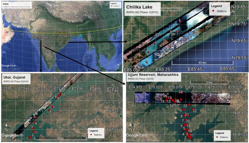
Table 1. Observed ranges of water quality parameters in the three sites.

Site	Sampling period	Chl-a$\mathit{ }(\mathrm{mg}/{\mathrm{m}}^3)$	N
Chilika lake	24–27 December, 2015	6.18–15.55	6
Vallabh Sagar reservoir (Ukai)	27–28 March, 2018	5.01–16.74	10
Ujjani reservoir	3–4 March, 2018	15.76–33.14	22

3.1. Reflectance measurements in Chilika lagoon

The surface downwelling irradiance ($E_d$) and upwelling radiance ($L_u$) measurements in Chilika lake were measured using a Satlantic underwater hyperspectral radiometer (Sahay et al. 2019). The radiometer operates in 256 channels covering the wavelength range of 350–800 nm with 10 nm spectral resolution and sampling rate of 3.3 nm/pixel. The water-leaving radiance is obtained from the upwelling radiance using the following equation (1) $$L_w\left(0^{+},\lambda \right)=L_u\left(0^{-},\lambda \right)\frac{1-\rho \left(\lambda \right)}{{\eta }_w^2\left(\lambda \right)}$$(1) where $L_w\left(0^{+},\lambda \right)$ is the water-leaving radiance just above the water surface; $L_u(0^{-},\lambda )$ is the water-leaving radiance just below the water surface; $\rho (\lambda )$ is the Fresnel reflectance index of water and ${\eta }_w(\lambda )$ is the refractive index of water. The normalized water-leaving radiance, $L_{wn}(\lambda )$ and surface remote-sensing reflectance are calculated using Eqs. (2)(2) $$L_{wn}\left(\lambda \right)=L_w\left(\lambda \right)\mathrm{ }\frac{F_o\left(\lambda \right)}{E_d(0^{+},\lambda )}$$(2) and (3)(3) $$R_{rs}\left(0^{+},\lambda \right)=\frac{L_w\left(0^{+},\lambda \right)}{E_d(0^{+},\lambda )}$$(3) (Mueller et al. 2004) (2) $$L_{wn}\left(\lambda \right)=L_w\left(\lambda \right)\mathrm{ }\frac{F_o\left(\lambda \right)}{E_d(0^{+},\lambda )}$$(2) (3) $$R_{rs}\left(0^{+},\lambda \right)=\frac{L_w\left(0^{+},\lambda \right)}{E_d(0^{+},\lambda )}$$(3) (4) $$E_d\left(0^{+},\lambda \right)=E_d\left(0^{-},\lambda \right)/(1-\alpha )$$(4) where $F_0(\lambda )$ is the extra-terrestrial solar irradiance. $E_d\left(0^{+},\lambda \right)$ denotes downwelling spectral irradiance measured just above the water surface; The Fresnel reflectance value ($\alpha$) for irradiance from the sun and sky is 0.043.

3.2. Reflectance measurements in Vallabhsagar and Ujjani reservoirs

Measurements of water-leaving radiance $(L_u(\lambda )),$ downward radiance of skylight $(L_{\mathit{sky}}(\lambda ))$ and the downward irradiance $(E_d(\lambda )),$ were taken following the method specified in Mueller et al. (2003). The measurements were made above-water using 1) FieldSpec Handheld Spectroradiometer (Analytical Spectral Devices, Boulder, CO) in the range of 325 to 1075 nm at 1 nm intervals and 2) GER-1500 Spectroradiometer (Spectra Vista Corporation, USA). The above-water $R_{rs}(\lambda )$ was calculated using Eq. (5)(5) $$R_{rs}\left(\lambda \right)=\left(\frac{L_u\left(\lambda \right)-r{L}_{\mathit{sky}}\left(\lambda \right)}{E_d\left(\lambda \right)}\right)\times Cal\left(\lambda \right)\times 100$$(5) (Mobley 1999) (5) $$R_{rs}\left(\lambda \right)=\left(\frac{L_u\left(\lambda \right)-r{L}_{\mathit{sky}}\left(\lambda \right)}{E_d\left(\lambda \right)}\right)\times Cal\left(\lambda \right)\times 100$$(5) where $r$ is skylight reflectance determined based on wind speed. A grey Spectralon standard reflectance panel (Labsphere, North Sutton, NH) is used as a reference, and the spectral reflectance calibration factor is $\mathit{Cal}(\lambda ).$ As the inland waters are turbid, the assumption of zero reflectance at 765 or higher wavelengths does not hold and offset correction is not applied (Mueller et al. 2004). 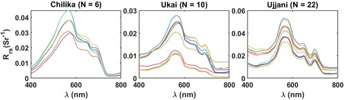The $R_{rs}(\lambda )$ collected from the three water bodies are presented in Figure 2.

Figure 2. In situ above-water measured reflectance measurements from Chilika Lake, Ukai Reservoir and Ujjani Reservoir.

Water samples collected at 38 stations for Chl-a were filtered on the day of collection through Whatman Polycarbonate filters (47 mm diameter, $0.22 \mathrm{\mu }\mathrm{m}$) at low vacuum pressure. The filtrate was extracted using acetone (90%) at 4 °C for 24 h in the dark, and absorbance measurements of the extracted filtrate were taken using a Hitachi Spectrophotometer. Using the absorbance measurements at four wavelengths 630, 647, 663 and 750 nm, the concentration of Chl-a is calculated based on the standard equations (Jeffrey and Humphrey 1975). Similar to Chl-a, water samples for CDOM at 38 stations were collected and filtered through 0.2 $\mathrm{\mu }\mathrm{m}$ pore size Nucleopore membrane filters, and samples were stored in the refrigerator until analysis. The CDOM absorption in the 400–800 nm range was determined by measuring the absorption from the filtered sample placed in a one cm clean quartz cuvette in Hitachi Spectrophotometer. The measured absorbances were converted into absorption coefficients using (6) $$a_g\left(\lambda \right)=2.303\times A\left(\lambda \right)/l$$(6) where $a_g(\lambda )$ and $A(\lambda )$ are the measured absorption coefficients [m⁻¹] and absorbance, respectively, and $l$ is the path length in m.

3.3. AVIRIS-NG reflectance products and Sentinel-3 OLCI imagery

NASA’s AVIRIS-NG sensor acquired hyperspectral imagery over the three sites as a part of the NASA-ISRO joint mission. AVIRIS-NG sensor was mounted on a ISRO B200 aircraft with nadir viewport, flying at an altitude of 4 km (Hamlin et al. 2011, Bhattacharya et al. 2019). The sensor has a 34^° Field of View (FOV) and 1 mrad Instantaneous FOV. The flight altitude ranges between 4 and 8 km, with a swath of 4 to 6 km, and ground sampling distance of 4 to 8 m (Ratheesh et al. 2019). The hyperspectral imagery has a high signal-to-noise ratio of >2000 @600 nm and >1000 @2200 nm in the solar reflected spectral range. The sampling rate is 5 nm and the wavelength range covered is 380 to 2510 nm (Vane et al. 1993; Green et al. 1998; Bhattacharya et al. 2016). AVIRIS-NG level 2 products are reflectance products obtained after applying Atmospheric REMoval atmospheric correction on the Level 1 radiance data (Bo-Cai et al. 1999). Two Level-2 AVIRIS-NG hyperspectral images (4 m spatial resolution) acquired over Ujjani Reservoir at 8:26 UTC (13:56 IST) and 8:36 UTC (14:06 IST) on 3 March 2018 are obtained from AVIRIS-NG data portal (https://avirisng.jpl.nasa.gov/dataportal/). In addition, one AVIRIS-NG Level 2 reflectance product acquired on 5:51 UTC (11:21 IST), 27 December 2015 over Chilika lake with 8 m spatial resolution is also used. A portion of the two AVIRIS-NG scenes from Ujjani reservoir are affected by haze, and hence a haze correction method specifically developed hyperspectral imagery over inland water bodies (Kolluru et al. 2021) is used to remove the haze effects. The present study uses haze-corrected hyperspectral imagery only for the generation of Chl-a maps in case of Ujjani reservoir. In the case of Chilika lake, no haze was present in the scenes under consideration, hence no haze correction was applied.

Level 2 OLCI surface reflectance products (Doerffer 2010) covering Chilika lake (2019 & 2020) corrected for atmospheric effects were obtained from https://coda.eumetsat.int/. L2 OLCI product contains 15 spectral bands in the range of 420–1000 nm. The spectral channel around 673 nm is generally used to improve the accuracy of Chl-a estimations (Moses et al. 2019). The spatial resolution of OLCI data is about 300 m. OLCI data acquired over Chilika lake spanning between January 2019 and November 2020 are used for the study. The spectral channels centered around 673, 709 and 753 nm wavelengths only are used for implementation of the tuned red-NIR algorithms.

3.4. Blue-green and red-NIR algorithms

The blue-green algorithms OC3E, OC4E and OC4Me (where OC stands for Ocean Color), were selected to retrieve Chl-a. These blue-green algorithms perform well in clear waters but exhibited poor performance in turbid waters. These algorithms employ a polynomial type of relation between $R_{rs}$ in the blue-green region (visible spectrum) at 3 or 4 wavelengths and Chl-a. The OCx is a fourth-order polynomial relationship of the following form and relates Chl-a concentration and $R_{rs}$ (7) $${\log }_{10}(\mathit{Chl}-a)=a0+\sum _{i=1}^4{a}_i\mathrm{ }{\left({\log }_{10}\left(\frac{R_{rs}\left({\lambda }_{\mathit{blue}}\right)}{R_{rs}\left({\lambda }_{\mathit{green}}\right)}\right)\right)}^i$$(7) where the numerator, R_rs (λ_blue) is the greatest of several input R_rs values in the blue region, and a0-a4 are sensor-specific coefficients (https://oceancolor.gsfc.nasa.gov). Table 2 lists different algorithms used to retrieve Chl-a from the Medium Resolution Imaging Spectrometer (MERIS). The coefficients given are modified based on field-measured concentrations of Chl-a worldwide cruises (O’Reilly and Maritorena 2000). OC3E and OC4E algorithms use three and four bands in blue-green region of the electromagnetic spectrum and are specifically tuned for MERIS sensor. OC4ME is similar to OC4E, except for the coefficients are obtained from a study by Morel and Antoine (2011).

Table 2. Ocean color empirical algorithms are used to estimate Chlorophyll-a in Case I waters (O’Reilly and Maritorena 2000). The OC algorithms considered here are tuned for the MERIS sensor. OC4Me is similar to OC4E but from Morel and Antoine (2011). The green wavelength for all three algorithms is 560 nm.

Algo-rithm	Blue wavelength in nm	a0	a1	a2	a3	a4
OC3E	Max (443,490)	0.2521	−2.2146	1.5193	−0.7702	−0.4921
OC4E	Max (443, 490, 510)	0.3255	−2.7677	2.4409	−1.1288	−0.4990
OC4Me	Max (443, 490, 510)	0.4502748	−3.259491	3.522731	−3.359422	0.949586

Eleven red-NIR algorithms (Table 3) from the literature are selected to estimate Chl-a from turbid waters and are used for comparison with the blue-green algorithms. The existing red-NIR algorithms use multiple wavelengths in the red-NIR region. The 3-band index-based algorithms relate pigment concentration to $R_{rs}\left({\lambda }_3\right)\times \left(\left(\frac{1}{R_{rs}\left({\lambda }_1\right)}\right)-\left(\frac{1}{{R_{rs}(\lambda }_2)}\right)\right)$ (Dall’Olmo and Gitelson 2005). The position of the first wavelength is chosen such that $R_{rs}({\lambda }_1)$ is maximally sensitive to pigment concentration and minimally sensitive to absorption and scattering by other particles and pigments. The position of the second wavelength is chosen such that it is minimally sensitive to pigment concentration of interest and has similar sensitivity as $R_{rs}({\lambda }_1)$ to absorption and scattering by particulates. Hence, the concentration of pigment can be related directly to the difference $\left[\left(\frac{1}{R_{rs}\left({\lambda }_1\right)}\right)-\left(\frac{1}{{R_{rs}(\lambda }_2)}\right)\right].$ As this difference is still susceptible to scattering by particulate material, ${\lambda }_3$ is chosen such that $R_{rs}({\lambda }_3)$ is minimally sensitive to absorption by all particulate material and can account for variability in scattering by particulate material. Two types of 2-band index-based algorithms exist. The first type relates $R_{rs}({\lambda }_3)/R_{rs}({\lambda }_1)$ to Chl-a concentration, with, ${\lambda }_3$ in NIR region beyond 730 nm and ${\lambda }_1$ in red region. This type of model is more suitable to waters with insignificant contributions by CDOM and NAP (Dall’Olmo and Gitelson 2005). The second type of algorithm relates $R_{rs}({\lambda }_1)/R_{rs}({\lambda }_2)$ to Chl-a concentration, with ${\lambda }_2$ in reflectance peak region of 700–710 nm and ${\lambda }_1$ in red region (Gitelson 1992). To reduce the effects of absorption and backscattering by inorganic material at ${\lambda }_3,$ the term $R_{rs}({\lambda }_3)$ in 3-band index-based algorithm is replaced by Le et al. (2009) with the difference $\left[\left(\frac{1}{R_{rs}({\lambda }_4)}\right)-\left(\frac{1}{R_{rs}({\lambda }_3)}\right)\right],$ ${\lambda }_4$= 740 nm and ${\lambda }_3$ = 704 nm.

Table 3. Existing Red-NIR algorithms used in Chlorophyll-a concentration estimation in turbid productive waters.

Type	Name	Model parameterization	$\mathit{\lambda }(\mathbf{nm})$	Reference
2-band index-based algorithms $\mathrm{RN}2\mathrm{ }=R_{rs}({\lambda }_1)/R_{rs}({\lambda }_2)$	Gurlin2B	25.25 × (RN2^2) + 14.85 × (RN2) − 15.18	${\lambda }_1$ = 709, ${\lambda }_2$ = 665	(Gurlin et al. 2011)
	Gilerson2B	((35.75 × RN2) − 19.30)^1.124	${\lambda }_1$ = 709, ${\lambda }_2$ = 665	(Gilerson et al. 2010)
	Moses2B	61.324 × RN2 − 37.94	${\lambda }_1$ = 709, ${\lambda }_2$ = 665	(Moses et al. 2009)
	Gitelson2B	72.66 × RN2 − 46.535	${\lambda }_1$ = 709, ${\lambda }_2$ = 665	(Gitelson et al. 2011)
	NDCI	$RN= \frac{R_{rs}\left({\lambda }_2\right)-R_{rs}\left({\lambda }_1\right)}{R_{rs}\left({\lambda }_2\right)+R_{rs}\left({\lambda }_1\right)}$ NDCI = 14.039 + (86.115 × RN) + (194.325 × RN^2)	${\lambda }_1$ = 708, ${\lambda }_2$ = 665	(Mishra et al. 2014; Mishra and Mishra 2012)
3-band index-based algorithms RN3 = $R_{rs}\left({\lambda }_3\right) \times \left(\frac{1}{R_{rs}\left({\lambda }_1\right)}-\frac{1}{R_{rs}\left({\lambda }_2\right)}\right)$	Gurlin3B	315.50 × (RN3^2) + 215.95 × RN3 + 25.66	${\lambda }_1$ = 665, ${\lambda }_2$ = 709, ${\lambda }_3$ = 754	(Gurlin et al. 2011)
	Gilerson3B	((113.36 × RN3) + 16.45)^1.124	${\lambda }_1$ = 665, ${\lambda }_2$ = 709, ${\lambda }_3$ = 754	(Gilerson et al. 2010)
	Moses3B	232.29 × RN3 + 23.174	${\lambda }_1$ = 665, ${\lambda }_2$ = 709, ${\lambda }_3$ = 754	(Moses et al. 2009)
	Gitelson3B	243.862 × RN3 + 27.219	${\lambda }_1$ = 665, ${\lambda }_2$ = 709, ${\lambda }_3$ = 754	(Gitelson et al. 2011)
Four-band index-based algorithms	L4B	(20.55 × RN4) + 5.23; $\mathrm{RN}4\mathrm{ }=(R_{rs}{\left({\lambda }_1\right)}^{-1}- R_{rs}{\left({\lambda }_2\right)}^{-1})/(R_{rs}{\left({\lambda }_4\right)}^{-1}- R_{rs}{\left({\lambda }_3\right)}^{-1})$	${\lambda }_1$ = 665, ${\lambda }_2$ = 681, ${\lambda }_3$ = 709, ${\lambda }_4$ = 681.	(Le et al. 2013)
	SCI	$H_{\mathrm{chl}}=\left[R_{rs}\left({\lambda }_4\right)+\frac{{\lambda }_4-{\lambda }_3}{{\lambda }_4-{\lambda }_2}\left(R_{rs}\left({\lambda }_2\right)- R_{rs}\left({\lambda }_4\right)\right)\right]-R_{rs}\left({\lambda }_3\right)$; $H_{\mathrm{\Delta }} = R \left[R_{rs}\left({\lambda }_4\right)+\frac{{\lambda }_4-{\lambda }_3}{{\lambda }_4-{\lambda }_2}\left(R_{rs}\left({\lambda }_2\right)- R_{rs}\left({\lambda }_4\right)\right)\right];$ $\mathit{SCI}=H_{\mathit{chl}}-H_{\mathrm{\Delta }}$ $\mathit{Chl}-a =0.057\mathrm{ }\times \mathrm{ }\mathrm{SCI}-0.6327$	${\lambda }_1$ = 560, ${\lambda }_2$ = 620, ${\lambda }_3$ = 665, ${\lambda }_4$ = 681	(Shen et al. 2010)

Shen et al. (2010) proposed SCI to minimize the impact of high turbidity on the fluorescence line height algorithm in the estimation of Chl-a. NDCI is an index developed with inspiration from the widely used Normalized Difference Vegetation Index (NDVI) for land-based applications (Mishra and Mishra 2012). NDCI was proposed to eliminate uncertainties pertaining to the estimation of $R_{rs},$ seasonal change in solar azimuth differences and atmospheric contribution at the two wavelengths.

4. Results

Firstly, the performance of the selected Chl-a estimation algorithms is assessed. Next, the optimal wavelengths in red-NIR algorithms that result in the least errors to estimate Chl-a concentration are found by the proximal sensing method. Then, the performance of the tuned red-NIR algorithms and existing algorithms is evaluated on a validation dataset. The best performing red-NIR algorithm is applied to AVIRIS-NG and OLCI images to study the spatial and temporal variability of Chl-a concentration.

4.1. Performance of the selected algorithms

The performance comparison of all fourteen algorithms over the complete dataset collected from the three water (N = 38) bodies is presented in Table 4. All 2-band and 3-band index-based algorithms resulted in lower RMSE and MAE values with ranges 4.84–6.17 $\mathrm{mg}/{\mathrm{m}}^3$ and 3.83–4.65 $\mathrm{mg}/{\mathrm{m}}^3.$ The NDCI and four-band index-based algorithms resulted in higher errors than the 2-band and 3-band index-based algorithms. The three blue-green algorithms also resulted in higher RMSE and MAE values with lower $R^2$ values. Although the red-NIR algorithms resulted in lower RMSE and MAE values, higher MAPE values were observed (>50%). These results indicate that red-NIR algorithms can derive Chl-a; however, further tuning with in situ measured $R_{rs}(\lambda )$ and Chl-a is necessary to reduce the errors.

Table 4. Performance of various existing red-NIR and blue-green algorithms for the complete dataset.

	Model	RMSE ($\mathrm{mg}/{\mathrm{m}}^3$)	MAPE (%)	Bias ($\mathrm{mg}/{\mathrm{m}}^3$)	MAE ($\mathrm{mg}/{\mathrm{m}}^3$ )	${\mathit{R}}^2$	n
Blue-Green type	OC3E	12.59	86.17	4.22	10.56	0.18	38
	OC4E	12.06	81.65	4.28	10.04	0.24	38
	OC4Me	41.22	41.07	−17.68	21.32	0.19	38
Red-NIR type	Gurlin2B	5.03	73.78	2.74	4.05	0.87	38
	Gurlin3B	5.56	77.38	1.50	4.65	0.79	38
	Gilerson2B	5.55	104.68	3.76	4.59	0.87	38
	Gilerson3B	5.83	58.36	2.97	4.89	0.79	37
	L4B	40.56	462.56	−14.57	21.66	0.24	38
	NDCI	9.73	92.84	8.63	8.63	0.89	38
	SCI	16.81	506.01	15.10	15.10	0.41	38
	Moses2B	5.70	172.04	3.34	4.44	0.86	37
	Moses3B	6.03	666.68	2.33	4.82	0.77	33
	Gitelson2B	4.84	705.95	2.18	3.83	0.88	32
	Gitelson3B	6.17	137.42	1.14	4.89	0.76	34

4.2. Tuning red-NIR algorithms for finding optimal wavelengths

4.2.1. Calibration of 2-band and 3-band red-NIR algorithms

The bio-optical variability observed in natural water bodies affects the optimal spectral bands chosen in the 2-band and 3-band index-based algorithms. To find the optimal wavelengths of ${\lambda }_1, { \lambda }_2$ and ${\lambda }_3$ for the present dataset, an optimization technique is employed as suggested in Dall’Olmo and Gitelson (2005).

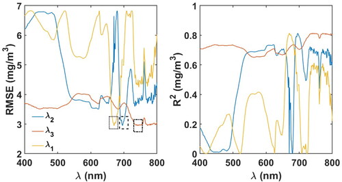
The calibration dataset consists of 20 samples covering all three water bodies with various optical properties. The two wavelengths ${\lambda }_1$ and ${\lambda }_3$ were set to 670 nm and 740 nm to find the optimal position of ${\lambda }_2.$ These wavelengths were chosen as 670 nm falls in the range of maximum Chl-a red absorption, and at 740 nm, the variation in particulate backscattering controls the variations in reflectance. The model $\left[R_{rs}^{-1}\left(670\right)-R_{rs}^{-1}\left({\lambda }_2\right)\right]\times R_{rs}(740)$ was regressed against Chl-a in the range of 600–750 nm. The RMSE values of Chl-a estimation were lower for ${\lambda }_2$ in the range of 680–715 nm with a minimum at 696 nm (Figure 3). In the second iteration, the optimal wavelength range for ${\lambda }_3$ was found by fixing ${\lambda }_2$ to 696 nm, and regressing the model $\left[R_{rs}^{-1}\left(670\right)-R_{rs}^{-1}\left(696\right)\right]\times R_{rs}({\lambda }_3)$ vs. Chl-a. 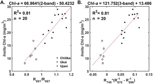The RMSE was minimal in the range of 735–755 nm for ${\lambda }_3.$ In the third iteration, the optimal wavelength range for ${\lambda }_1$ was found by fixing ${\lambda }_2$ and ${\lambda }_3$ to 696 nm and 740 nm, respectively and by regressing $\left[R_{rs}^{-1}\left({\lambda }_1\right)-R_{rs}^{-1}\left(696\right)\right]\times R_{rs}(740)$ vs. Chl-a. The RMSE values were minimal in 665–685 nm, with a minimum value at 670 nm. The 3-band tuned algorithm has the form (8) $$\mathrm{Chl}–\mathrm{a}\mathrm{ }=121.752\mathrm{ }\times \left(R_{rs}\left(740\right)\times \left(\frac{1}{R_{rs}\left(670\right)}-\frac{1}{R_{rs}\left(696\right)}\right)\right)+13.486$$(8)

Figure 3. RMSE and R² values obtained in tuning the 3-band model. THE least RMSE values were obtained at 670, 696 and 740 nm for ${\lambda }_1, {\lambda }_2$ and ${\lambda }_3,$ respectively. The regions of least RMSE’s for ${\lambda }_1, {\lambda }_2$ and ${\lambda }_3$ are represented with a black-dotted rectangle, black-dashed rectangle and black dot-dashed rectangles, respectively.

The 2-band model, $R_{rs}({\lambda }_1)/R_{rs}({\lambda }_2),$ was calibrated by fixing ${\lambda }_1$ at each wavelength in the entire range of 400–800 nm and varying ${\lambda }_2$ and regressing the ratio against Chl-a concentration (Figure 4). The 2-band ratio of $R_{rs}\left(691\right)/R_{rs}(667)$ resulted in the least RMSE and highest $R^2$ with the form (Figure 5A). (9) $$\mathrm{Chl}–\mathrm{a}\mathrm{ }=66.9641\mathrm{ }\times \mathrm{ }\left(\frac{R_{rs}\left(691\right)}{R_{rs}\left(667\right)}\right)+50.432$$(9)

Figure 4. RMSE and R² values obtained in tuning the 2-band Red-NIR model. The Least RMSE and highest $R^2$ values were obtained for ${\lambda }_1$ = 667 nm and ${\lambda }_2=$ 691 nm, respectively.

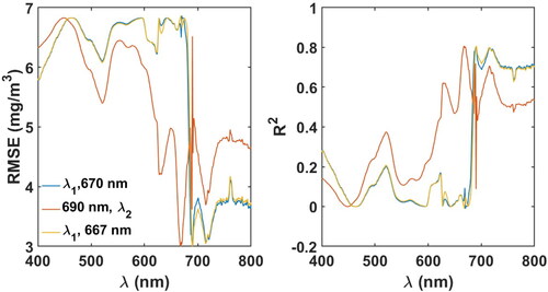
Figure 5. Calibration results of tuned A). 2-band and B). 3-band red-NIR algorithms.

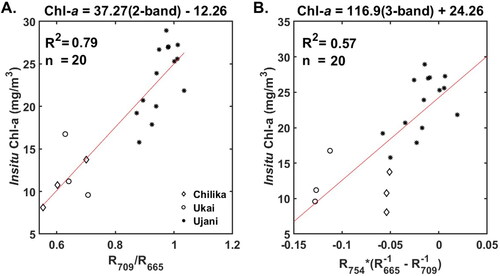
To facilitate application of the tuned red-NIR algorithms to the existing Sentinel-3 OLCI sensor and past MERIS sensor data, the 3-band algorithm was re-calibrated with the wavelengths ${\lambda }_1$ = 665 nm, ${\lambda }_2$ = 709 nm and ${\lambda }_3$ = 754 nm (Figure 6B). Similarly, the 2-band algorithm was re-calibrated with 709 nm and 665 nm (Figure 6A). The 3- and 2-band OLCI wavelength tuned algorithms have the form (10) $$\mathrm{Chl}–\mathrm{a}\mathrm{ }=116.9\mathrm{ }\times \left(R_{rs}\left(754\right)\times \left(\frac{1}{R_{rs}\left(665\right)}-\frac{1}{R_{rs}\left(709\right)}\right)\right)+24.26$$(10) (11) $$\mathrm{Chl}–\mathrm{a}\mathrm{ }=37.27\mathrm{ }\times \mathrm{ }\left(\frac{R_{rs}\left(709\right)}{R_{rs}\left(665\right)}\right)-12.26$$(11)

Figure 6. Calibration of A). 2-band and B). 3-band red-NIR algorithms with OLCI wavelengths.

4.2.2. Evaluating accuracy of the tuned red-NIR algorithms

This section presents the performance evaluation of 3-band and 2-band tuned algorithms and 3- and 2-band with OLCI wavelengths. A validation dataset consists of 18 samples covering all three water bodies is used to compare estimated and measured Chl-a.

The comparison of the measured Chl-a and predicted Chl-a estimates by the 3-band tuned and 3-band OLCI wavelengths algorithms are presented are Figures 7 and 8 and Table 5. The tuned 3-band algorithm resulted in the lowest MAPE value of 22.56% and RMSE of 4.24 $\mathrm{mg}/{\mathrm{m}}^3.$ The $R^2$ value of 0.90 indicates a strong correlation between measured and the 3-band tuned algorithm predicted Chl-a values. The tuned 2-band algorithm resulted in RMSE and MAPE values of 5.35 $\mathrm{mg}/{\mathrm{m}}^3$ and 29.96%, respectively. The 3-band algorithm with OLCI wavelengths resulted in Chl-a estimates with RMSE and MAPE values of 5.62 $\mathrm{mg}/{\mathrm{m}}^3$ and 27.67%. The $R^2$ (0.80) and bias (−0.49) values obtained for OLCI specific 3-band algorithm indicate higher error than the tuned 3-band algorithm. In the case of OLCI specific 2-band algorithm, the RMSE and MAPE values are 5.18 $\mathrm{mg}/{\mathrm{m}}^3$ and 28.83%, respectively. The RMSE and MAE values of all the four algorithms lie in the same range; however, the 3-band tuned algorithm resulted in the lowest MAPE among the four algorithms.

Figure 7. Validation of the A). 2-band tuned and B). 3-band tuned red-NIR algorithms.

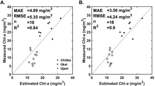
Figure 8. Validation of the A). 2-band and B). 3-band red-NIR algorithms tuned with OLCI specific wavelengths.

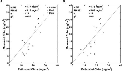
Table 5. Performance of various red-NIR and blue-green algorithms for validation dataset.

	Model	RMSE ($\mathrm{mg}/{\mathrm{m}}^3$ )	MAPE (%)	Bias ($\mathrm{mg}/{\mathrm{m}}^3$ )	MAE ($\mathrm{mg}/{\mathrm{m}}^3$ )	${\mathit{R}}^2$	n
Existing blue-green	OC3E	11.71	104.03	7.73	9.69	0.26	18
	OC4E	11.18	95.52	7.62	9.08	0.45	18
	OC4Me	9.80	38.99	−2.24	7.60	0.44	18
Existing red-NIR	Gurlin2B	5.10	48.48	2.57	4.16	0.88	18
	Gurlin3B	6.12	114.68	1.72	5.31	0.80	18
	Gilerson2B	5.64	57.80	3.53	4.66	0.88	18
	Gilerson3B	6.19	52.17	2.95	5.27	0.81	17
	L4B	47.15	600.3	−18	25.2		18
	NDCI	9.76	88.30	8.11	8.11	0.89	18
	SCI	16.21	424.14	13.68	13.68	0.34	18
	Moses2B	5.73	119.34	3.50	4.55	0.88	18
	Moses3B	6.50	50.22	2.81	5.82	0.81	15
	Gitelson2B	5.09	79.04	2.63	4.11	0.89	15
	Gitelson3B	6.78	128.77	1.99	5.75	0.79	16
This study	Tuned_2band	5.35	29.96	−0.71	4.89	0.84	18
	Tuned_3band	4.24	22.56	−0.24	3.56	0.90	18
	OLCI_2band	5.18	28.83	−1.08	4.77	0.87	18
	OCLI_3band	5.62	27.67	−0.49	4.72	0.80	18

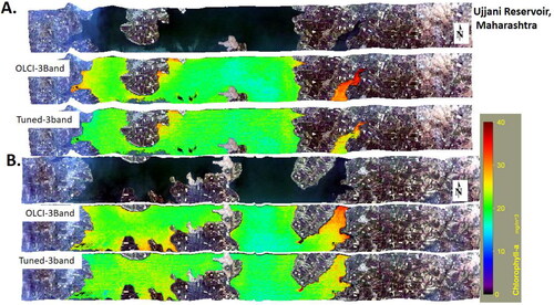
Finally, the tuned 2-band and 3-band, OLCI specific 2-band, and 3-band red-NIR algorithms are applied to AVIRIS-NG imagery. Two strips (Figure 9A, B) of AVIRIS-NG imagery acquired over the Ujjani reservoir are used. The estimated Chl-a concentrations from the AVIRIS-NG imagery lie in the range of 18–30 mg/m³ as observed in the in situ measurements from the Ujjani reservoir (Table 1).

Figure 9. Application of tuned 3-band and OLCI specific 3-band red-NIR algorithms to estimate Chlorophyll-a from two AVIRIS-NG imagery acquired over Ujjani Reservoir, Maharashtra.

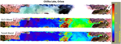
Similarly, the tuned and OLCI specific Chl-a algorithms are applied to one strip of AVIRIS-NG imagery acquired over Chilika lake (Figure 10). The southern sector of Chilika lake is relatively clear, as indicated by lower Chl-a concentration as compared to the northern sector, which is highly influenced by terrestrial runoff (Sahu et al. 2016). These results suggest that the tuned Chl-a algorithms can estimate varying levels of Chl-a and in water bodies with varying levels of optical complexity.

Figure 10. Application of tuned 3-band and OLCI specific 3-band red-NIR algorithms to estimate Chlorophyll-a from AVIRIS-NG imagery acquired over Chilika lake, Orissa.

Finally, to check the OLCI sensor tuned 3-band red-NIR algorithm’s applicability, OLCI/Sentinel-3 scenes acquired over Chilika lake from 2019 and 2020 are used. The $R_{rs}$ at 675, 709 and 754 is used as input to Eq. (10)(10) $$\mathrm{Chl}–\mathrm{a}\mathrm{ }=116.9\mathrm{ }\times \left(R_{rs}\left(754\right)\times \left(\frac{1}{R_{rs}\left(665\right)}-\frac{1}{R_{rs}\left(709\right)}\right)\right)+24.26$$(10) to estimate Chl-a concentration. The tuned algorithm is able to differentiate varying Chl-a concentration levels (Figures 11 and 12) in Chilika lake in different months.

Figure 11. Application of OLCI wavelengths tuned 3-band red-NIR algorithm to 10 OLCI/Sentinel-3 scenes in 2019 to estimate Chlorophyll-a concentration.

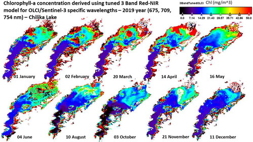
Figure 12. Application of OLCI wavelengths tuned 3-band red-NIR algorithm to 10 OLCI/Sentinel-3 scenes in 2020 to estimate Chlorophyll-a concentration.

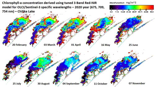
As observed in the AVIRIS-NG scene (Figure 10), the Lake’s Northern sector is affected by terrestrial runoff and river discharge. Also, the runoff and river discharge vary in different months, as observed by varying levels of Chl-a over the ten scenes in the Northern sector. The observed range of in-situ Chl-a concentration values in Chilika lake is 6–15 mg/m³. The field work for collection of these water samples was conducted in December 2018 in middle and southern sectors of the Chilika lake. The Chl-a concentrations for December 2019 and November 2020 (Figures 11 and 12) indicate that in Southern-Middle portions of the Chilika lake, the Chl-a concentrations are between 7 and 14 $\mathrm{mg}/{\mathrm{m}}^3,$ thereby matching the observed range of the in-situ Chl-a concentration values. These results indicate that the tuned OLCI specific 3-band red-NIR algorithm can be used for routine monitoring of Chl-a changes in the Chilika lagoon.

Seasonal variations in Chilika lake are studied based on the following grouping: pre-monsoon (March–June), monsoon (July–October) and post-monsoon (November–February). The spatial and seasonal variation in Chl-a concentration patterns observed in Chilika lake during 2019 and 2020 lie in accordance with previous studies. During 2019 and 2020, NS was the most productive sector of the lagoon in the pre-monsoon season, as observed in 1998–2001 and 2013–2014 (Nayak et al. 2004; Sahoo et al. 2017). The observed Chl-a concentrations levels in NS sector from December 2019 and November 2020 (Figures 11 and 12) are in the range of 20–28 mg/m³, similar concentration levels are reported in Sahoo et al. 2017 (their Fig. 5.c & 5.f) in post-monsoon season. Coincident mixing of sediments and terrestrial runoff during monsoon season reduces light penetration, leading to a relatively lower phytoplankton growth (Mallin et al. 2009; Sahoo et al. 2017).

5. Discussion

Each water-body exhibits different spatial and temporal patterns in optical properties (Moore et al. 2014). Hence, the algorithms developed for a particular water body may not be applied directly to other regions. For the United States inland waters, the suggested optimal spectral bands are 671 nm, 710 nm and 740 nm for 3-band and 665 nm and 725 nm for 2-band algorithms (Gitelson et al. 2007). For the 3-band algorithm, the recommended spectral ranges (Gitelson et al. 2007) for ${\lambda }_1,{\lambda }_2$ and ${\lambda }_3$ with different accuracies are presented in Appendix Table A1. In the present study, the optimal wavelengths for 2-band and 3-band algorithms are (667 nm, 691 nm) and (670 nm, 696 nm and 740 nm) for three water bodies exhibiting different optical properties. These wavelengths lie close to the recommended optimal wavelength ranges. A study by Dall’Olmo and Gitelson (2005) indicated that the maximum RMSE for both 2-band and 3-band algorithms were obtained at ${\lambda }_1$ = 683 nm and a higher RMSE occurs at ${\lambda }_1$ = 683 nm and ${\lambda }_3$ = 750 for 2-band algorithms. In a study by Gitelson et al. (2007), a shift of ${\lambda }_1$ from 667 to 678 nm resulted in an increase in RMSE from 10.7 to 12.7 $\mathrm{mg}/{\mathrm{m}}^3.$ The observed higher RMSE with ${\lambda }_1$ at 683 nm is attributed to variability in Chl-a fluorescence quantum yield (Gitelson et al. 2007). The optimal ${\lambda }_1$ for the 3-band algorithm tuned in the present study is 670 nm that lies close to the recommended range of 671–680 nm. Similarly, the optimal ${\lambda }_2$ = 696 nm and ${\lambda }_3$ = 740 nm obtained in the present study lie in the recommended wavelength ranges of 691–720 nm and 705–769 nm. In particular the optimal wavelengths for the 3-band tuned algorithms in the present study are similar to the wavelengths reported by two other studies (Le et al. 2009, 2013).

We used the validation dataset to evaluate the tuned 2-band and 3-band algorithms and compare their performance with existing red-NIR algorithms. The comparison of the fourteen red-NIR algorithms and four tuned algorithms is presented in Table 5. The 2-band index-based algorithms Gurlin2B, Gilerson2B, Moses2B and Gitelson2B resulted in RMSE values in the range of 5.09–5.64 $\mathrm{mg}/{\mathrm{m}}^3$ and MAPE values in the range of 48–119%. The 3-band index-based algorithms Gurlin3B, Gilerson3B, Moses3B and Gitelson3B also resulted in slightly higher RMSE and MAPE values than the corresponding 2-band index-based algorithms. The blue-green algorithms resulted in RMSE and MAPE values in the range of 9.80–11.71 $\mathrm{mg}/{\mathrm{m}}^3$ and 38–104%, respectively. The four band algorithms also resulted in higher RMSE values in the range 16–47 $\mathrm{mg}/{\mathrm{m}}^3.$ The poor performance of blue-green algorithms resonates with another independent study (Lotliker et al. 2016). The 2-band and 3-band tuned algorithms exhibited lower MAPE values as compared to all existing red-NIR algorithms.

These results indicate that tuning the 3-band and 2-band red-NIR algorithms is essential for estimating Chl-a concentration in inland turbid productive waters. In addition, more data from other geographic locations in India can increase the robustness and applicability to other study areas.

6. Summary and conclusions

The present study focuses on the estimation of Chl-a concentration using in situ measured $R_{rs}(\lambda )$ from three water bodies exhibiting different optical properties. An initial evaluation of various existing blue-green and red-NIR algorithms across the three water bodies indicated that red-NIR algorithms resulted in lower RMSE values than blue-green algorithms. However, higher MAPE values were obtained for the 2-band and 3-band type red-NIR algorithms. Hence, tuning of 2-band and 3-band red-NIR algorithms is performed to obtain optimal wavelengths. Lower RMSE and high correlation coefficients were obtained at ${\lambda }_1$ = 667 nm and ${\lambda }_2$ = 691 nm for 2-band type red-NIR algorithm. Similarly, for the 3-band type red-NIR algorithm, the optimal wavelengths resulting in the least RMSE and high $R^2$ are ${\lambda }_1$ = 670 nm, ${\lambda }_2$ = 696 nm and ${\lambda }_3$ = 740 nm. The 3-band tuned algorithm obtained lower RMSE and MAPE values compared to the 2-band tuned algorithm. The tuned 2-band and 3-band red-NIR algorithms also resulted in lower RMSE and MAPE values for the validation dataset compared to fourteen existing blue-green and red-NIR algorithms. To facilitate regular monitoring using the existing multispectral OLCI sensor, the 2-band algorithm is re-calibrated with 665 nm and 709 nm. Similarly, the 3-band algorithm is re-calibrated with 665 nm, 709 nm and 754 nm wavelengths in the OLCI sensor. The tuned 2-band and 3-band red-NIR algorithms were applied to AVIRIS imagery obtained over the three water bodies. Both tuned and OLCI wavelength-specific 2-band and 3-band algorithms showed variation in Chl-a concentrations in all the water bodies. The results presented here indicate the potential of 2-band and 3-band red-NIR algorithms in the estimation of Chl-a concentration in turbid productive waters using in situ measured $R_{rs}(\lambda ).$

Disclosure statement

No potential conflict of interest was reported by the authors.

Data availability statement

AVIRIS-NG data used for the study is publicly accessible at https://avirisng.jpl.nasa.gov/dataportal/.

Additional information

Funding

This work was funded by Indian Space Research Organisation. The field work is carried out in the three study areas as a part of NASA AVIRIS-NG and ISRO’s Joint program held from 2015 to 2018. Funding to collect data in Ujani Reservoir study area is through the grant RD/0118-ISROC00-004 awarded to Prof. Shirishkumar S. Gedam (Principal Investigator) from CSRE, IIT Bombay by ISRO/SAC Ahmedabad.

Appendix

Table A1. Optimal spectral bands for the 3-band algorithms in different study areas.

Region	${\mathit{\lambda }}_1$	${\mathit{\lambda }}_2$	${\mathit{\lambda }}_3$	RMSE $(\mathrm{mg}/{\mathrm{m}}^3)$	Reference
Chesapeake Bay	674–676	691–698	723–739	<7.9	(Gitelson et al. 2007)
	672–678	689–707	712–762	<8.5
	671–680	688–720	705–780	<9
Kinneret Lake	665	708	753	2.6	(Yacobi et al. 2011)
Tampa Bay	670	695	730	30% (relative error)	(Le et al. 2013)
Fremont State Lake	666	704	723	5.5	(Moses et al. 2012)
Fremont State Lake	670	710	750	1.7	(Gitelson et al. 2009)
Fremont State Lake	666	712	724	2.1	(Gurlin et al. 2011)
NWAC-S	650	710	740	31.9	(Zimba and Gitelson, 2006)
Azov Sea	684	700	720	5	(Gitelson et al. 2011)
University of Florida	680	700	769	13.2	(Abd-Elrahman et al. 2011)
Taihu	660	692	740	5.4	(Le et al. 2009)

References

- Abd-Elrahman A, Croxton M, Pande-Chettri R, Toor GS, Smith S, Hill J. 2011. In situ estimation of water quality parameters in freshwater aquaculture ponds using hyperspectral imaging system. ISPRS J Photogramm Remote Sens. 66:463–472.
- Barik SK, Muduli PR, Mohanty B, Rath P, Samanta S. 2018. Spatial distribution and potential biological risk of some metals in relation to granulometric content in core sediments from Chilika Lake, India. Environ Sci Pollut Res Int. 25(1):572–587.
- Bhattacharya BK, Green RO, Rao S, Saxena M, Sharma S, Ajay Kumar K, Srinivasulu P, Sharma S, Dhar D, Bandyopadhyay S, et al. 2019. An overview of AVIRIS-NG airborne hyperspectral science campaign over India. Curr Sci. 116:1082–1088.
- Bhattacharya BK, Saxena M, Green RO, Rao S, Srinivasulu G, Sharma S, Dhar D, Misra A. 2016. Overview of first phase of AVIRIS-NG airborne hyperspectral science campaign over India. Curr Sci. 116:1082–1088.
- Bo-Cai G, Kathleen BH, Alexander FHG. 1999. ATmosphere REMoval Program (ATREM) User’s Guide, Version 3.1. Center for the Study of Earth from Space (CSES). Boulder (CO): Cooperative Institute for Research in Environmental Sciences (CIRES), Univ. of Colorado.
- Brewin RJW, Raitsos DE, Pradhan Y, Hoteit I. 2013. Comparison of chlorophyll in the Red Sea derived from MODIS-Aqua and in vivo fluorescence. Remote Sens Environ. 136:218–224.
- Brezonik P, Menken KD, Bauer M. 2005. Landsat-based remote sensing of lake water quality characteristics, including chlorophyll and colored dissolved organic matter (CDOM). Lake Reserv Manag. 21:373–382.
- Bricaud A, Babin M, Morel A, Claustre H. 1995. Variability in the chlorophyll-specific absorption coefficients of natural phytoplankton: analysis and parameterization phytoplankton. J Geophys Res. 100:13321–13332.
- Bricaud A, Morel A, Babin M, Allali K, Claustre H. 1998. Variations of light absorption by suspended particles with chlorophyll a concentration in oceanic (case 1) waters: analysis and implications for bio-optical models. J Geophys Res. 103:31033–31044.
- Carlson R. 2007. Estimating Trophic State. Lakeline. 27:25–28.
- Chander S, Gujrati A, Abdul Hakeem K, Garg V, Issac AM, Dhote PR, Kumar V, Sahay A. 2019. Water quality assessment of River Ganga and Chilika lagoon using AVIRIS-NG hyperspectral data. Curr Sci. 116:1172–1181.
- Ciotti M, Lewis MR, Cullen JJ. 2002. Assessment of the relationships between dominant cell size in natural phytoplankton communities and the spectral shape of the absorption coefficient. Limnol. Oceanogr. 47:404–417.
- D’Alimonte D, Zibordi G, Berthon JF, Canuti E, Kajiyama T. 2012. Performance and applicability of bio-optical algorithms in different European seas. Remote Sens Environ. 124:402–412.
- Dall’Olmo G, Gitelson A, Rundquist DC. 2003. Towards a unified approach for remote estimation of chlorophyll-a in both terrestrial vegetation and turbid productive waters. Geophys Res Lett. 30:8–11.
- Dall’Olmo G, Gitelson AA. 2005. Effect of bio-optical parameter variability on the remote estimation of chlorophyll-a concentration in turbid productive waters: experimental results. Appl Opt. 44:3342.
- Doerffer R. 2010. OLCI Level 2 Algorithm Theoretical Basis Document: Ocean Colour Turbid Water, Sentinel-3 L2 Products and Algorithm Definition.
- Fuller I. 2009. Large rivers: geomorphology and management, edited by A. Gupta. 2007. John Wiley & Sons Ltd: Chichester, 712 pages. ISBN: 9780470849873. River Res Appl.; p. 340–341.
- Giardino C, Brando VE, Dekker AG, Strömbeck N, Candiani G. 2007. Assessment of water quality in Lake Garda (Italy) using Hyperion. Remote Sens Environ. 109:183–195.
- Gilerson AA, Gitelson AA, Zhou J, Gurlin D, Moses W, Ioannou I, Ahmed SA. 2010. Algorithms for remote estimation of chlorophyll-a in coastal and inland waters using red and near infrared bands. Opt Express. 18(23):24109–24125.
- Gitelson A. 1992. The peak near 700 nm on radiance spectra of algae and water: relationships of its magnitude and position with chlorophyll concentration. Int J Remote Sens. 13:3367–3373.
- Gitelson AA, Gao B-C, Li R-R, Berdnikov S, Saprygin V. 2011. Estimation of chlorophyll-a concentration in productive turbid waters using a Hyperspectral Imager for the Coastal Ocean—the Azov Sea case study. Environ Res Lett. 6:024023.
- Gitelson AA, Gurlin D, Moses WJ, Barrow T. 2009. A bio-optical algorithm for the remote estimation of the chlorophyll-a concentration in case 2 waters. Environ Res Lett. 4:2–7.
- Gitelson AA, Gurlin D, Moses WJ, Yacobi YZ. 2011. Remote estimation of chlorophyll-a concentration in inland, estuarine, and coastal waters. Adv. Environ. Remote Sens. Sensors, Algorithms, Appl.; Boca Raton, Florida: Taylor and Francis Group, p. 439–468.
- Gitelson AA, Schalles JF, Hladik CM. 2007. Remote chlorophyll-a retrieval in turbid, productive estuaries: Chesapeake Bay case study. Remote Sens Environ. 109:464–472.
- Gons HJ. 1999. Optical teledetection of Chlorophyll a in turbid inland waters. Environ Sci Technol. 33:1127–1132.
- Gordon HR, Brown OB, Evans RH, Brown JW, Smith RC, Baker KS, Clark DK. 1988. A semianalytic radiance model of ocean color. J Geophys Res. 93:10909–10924.
- Green RO, Eastwood ML, Sarture CM, Chrien TG, Aronsson M, Chippendale BJ, Faust JA, Pavri BE, Chovit CJ, Solis M, et al. 1998. Imaging spectroscopy and airborne visible/infrared imaging spectrometer (AVIRIS). Remote Sens Environ. 65:227–248.
- Gupta M. 2013. Chromaticity analysis of the Chilika lagoon for total suspended sediment estimation using RESOURCESAT-1 AWiFS data - a case study. J Great Lakes Res. 39:696–700.
- Gurlin D, Gitelson AA, Moses WJ. 2011. Remote estimation of chl- a concentration in turbid productive waters — return to a simple two-band NIR-red model ? Remote Sens Environ. 115:3479–3490.
- Hamlin L, Green RO, Mouroulis P, Eastwood M, Wilson D, Dudik M, Paine C. 2011. Imaging spectrometer science measurements for terrestrial ecology: AVIRIS and new developments. In: IEEE Aerospace Conference Proceedings, Big Sky, Montana. IEEE, Montana, USA, pp. 1–7.
- Huot Y, Babin M, Bruyant F, Grob C, Twardowski MS, Claustre H, Huot Y, Babin M, Bruyant F, Grob C, et al. 2007. Does chlorophyll a provide the best index of phytoplankton biomass for primary productivity studies ? Biogeosciences Discuss. 4:707–745.
- IOCCG 2006., Remote Sensing of Inherent Optical Properties: fundamentals, Tests of Algorithms, and Applications, Reports of the International Ocean Colour Coordinating Group. Dartmouth, Canada: IOCCG.
- Jeffrey SW, Humphrey GF. 1975. New spectrophotometric equations for determining chlorophylls a, b, c1 and c2 in higher plants, algae and natural phytoplankton. Biochem Physiol Pflanz. 167:191–194.
- Kolluru S, Gedam SS, Inamdar AB. 2021. Haze correction of hyperspectral imagery over inland waters. Geocarto Int. 0:1–18.
- Kumar Jally S, Kumar Mishra A, Balabantaray S. 2020. Estimation of Trophic State Index of Chilika Lake using Landsat-8 OLI and LISS-III satellite data. Geocarto Int. 35:759–780.
- Le C, Hu C, Cannizzaro J, English D, Muller-Karger F, Lee Z. 2013. Evaluation of chlorophyll-a remote sensing algorithms for an optically complex estuary. Remote Sens Environ. 129:75–89.
- Le C, Li Y, Zha Y, Sun D, Huang C, Lu H. 2009. A four-band semi-analytical model for estimating chlorophyll a in highly turbid lakes: the case of Taihu Lake, China. Remote Sens Environ. 113:1175–1182.
- Le C, Li Y, Zha Y, Sun D, Huang C, Zhang H. 2011. Remote estimation of chlorophyll a in optically complex waters based on optical classification. Remote Sens Environ. 115:725–737.
- Lotliker AA, Sahoo S, Baliarsingh SK, Parida C, Sahu KC. 2016. Optical characterization and assessment of ocean colour algorithms in Chilika Lagoon. In: Frouin R, Shenoi SC, Rao KH, editors. SPIE Proceedings. SPIE Asia Pacific Remote Sensing, New Delhi, India; p. 987813.
- Mahapatro D, Barik SK, Rastogi G, Samal RN, Muduli PR, Nair G, Pattanaik AK. 2001. Assessment of physicochemical parameter and it’s influence on macrobenthic community of a brackish water Coastal Ecosystem- The Chilika Lagoon, East Coast of India, International Workshop on Ocean Acidifcation- Consequences for Marine Ecosystems, IISER, Salt Lake City, Kolkata18.
- Mallin MA, Posey MH, Mciver MR, Parsons DC, Ensign H, Alphin TD. 2009. Impacts and from Recovery Multiple Hurricanes Plain River System. Bioscience. 52:999–1010.
- Menon HB, Adhikari A. 2018. Remote sensing of Chlorophyll-A in case II waters: a novel approach with improved accuracy over widely implemented turbid water indices. J Geophys Res Ocean. 123:8138–8158.
- Mishra DR, Schaeffer BA, Keith D. 2014. Performance evaluation of normalized difference chlorophyll index in northern Gulf of Mexico estuaries using the Hyperspectral Imager for the Coastal Ocean. GIScience Remote Sens. 51:175–198.
- Mishra S, Mishra DR. 2012. Normalized difference chlorophyll index: a novel model for remote estimation of chlorophyll-a concentration in turbid productive waters. Remote Sens Environ. 117:394–406.
- Mishra SP, Jena J. 2012. Effects of variable inflow from Northern Major Rivers into the Chilika Lagoon, Odisha, India. Int J Lakes Rivers. 5:123–132.
- Mishra SP, Ojha AC. 2020. Appraising the impact of Naraj barrage on sedimentation of Chilika Lagoon; the soft computing model for prediction. Arch Curr Res Int. 20(6):31–41.
- Mobley CD. 1999. Estimation of the remote-sensing reflectance from above-surface measurements. Appl Opt. 38(36):7442–7455.
- Moore TS, Dowell MD, Bradt S, Ruiz Verdu A. 2014. An optical water type framework for selecting and blending retrievals from bio-optical algorithms in lakes and coastal waters. Remote Sens Environ. 143:97–111.
- Morel A, Antoine D. 2011. ATBD 2.9 - Pigment Index Retrieval in Case 1 Waters.
- Moses WJ, Gitelson AA, Berdnikov S, Povazhnyy V. 2009. Satellite estimation of chlorophyll-a concentration using the red and NIR bands of MERISThe azov sea case study. IEEE Geosci Remote Sens Lett. 6:845–849.
- Moses WJ, Gitelson AA, Perk RL, Gurlin D, Rundquist DC, Leavitt BC, Barrow TM, Brakhage P. 2012. Estimation of chlorophyll-a concentration in turbid productive waters using airborne hyperspectral data. Water Res. 46(4):993–1004.
- Moses WJ, Saprygin V, Gerasyuk V, Povazhnyy V, Berdnikov S, Gitelson AA. 2019. OLCI-based NIR-red models for estimating chlorophyll- a concentration in productive coastal waters—a preliminary evaluation. Environ Res Commun. 1:011002.
- Muduli PR, Kanuri VV, Robin RS, Charan Kumar B, Patra S, Raman AV, Nageswarara Rao G, Subramanian BR. 2012. Spatio-temporal variation of CO2 emission from Chilika Lake, a tropical coastal lagoon, on the east coast of India. Estuar Coast Shelf Sci. 113:305–313.
- Mueller JL, Brown SW, Clark DK, Johnson BC, Yoon H, Lykke KR, Flora SJ, Feinholz M, Souaidia N, Pietras C, et al. 2004. Ocean optics protocols for satellite ocean color sensor validation, Revision 5, Volume VI: Special topics in ocean optics protocols, Part 2. Ocean Color web page VI, 35.
- Mueller JL, Morel AY, Frouin R, Davis C, Arnone R, Carder K, Lee Z, Steward RG, Hooker SB, Mobley CD, et al. 2003. Ocean Optics Protocols For Satellite Ocean Color Sensor Validation, Revision 4, Volume III: Radiometric Measurements and Data Analysis Protocols. Nasa/Tm-2003-21621 III, 78.
- Mukherjee M, Banik SK, Pradhan SK, Sharma AP, Suresh VR, Manna RK, Panda D, Roshith CM, Mandal S. 2015. Diversity and distribution of tintinnids in Chilika Lagoon with description of new records. Indian J Geo-Marine Sci. 62:25–32.
- Nag SK, Saha K, Bandopadhyay S, Ghosh A, Mukherjee M, Raut A, Raman RK, Suresh VR, Mohanty, S, K. 2020. Status of pesticide residues in water, sediment, and fishes of Chilika Lake, India. Environ Monit Assess. 192:999–1009.
- Nayak BK, Acharya BC, Panda UC, Nayak BB, Acharya SK. 2004. Variation of water quality in Chilika lake, Orissa. Indian J Mar Sci. 33:164–169.
- Nayak S, Nahak G, Samantray D, Sahu RK. 2010. Heavy metal pollution in a tropical lagoon Chilika lake, Orissa, India. Cont J Appl Sci. 1:6–12.
- O’Reilly J, Maritorena S. 2000. Ocean color chlorophyll a algorithms for SeaWiFS, OC2, and OC4: Version 4. SeaWiFS postlaunch. 8–22.
- Pachorkar D, Jaybhaye RG. 2017. Assessing the suitability of the Ujjani Dam water and its surrounding ground water for irrigation purposes using GIS techniques. Trans Inst Indian Geogr. 39:197–210.
- Pal SR, Mohanty PK. 2002. Use of IRS-1B data for change detection in water quality and vegetation of Chilka lagoon, east coast of India. Int J Remote Sens. 23:1027–1042.
- Panda US, Mohanty PK. 2008. Monitoring and Modelling of Chilika Environment Using Remote Sensing Data. Taal2007 12th World Lake Conf. 617–638.
- Panda US, Mahanty MM, Ranga Rao V, Patra S, Mishra P. 2015. Hydrodynamics and water quality in Chilika Lagoon-A modelling approach. Procedia Eng. 116:639–646.
- Panigrahi S, Wikner J, Panigrahy RC, Satapathy KK, Acharya BC. 2009. Variability of nutrients and phytoplankton biomass in a shallow brackish water ecosystem (Chilika Lagoon, India). Limnology. 10:73–85.
- Parida S, Bhatta KS, Routray RK, Pattanaik AK. 2014. Assessment of primary productivity and Chlorophyll-a in relation to hydrological characteristics of Chilika lagoon. J Inl Fish Soc India. 46:01–10.
- Pompapathi V, Gujrati A, Chander S, Solanki HA. 2022. Spatio-temporal variability of Turbidity over Ukai Reservoir, by using RS2/R2A LISS III Satellite datasets. Int J Sci Res Sci Technol. 9:377-386.
- Priyadarsini PM, Lakshman N, Das SS, Jagamohan S, Prasad BD. 2014. Studies on Seagrasses in relation to some Environmental variables from Chilika Lagoon, Odisha, India. Int J Environ Sci. 3:92–100.
- Rajawat AS, Gupta M, Acharya BC, Nayak S. 2007. Impact of new mouth opening on morphology and water quality of the Chilika Lagoon – a study based on Resourcesat‐1, LISS‐III and AWiFS and IRS‐1D LISS‐III data. Int J Remote Sens. 28:905–923.
- Ratheesh R, Chaudhury NR, Rajput P, Arora M, Gujrati A, Arunkumar SVV, Shetty A, Baral R, Patel R, Joshi D, et al. 2019. Coastal sediment dynamics, ecology and detection of coral reef macroalgae from AVIRIS-NG. Curr Sci. 116:1157–1165.
- SAC, ISRO, Ahmedabad, I. 2015. ISRO-NASA AVIRIS-NG Airborne Flights over India Science Plan Document for Hyperspectral Remote Sensing. Space Applications Centre, ISRO, Ahmedabad, India.
- Sahay A, Gupta A, Motwani G, Raman M, Ali SM, Shah M, Chander S, Muduli PR, Samal RN. 2019. Distribution of coloured dissolved and detrital organic matter in optically complex waters of Chilika lagoon, Odisha, India, using hyperspectral data of AVIRIS-NG. Curr Sci. 116:1166–1171.
- Sahoo S, Baliarsingh SK, Lotliker AA, Pradhan UK, Thomas CS, Sahu KC. 2017. Effect of physico-chemical regimes and tropical cyclones on seasonal distribution of chlorophyll-a in the Chilika Lagoon, east coast of India. Environ Monit Assess. 189(4):153.
- Sahu BK, Srichandan S, Panigrahy RC. 2016. A preliminary study on the microzooplankton of Chilika Lake, a brackish water lagoon on the east coast of India. Environ Monit Assess. 188:69.
- Sangpal RR, Kulkarni UD, Sayyed MRG. 2014. Impact of point and non-point sources of pollution on drinking water quality within Yeshwantsagar Reservoir (Ujjani Dam), District Solapur, Maharashtra (India). Intern J Environ Sci. 3:236–242.
- Shang SL, Dong Q, Hu CM, Lin G, Li YH, Shang SP. 2014. On the consistency of MODIS chlorophyll a products in the northern South China Sea. Biogeosciences. 11:269–280.
- Shen F, Zhou YX, Li DJ, Zhu WJ, Salama M. 2010. Medium resolution imaging spectrometer (MERIS) estimation of chlorophyll-a concentration in the turbid sediment-laden waters of the Changjiang (Yangtze) Estuary. Int J Remote Sens. 31:4635–4650.
- Singh VP, Yadava RN. 2003. Environmental pollution. Proceedings of the International Conference on Water and Environment (WE-2003), December 15-18, 2003, Bhopal, India. Allied Publishers.
- Soni N, Ujjania NC. 2015. Assessment of Water Quality of Vallabhsagar Reservoir, Gujarat (India). In: Ramamohan Reddy K, Venkateswara Rao B, Sarala C, editors. Ecosystem Resilience - Rural and Urban Water Requirements, 4th International Conference on Hydrology and Watershed Management (ICHWAM - 2014). Centre for Water Resources, Institute of Science and Technology, Jawaharlal Nehru Technological University Hyderabad, Telangana, India.
- Tilstone GH, Lotliker AA, Miller PI, Ashraf PM, Kumar TS, Suresh T, Ragavan BR, Menon HB. 2013. Assessment of MODIS-Aqua chlorophyll-a algorithms in coastal and shelf waters of the eastern Arabian Sea. Cont Shelf Res. 65:14–26.
- Uitz J, Huot Y, Bruyant F, Babin M, Claustre H. 2008. Relating phytoplankton photophysiological properties to community structure on large scales. Limnol Oceanogr. 53:614–630.
- Vane G, Green RO, Chrien TG, Enmark HT, Hansen EG, Porter WM. 1993. The airborne visible/infrared imaging spectrometer (AVIRIS). Remote Sens Environ. 44:127–143.
- Yacobi YZ, Moses WJ, Kaganovsky S, Sulimani B, Leavitt BC, Gitelson AA. 2011. NIR-red reflectance-based algorithms for chlorophyll-a estimation in mesotrophic inland and coastal waters: Lake Kinneret case study. Water Res. 45(7):2428–2436.
- Zimba PV, Gitelson A. 2006. Remote estimation of chlorophyll concentration in hyper-eutrophic aquatic systems: Model tuning and accuracy optimization. Aquaculture. 256:272–286.