Application of remote sensing-based spectral variability hypothesis to improve tree diversity estimation of seasonal tropical forest considering phenological variations

Abstract

Global decline in biodiversity warrants its systematic monitoring in space and time. Remote sensing derived Rao’s Q index has been proposed as a proxy for species diversity yet its scope for seasonal tropical forest is untested. The study assessed the influence of phenology on Rao’s Q index derived using multi-date Sentinel-2 NDVI to estimate tree diversity. Plot level vegetation inventory data (n = 61) was used to estimate tree diversity (Shannon-Wiener index (H')) of Nandhaur landscape in North-West Himalayan foothills. Rao’s Q index and H' showed lower correlation at the landscape level than individual forest types. Rao’s Q index based on NDVI observed higher correlation with H', especially during the leaf flushing period. NDVI-based multi-dimensional Rao’s Q index offered better performance for dry deciduous (R² =0.69) followed by moist deciduous forest. The present approach can be used for estimating tree diversity, especially in seasonal tropical forests.

Keywords:

• Diversity
• Sentinel-2
• Rao’s Q index
• Shannon-Weiner index
• Spectral variability hypothesis

1. Introduction

Among terrestrial ecosystems, forests are the most biodiverse. The tropical forest biomes alone support more than 40,000 tree species (Slik et al. 2015), and provide a bulk of ecological processes and services (Torresani et al. 2019). Tropical forests are facing degradation and biodiversity loss at unprecedented rate due to a range of anthropogenic disturbances including changing land uses. It is essential to determine and monitor spatial patterns of biodiversity variables in these ecosystems which act at varying magnitude and directions across forest types (Hill et al. 2016). Tree assemblages or community composition has been advocated as an important biodiversity variable (IBV) for monitoring changes in biodiversity (Pereira et al. 2013; Skidmore et al. 2015). Inventorying tree diversity and their spatial patterns further helps to enhance our understanding on forest composition, diversity patterns and monitoring changes.

Assessing biodiversity at the landscape level is always a challenging task due to the vast extent and dynamic nature of a large number of driving factors which act differentially in time and space (Féret and Asner 2014). Though in-situ data have been used in most of the efforts to gather information on biodiversity, such assessments have limitations for a variety of practical reasons: (i) the total number of sample units to be examined and sampling designs may be difficult to establish; (ii) the choice of sampling design may affect the results; and (iii) defining the focal population of interest can be challenging (Chiarucci et al. 2011; Rocchini et al. 2018). With recent advancements in satellite remote sensing, information across large areas is now obtainable in a reasonable amount of time and with consistent quality. Satellite remote sensing offers the most cost-effective and comprehensive information for observing changes in spatial variability of an ecosystem and the biodiversity elements.

The spectral variability hypothesis (SVH) is used to estimate the spatial pattern of species diversity using remote sensing data (Palmer et al. 2000; Torresani et al. 2020). SVH assumes that greater the spatial variability in reflectance values of an optical image, greater is available environmental diversity or tree species diversity in the area under consideration (Palmer et al. 2002). Remote sensing-based spectral heterogeneity (SH) has been used as a proxy for species diversity (Rocchini et al. 2004; Féret and Asner 2014). SVH has been tested over several environments such as arctic scrub (Gould 2000), prairie vegetation (Palmer et al. 2002), grassland (Lopes et al. 2017), wetland (Rocchini et al. 2017), conifer forest (Torresani et al. 2018) and tropical forest (Féret and Asner 2014). These studies utilized the different satellite data such as QuickBird, MODIS, Landsat 8 and Sentinel-2 (Levin et al. 2007; Carlson et al. 2007; Rocchini et al. 2018; Torresani et al. 2018; Torresani et al. 2021). Among these datasets, Sentinel-2 provides fine resolution multispectral data at 5 day revisit time that showed promising results in biodiversity assessment (Torresani et al. 2021; Torresani et al. 2018). Previous studies have explored NDVI (Féret and Asner, 2014, Torresani et al. 2019) to derive SH index and have shown a significant correlation with field observed diversity. However, SVH is strongly dependent on size of the pixel, size of the field plots, SH index and spectral band or spectral indices used to derive SH (Levin et al. 2007; Madonsela et al. 2017; Schmidtlein and Fassnacht 2017; Khare et al. 2019). Furthermore, SVH is also dependent on the time of acquisition of the image utilized to analyse the SH (Madonsela et al. 2017; Torresani et al. 2019; Rocchini et al. 2019). Despite various studies, the understanding on the influence of phenological variations on SVH performance is lacking, particularly in tropical seasonal forests.

Tropical seasonal forests cover roughly 42% of all tropical forests (Janzen 1988), and these forests undergo contrasting seasonal changes in their aesthetic, biochemical and biophysical features. These seasonal changes could affect spectral diversity estimation and its relation with ground-based species diversity. As a result, it is critical to assess SVH throughout the phenological cycle of seasonal forests in order to improve our understanding on exploiting the multi-temporal information and associated approaches which could improve the estimates of SH and corresponding diversity using SVH. Torresani et al. (2019) also suggested that the spectro-temporal variability of forests can be useful for species diversity estimation. Most of the previous studies pertaining to estimation of spectral diversity in tropical forests, mainly utilized airborne spectrometers of a certain period for species diversity assessment (Féret and Asner 2014; Draper et al. 2019). However, the availability of high spectral and temporal resolution Sentinel-2 data can be useful in monitoring biodiversity over time.

This study was carried out to (i) evaluates the performance of SVH in assessing the tree diversity of seasonal tropical forest in a part of lesser Himalayan range using Sentinel-2 NDVI data and systematically collected tree diversity data, (ii) examine the effect of asynchronous phenology of different forest types on the performance of Rao’s Q index derived from Sentinel-2 NDVI data in the estimation of tree diversity and (iii) test the hypothesis that multi-temporal spectral variability can better estimate tree diversity of seasonal tropical forest having asynchronous phenology.

2. Material and methods

2.1. Study area

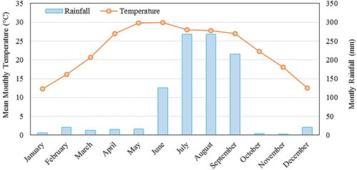
The study area is Nandhaur landscape (Figure 1), located in the lesser Himalayan region of Uttarakhand, India. It covers about 352 km² and is completely covered with deciduous as well as mixed deciduous forests from the lower foothills starting at 300 m asl to the ridge in 1000 m asl. The area is a crucial part of Terai Arc Landscape and encompasses about 170 km² area of Nandhaur Wildlife Sanctuary. The climate is of sub-tropical moist monsoon type. The monthly average temperature varies from 12 °C in January to 30 °C in June. Approximately 85% of the annual rainfall is concentrated during the rainy season. The rainy season is warm and wet (mid-June–September) while the winter and summer are cool-dry (November–February) and hot-dry (April–June), respectively (Figure 2).

Figure 1. Location map of the study area (i.e. Nandhaur Landscape). Field inventory plots location are overlaid on false colour composite of Sentinel-2 (R: NIR, G: Red, B: Green) image dated 8th December, 2018.

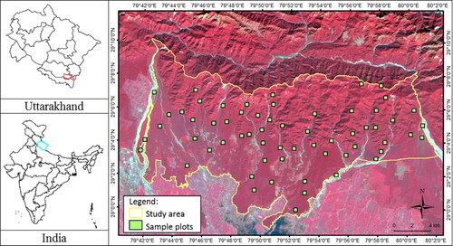
Figure 2. Ombrothermic diagram of mean temperature and monthly rainfall of the study area (Source: Eddy Covariance Flux Tower Site, Haldwani-http://asiaflux.net/index.php?page_id=61).

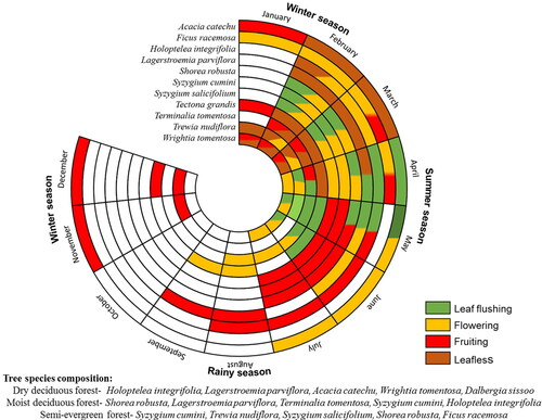
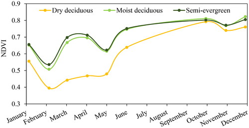
As per Champion and Seth (1968), tropical moist deciduous, tropical dry deciduous and tropical semi-evergreen are the main forest types in the study area. Owing to diverse habitat types, the area possesses high tree species richness (80 species). The landforms with shallow substrates is occupied by the dry deciduous forest dominate by Holoptelea integrifolia and Lagerstroemia parviflora. The moist deciduous forests are dominated by Shorea robusta which is associated with. Terminalia tomentosa, Syzygium cumini and Lagerstroemia parviflora. The semi-evergreen forest is confined to the riparian zones and is characterized by the presence of Syzygium cumini, Trewia nudiflora, Syzygium salicifolium and Ficus racemosa. These dominant tree species show high variation in leaf flushing phases during April and May (Figure 3). In tropical seasonal forest of India, in general, the leaf initiation begins in March with a peak in May before pre-monsoon showers (Elliott et al. 2006; Yadav and Yadav 2008; Nanda et al. 2014).

Figure 3. Asynchrony in phenological phases of the dominant trees (Dominance based on Important Value Index (IVI)) of different forest type.

2.2. Field sampling design and data analysis

The scientific survey of tree species in the Nandhaur region is very challenging due to the complex topography and dense forest cover. Under the Department of Biotechnology (DBT), Govt. of India funded project, this region has been earmarked for intensive exploration of phyto-diversity between 2018 and 2022. The research plots have been laid following the inventory protocol recommended by the Centre for Tropical Forest Science (CTFS) (https://www.ctc-n.org/resources/center-tropical-forest-science-ctfs).

A total of 61 field sample plots of 0.1 ha (31.6 × 31.6 m) were laid, representing all three forest types and microclimatic conditions meeting the criteria of saturation of the species-area curves. To determine the location for laying the field sample plots (Figure 1), three spatial layers representing the variations in forest type, elevation and moisture regime were used. ALOS 30-m spatial resolution Digital Elevation Model (DEM) prepared by the Japan Aerospace Exploration Agency (JAXA) (https://www.eorc.jaxa.jp/ALOS/en/aw3d30/) was used to derive topographical variables viz., elevation, slope, aspect and Topographic Wetness Index (TWI). We first considered the forest type map resulting in three strata, and further, both elevation and TWI map were grouped into 3 levels each resulting in a total of 27 strata. At least 2 plots were laid in each stratum while additional plots were laid in the lower elevation strata in proportion to area coverage. The location of each plot was recorded with a GPS (Spectra Precision MobileMapper 50) with better than 3m accuracy. The identification of unknown tree species was done by referring to herbarium of Botanical Survey of India (BSI), Dehradun.

Species diversity at the plot level was analysed using Shannon-Wiener diversity index (H'). H' is one of the most widely used diversity index that is sensitive to rarity and species abundance. H' was calculated for all tree species in each plot using the formula defined in Equation (1)(1) $$H\prime =\mathrm{ }-{\sum }_{i=1}^s{p}_{i}ln\mathrm{ }{p}_i$$(1) (Shannon and Weaver 1949): (1) $$H\prime =\mathrm{ }-{\sum }_{i=1}^s{p}_{i}ln\mathrm{ }{p}_i$$(1) where s is the total number of species and p_i is the proportion of species s made up of the ith species in the sample.

The plot level H' was used to relate satellite-derived SVH products. The plot-level tree H' was estimated considering the species with individuals of GBH (girth at breast height) ≥30 cm and for GBH < 30.

The dominant tree species of each forest type were identified based on importance value index (IVI) (Curtis and Cotton 1956). The seasonal leaf exchange behaviour of uppermost dominant tree species of each forest type during the dry and wet seasons is depicted for the study area (Figure 3). The IVI was calculated based on Equation (2)(2) $$\mathrm{IVI}=\text{ Relative frequency}+\text{Relative dominance}+\text{Relative density}$$(2) : (2) $$\mathrm{IVI}=\text{ Relative frequency}+\text{Relative dominance}+\text{Relative density}$$(2)

2.3. Satellite datasets

The MultiSpectral Instrument Level-1C (MSI L1C) imagery of Sentinel 2 A & 2B of the study area for 2018 was downloaded from Copernicus Open Access Hub (https://scihub.copernicus.eu/dhus/#/home). A total of nine cloud-free images of each month were downloaded except for July–September period due to unavailability of cloud-free images (Table 1). The downloaded images were pre-processed and atmospherically corrected using Sen2Cor (2.05.05-win64) plugin in SNAP. All the bands of corrected surface reflectance images were then resampled to 10 m. NDVI (Rouse et al. 1973) was calculated using band 4 (665 nm, Red) and band 8 (842 nm, NIR) (Equations 3(3) $$\mathrm{NDVI}=\frac{\mathrm{Band}\mathrm{ }8\mathrm{ }\left(842\mathrm{ }\mathrm{nm}\right)-\text{ Band }4\left(665\mathrm{ }\mathrm{nm}\right)}{\mathrm{Band}\mathrm{ }8\mathrm{ }\left(842\mathrm{ }\mathrm{nm}\right)+\text{ Band }4\left(665\mathrm{n}\mathrm{m}\right)}$$(3) ). (3) $$\mathrm{NDVI}=\frac{\mathrm{Band}\mathrm{ }8\mathrm{ }\left(842\mathrm{ }\mathrm{nm}\right)-\text{ Band }4\left(665\mathrm{ }\mathrm{nm}\right)}{\mathrm{Band}\mathrm{ }8\mathrm{ }\left(842\mathrm{ }\mathrm{nm}\right)+\text{ Band }4\left(665\mathrm{n}\mathrm{m}\right)}$$(3)

Table 1. Sentinel-2 datasets used in the study.

Sl. No.	Satellite	Date of acquisition
1.	Sentinel-2A	22 January 2018
2.	Sentinel-2A	21 February 2018
3.	Sentinel-2B	18 March 2018
4.	Sentinel-2A	22 April 2018
5.	Sentinel-2B	7 May 2018
6.	Sentinel-2A	21 June 2018
7.	Sentinel-2B	4 October 2018
8.	Sentinel-2B	23 November 2018
9.	Sentinel-2A	18 December 2018

2.4. Derivation of spectral heterogeneity index

Rao’s Q index was derived from Sentinel-2 NDVI images following Rocchini et al. (2017). The non-vegetative and agricultural areas were masked out. The index measures the distance d_ij among pixel values of an image, and their relative abundance, calculated as per Equation (5)(5) $$Q_{rs}=\mathrm{ }{\sum }_{i=1}^{F-1}{\sum }_{j=i+1}^F{d}_{ij}\mathrm{*}{p}_i\mathrm{*}{p}_j$$(5) : (5) $$Q_{rs}=\mathrm{ }{\sum }_{i=1}^{F-1}{\sum }_{j=i+1}^F{d}_{ij}\mathrm{*}{p}_i\mathrm{*}{p}_j$$(5) where, $Q_{\mathrm{r}s}$ = Rao’s Q index applied to remote sensing data, $p$ = relative abundance of a pixel value in a selected plot image (F). $\mathrm{ }{d}_{ij}$ = spectral distance between the ith and jth pixel value, i = pixel i and j = pixel j.

For this study, simple Euclidean distance was used to calculate the spectral distance based on NDVI. A moving window of 3 × 3 pixels was applied to match the size of the field sample plots so that the value of the tree species diversity calculated at the plot level can be compared with the spectral variability index. The Rao’s Q index was calculated using the rasterdiv (https://CRAN.Rproject. org/package = rasterdiv) package in the R environment. The multi-dimensional Rao’s Q index was calculated using a combination of multi-temporal NDVI images. The multi-temporal models were built based on R² value between Rao’s Q index over the year and tree species diversity. The image combination for generating multi-dimensional Rao’s Q index based on order of correlation from high to low. The image with next highest correlation was kept combining with the multi-temporal model. The multi-temporal model with images of summer and winter months was also analysed.

To decouple the effects of in-situ species diversity and species stress conditions for estimating spectral diversity, we correlated Rao’s Q index derived from NDVI and tree species diversity with the moisture stress index (MSI) computed from Sentinel-2 data of the month which showed the highest correlation between SH and species diversity. We also analysed the annual trend of NDVI with the trend of the R² time series of Rao’s Q index over the year.

2.5. Validation of spectral variability metrics as proxy to Species Diversity

Relation between plot data-based H' and NDVI-based Rao’s Q index was established using simple linear regression. The performance of Rao’s Q index derived from NDVI images in estimating tree diversity was assessed and the changes in correlation between Rao’s Q index and in-situ H' within a year were analysed.

3. Results

The species richness of trees was observed highest in semi-evergreen (54 species) forest followed by moist-deciduous (41 species) and dry-deciduous (40 species) forests. The mean plot-level tree richness was highest for semi-evergreen forest (Table 2). The mean plot level H' was comparatively higher for dry-deciduous followed by moist-deciduous forests. H' computed considering individuals with GBH ≥ 30 cm did not show much difference with the H' computed for individuals with GBH < 30 cm. It was also observed that the average height of trees with GBH lower than 30 cm was approximately 3 m which generally forms under-canopy of the forest whereas average height of trees with GBH ≥ 30 cm was 10–13 m across the forests which represents the forest canopy.

Table 2. Variation in tree species diversity and richness of each forest type and IVI of dominant species.

Forest type and no. of plots	Mean and range of tree species richness at plot level	Overall tree richness	Tree species diversity (H') at plot level		Tree species diversity (H') range (GBH ≥ 30cm)	Dominant species and IVI
			Tree with GBH ≥ 30cm	Including Tree with GBH < 30cm
Dry deciduous forest (20)	6 (2-13)	40	1.43	1.52	0.48 − 2.12	Holoptelea integrifolia (50.78), Acacia catechu (24.26), Lagerstroemia parviflora (20.65), Tectona grandis (18.71), Haldina cordifolia (18.65)
Moist deciduous forest (22)	8 (3-13)	41	1.42	1.47	0.59 − 2.27	Shorea robusta (99.34), Mallotus philippensis (28.59), Syzygium cumini (22.45), Terminalia tomentosa (14.21), Holoptelea integrifolia (12.46)
Semi-evergreen forest (19)	8 (3-14)	54	1.4	1.42	0.45 − 1.89	Syzygium cumini (68.5), Mallotus philippensis (42.78), Shorea robusta (20.91), Trewia nudiflora (14.19), Cordia myxa (12.98)

3.1. Relation between Rao’s Q index and H'

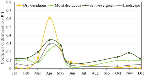
The temporal variation in the coefficient of determination (R²) between H' and Rao’s Q indices derived using Sentinel-2 NDVI showed a higher value during spring and summer seasons (Figure 4). A lower positive correlation was observed for monsoon and winter seasons. The highest R² value was observed in the month of April for the dry deciduous (R²-0.61) and semi-evergreen (R²-0.35) forest types, while in the moist deciduous forest highest correlation was observed in May (R²-0.28). The correlation for moist deciduous and semi-evergreen forest types showed comparatively less variation over the course of a year than the dry deciduous forest. At the landscape level, R² was comparatively lower throughout the year than individual forest types.

Figure 4. Temporal variation of R² between tree diversity (H') and Rao’s Q index based on NDVI for different forest types and the overall landscape (all forest type combined) over the year.

3.2. Multi-temporal spectral heterogeneity and correlation with H'

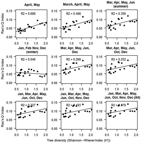
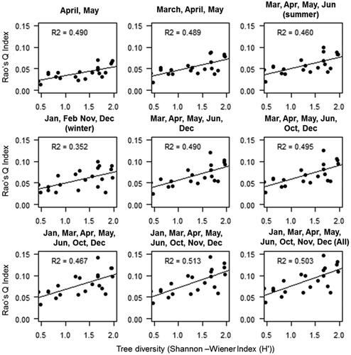
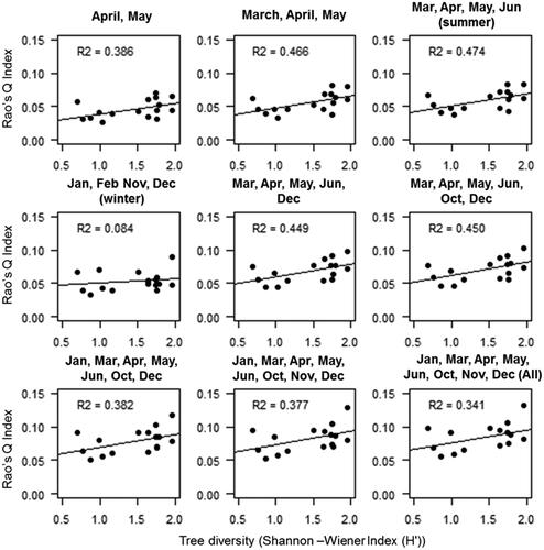
The multi-dimensional Rao’s Q index was calculated using multi-temporal NDVI images. Overall higher correlation was observed between H' and multi-dimensional Rao’s Q index. The use of multiple images increased the correlation between H' and Rao’s Q index up to a level beyond which the correlation tends to decline (Table 3).

Table 3. NDVI based Multi-temporal SVH models developed for different types.

Sl. No.	SVH Models	Months	Relation between tree diversity (H') and multi-temporal Rao’s Q index
			Dry deciduous	Moist deciduous	Semi-evergreen
1.	Model−1	April, May	0.688	0.490	0.386
2.	Model-2	March, April, May	0.488	0.489	0.466
3.	Model-3	March, April, May, June (Summer months)	0.356	0.460	0.474
4.	Model-4	January, February, November, December (Winter months)	0.046	0.352	0.084
5.	Model-5	March, April, May, June, December	0.268	0.490	0.449
6.	Model-6	March, April, May, June, October, December	0.252	0.495	0.450
7.	Model-7	January, March, April, May, June, October, December	0.227	0.467	0.382
8.	Model-8	January, March, April, May, June, October, November, December	0.193	0.513	0.377
9.	Model-9	All images	0.179	0.503	0.341

3.2.1. Dry deciduous forest

Rao’s Q index derived using all 9 months NDVI images showed a lower correlation with H' (R² 0.179, Figure 5). The highest R² value (0.688) was observed using two images of April and May and significant variation in R² was found with increasing the number of images. The inclusion of images other than the growing season significantly lowered the correlation for dry deciduous forest type. The Rao’s Q index derived using only winter images showed the least correlation (R² = 0.046) with H'.

Figure 5. Relation between tree diversity (H') and NDVI derived multi-dimensional Rao’s Q index for Dry deciduous forest.

3.2.2. Moist deciduous forest

For moist deciduous forests, the highest R² values (0.513) were observed using eight-month images of January, March, April, May, June, October, November and December which slightly decrease (0.503) while using all images (Figure 6). The moist deciduous forest showed lower variation in R² than dry deciduous forest which ranged from 0.352 for winter month images to 0.513 for eight date images.

Figure 6. Relation between tree diversity (H') and NDVI derived multi-dimensional Rao’s Q index for Moist deciduous forest.

3.2.3. Semi-evergreen forest

The highest correlation (R² 0.47) for semi-evergreen forests was observed using four images (Figure 7), while the lowest (0.084) was for winter month images. The semi-evergreen forest also showed low variation in R². Among the forest types, semi-evergreen forests observed the lowest R² value.

Figure 7. Relation between tree diversity (H') and NDVI derived multi-dimensional Rao’s Q index for Semi-evergreen forest.

Rao’s Q index and H' did not show any significant correlation with the MSI for any of the three forest types (Figure 8). On analysing the trend of NDVI with the trend of R² of H' and Rao’s Q index, it was observed that the R² was higher when the NDVI started rising from its lowest point (Figure 9). The lowest NDVI was observed in February after which it started increasing up to the post-monsoon months. However, there is a slight dip in NDVI in May for moist deciduous and semi-evergreen forests.

Figure 8. Relation of tree diversity (H') and Rao’s Q index derived from NDVI with Moisture Stress Index (MSI) of Sentinel-2 (22 April, 2018 for dry- & moist deciduous and 7 May, 2018 for Semi-evergreen forest).

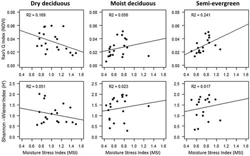
Figure 9. Annual trend of NDVI computed from Sentinel-2 for different forest types.

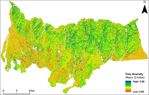
3.3. Spatial pattern of Rao’s Q diversity index

The spatial pattern of Rao’s Q index was mapped using combined multi-date NDVI images which showed highest coefficient of determination with H' for each forest type (Figure 10). The regression equation of the best regression models for semi-evergreen, dry and moist-deciduous forests was y = 0.0184x + 0.0325, y = 0.0351x + 0.0138, and y = 0.0383x + 0.0338, respectively. Higher value of Rao’s Q index was observed for upper mountainous region which is also part of the Nandhaur Wildlife Sanctuary while the lower foothills and flat terrains outside the protected area showed lower Rao’s Q index. Overall, the multi-dimension Rao’s Q index performed well to capture the pattern of diversity over the study area.

Figure 10. Composite Rao’s Q index-based tree diversity map at 0.1 ha scale derived from multi-date NDVI.

4. Discussion

During the past two decades, several attempts have been made to estimate plant diversity based on SVH using satellite images by applying different SH indices (Palmer et al. 2002; Torresani et al. 2018; Khare et al. 2019; Rocchini et al. 2017). This has extended the applicability of SVH to estimate species diversity over several ecosystems. Considering the typical phenological regime of tropical seasonal forests, this study assessed the tree diversity of tropical seasonal forests by thoroughly analysing Rao’s Q index derived from NDVI over the year at landscape level. The study was conducted in Nandhaur landscape which maintains a very high canopy cover across all forest types owing to the status of a Wildlife Sanctuary and hence, maximum contribution to plot level tree diversity came from canopy forming species.

This study showed a significant correlation between NDVI-derived Rao’s Q index and H' measurement suggesting that the estimation of tree species diversity in tropical seasonal forests could be done using satellite images. The seasonal differences in vegetation traits across tree species cause variability in NDVI. Hence, it was not surprising that the statistical relationship between Rao’s Q index and H' also varied throughout the year. Similarly, Madonsela et al. (2017) and Rocchini et al. (2019) have reported that the spectral variability between tree species depends on the time of image acquisition. The intra-annual R² trend is driven by the typical variation of NDVI due to phenology instead of the change in tree species diversity that remains relatively stable. The heterogeneity of NDVI at specific times of the year reflects the phenological heterogeneity that is linked to the tree species diversity of tropical seasonal forests (Torresani et al. 2019).

In general, Rao’s Q index showed the highest relationship (R²) with the in-situ tree species diversity in summer when the NDVI time series curve begins to rise from its lowest point, whereas a lower correlation was observed during winter. Previous studies have also reported stronger relationships during the leaf initiation period, while the weaker relationship were recorded during the senescence period in other ecosystems (Arekhi et al. 2017; Torresani et al. 2019). This may be attributed to larger spectral variation pertaining to phenological variation among the tree species during the leaf initiation period (spring-summer season) as no significant correlation between MSI and spectral diversity was observed. Moist deciduous tree species of dry monsoon forests in India form new leaves almost 1–2 months prior to the first monsoon rains, during the hottest and driest part of the year(Elliott et al. 2006; Yadav and Yadav 2008; Nanda et al. 2014). Among the 10 most dominant tree species in the study area, leaf flush or leaf initiation becomes pronounced from April (6 species) and peaks in May (8 species) in the dry season for species such as Acacia catechu, Holoptelia integrefolia and Lagerstroemia parviflora. Hence, showing a higher correlation during this period. Whereas during post-monsoon, a lower correlation was observed when NDVI reached the highest. This could be due to the fact NDVI saturates over high chlorophyll content and is unable to capture small variations in reflectance due to changes in leaf pigments, which tend to be more gradual within landscapes (Steele et al. 2008; He et al. 2009).

Phenology remarkably affects the visual, biochemical and biophysical properties of the seasonal forests, though the strength of these dynamics may differ across the regions. Hence vegetation belonging to distant habitats and environmental regimes would show different relationships between H' and SH. This study demonstrated that Rao’s Q index has lower correlation with H' for the entire landscape but corresponds well with individual forest types, an observation similar to Schmidtlein and Fassnacht (2017). The magnitude and timing of Rao’s Q index’s relation with H' were observed differently for each forest type. The dry deciduous forest observed the highest R² between Rao’s Q index and H' followed semi-evergreen forest. The moist deciduous forest observed the lowest R² and also showed the lowest variation in R² over the year which may due to the fact the moist deciduous forest in the study area is mostly dominated by Sal, with the highest relative dominance up to 90%. However, the dry deciduous and semi-evergreen forest are more heterogeneous with several deciduous tree species shedding leaves during winter months. The spring-to-summer transition period in these forests offered higher spectral variability compared to other seasons.

The study also highlighted that the multi-dimensional Rao’s index evaluated using multi-temporal NDVI images showed better correlation with H' than Rao’s Q index evaluated using a single date image. This may be because multi-temporal images can record a range of the phenological changes and leaf traits of different tree species, thus increasing the spectral separability amongst them (Hill et al. 2010; Chrysafis et al. 2020). The higher correlation was found in the summer season for dry deciduous and semi-evergreen forest while moist deciduous forest showed the highest correlation when all images except for one image of February was used for Rao’s Q index. The canopy of moist deciduous forest in the study area is dominated by Sal which start shedding leaves in a relatively brief period in February with concentrated leaf-fall in March synchronous with leaf-flushing showing a leaf-exchanging pattern (Newton, 1988). In general, increasing multi-temporal images to estimate tree diversity in homogenous or gregarious forest type would increase the correlation. However, inclusion of images of senescence period might slightly drop the correlation.

The dry deciduous forests observed the highest R² for April and May image, due to higher variation in phenology between tree species during the early growing season. While the semi-evergreen forest observed the highest correlation when four summer images of March, April, May and June were used. However, February month images observed the highest exposure of tree stems when most of the trees are in leafless conditions, which on the contrary observed a very low correlation between Rao’s Q index and field plot diversity. With leaf flushing in March, the spectral variability increases and hence, Rao’s Q index relation with H' also increased. The dry deciduous forest shows sharp leaf initiation causing a higher correlation with two multi-temporal images of summer to get better correlation while the semi-evergreen forest required more temporal images of summer. Beside the differences in foliage, species differ in terms of canopy architecture (branching pattern) and stems (bark surface), hence, increase in SH on this account could positively contribute to tree diversity estimation.

Since the study found the performance of Rao’s Q index differs according to the type of forest, composite map was prepared by combining the Rao’s Q index maps of each forest type to represent the landscape scale tree diversity. The northern and north-western aspects and stream courses in the Lesser Himalayan mountain ranges store more moisture as compared to the south and southeast aspects, supporting a greater diversity of species. The composite landscape-level tree diversity map derived in this study well explains this phenomenon. Most of the hilly parts of the Nandhaur landscape that comes under wildlife sanctuary are protected from biotic disturbance and showed higher tree diversity as compared to the region outside the protected area. It also emphasizes that the index is sensitive to the gregarious nature of forests and has negative effects of biotic disturbances on tree diversity in the peripheral areas of the sanctuary.

This study developed an approach that explores the multi-temporal NDVI of Sentinel-2 to estimate spatial tree diversity patterns at landscape level. The free availability of multi-temporal and multi-spectral Sentinel-2 data enables researchers to explore its applicability for larger landscapes. The NDVI-based SVH model developed in this study can be scaled to the entire Terai Arc Landscape, of similar vegetation composition, for regional scale tree diversity hotspot identification and monitoring biodiversity changes.

5. Conclusions

The use of Rao’s Q index is a promising method for estimating species diversity using satellite remote sensing images. This study suggests an approach to improve Rao’s Q index’s applicability to seasonal tropical forests. The proposed method is advantageous in the following ways: (i) determining the optimal time for Rao’s index to perform best in estimating diversity; (ii) recommending the use of multiple dimensional Rao’s Q index greatly enhances its relationship with measured tree diversity since it incorporates the phenological variability; and (iii) the performance of Rao’s index significantly differs between forest types, the landscape-scale diversity has to be examined by combining the diversity index generated for the distinct forest type. Based on the encouraging results of this study, it is suggested that Rao’s Q index based on Sentinel-2's multi-temporal NDVI should be used for tree diversity estimation for different seasonal ecosystems.

Acknowledgements

The research presented in this article was carried out under the project "Biodiversity Characteristics at Community Level using EO data" funded by the Department of Biotechnology (DBT) and Department of Space (DOS), Government of India. The authors are thankful to the European Space Agency (ESA) for Sentinel-2 data and the Uttarakhand Forest Department for providing support in field data collection. We also thank the Director and Dean of the Indian Institute of Remote Sensing (IIRS), Dehradun for the encouragement and logistics facilities.

Disclosure statement

The authors declare that they have no known competing financial interests or personal relationships that could have appeared to influence the work reported in this paper.

Additional information

Funding

This work was jointly funded by the Department of Biotechnology (DBT), New Delhi and the Department of Space (DOS), Bengaluru.

References

- Arekhi M, Yılmaz OY, Yılmaz H, Akyüz YF. 2017. Can tree species diversity be assessed with Landsat data in a temperate forest? Environ Monit Assess. 189(11):1–14.
- Carlson KM, Asner GP, Hughes RF, Ostertag R, Martin RE. 2007. Hyperspectral remote sensing of canopy biodiversity in Hawaiian lowland rainforests. Ecosystems. 10(4):536–549.
- Champion HG, Seth SK. 1968. A revised survey of the forest types of India. Nasik: Government of India Press; p. 404.
- Chiarucci A, Bacaro G, Scheiner SM. 2011. Old and new challenges in using species diversity for assessing biodiversity. Philos Trans R Soc Lond B Biol Sci. 366(1576):2426–2437.
- Chrysafis I, Korakis G, Kyriazopoulos AP, Mallinis G. 2020. Predicting tree species diversity using geodiversity and sentinel-2 multi-seasonal spectral information. Sustainability. 12(21):9250.
- Curtis JT, Cotton G. 1956. Plant ecology workbook, laboratory field manual. Minnesota (MN): Burgess Publishing; p. 193.
- Draper FC, Baraloto C, Brodrick PG, Phillips OL, Martinez RV, Honorio Coronado EN, Baker TR, Zárate Gómez R, Amasifuen Guerra CA, Flores M, et al. 2019. Imaging spectroscopy predicts variable distance decay across contrasting Amazonian tree communities. J Ecol. 107(2):696–710.,
- Elliott S, Baker PJ, Borchert R. 2006. Leaf flushing during the dry season: the paradox of Asian monsoon forests. Glob Ecol Biogeograph. 15(3):248–257.
- Féret JB, Asner GP. 2014. Mapping tropical forest canopy diversity using high‐fidelity imaging spectroscopy. Ecol Appl. 24(6):1289–1296.
- Gould W. 2000. Remote sensing of vegetation, plant species richness, and regional biodiversity hotspots. Ecol Appl. 10(6):1861–1870.
- He KS, Zhang J, Zhang Q. 2009. Linking variability in species composition and MODIS NDVI based on beta diversity measurements. Acta Oecol. 35(1):14–21.
- Hill SL, Harfoot M, Purvis A, Purves DW, Collen B, Newbold T, Burgess ND, Mace GM. 2016. Reconciling biodiversity indicators to guide understanding and action. Conserv Lett. 9(6):405–412.
- Hill RA, Wilson AK, George M, Hinsley SA. 2010. Mapping tree species in temperate deciduous woodland using time-series multi-spectral data. Appl Veg Sci. 13(1):86–99.
- Janzen DH. 1988. Tropical dry forests. Biodiversity. 15:130–137.
- Khare S, Latifi H, Rossi S. 2019. Forest beta-diversity analysis by remote sensing: how scale and sensors affect the Rao’s Q index. Ecol Indic. 106:105520.
- Levin N, Shmida A, Levanoni O, Tamari H, Kark S. 2007. Predicting mountain plant richness and rarity from space using satellite‐derived vegetation indices. Div Distribut. 13(6):692–703.
- Lopes M, Fauvel M, Ouin A, Girard S. 2017. Spectro-temporal heterogeneity measures from dense high spatial resolution satellite image time series: application to grassland species diversity estimation. Remote Sens. 9(10):993.
- Madonsela S, Cho MA, Ramoelo A, Mutanga O. 2017. Remote sensing of species diversity using Landsat 8 spectral variables. ISPRS J Photogramm Remote Sens. 133:116–127.
- Nanda A, Suresh HS, Krishnamurthy YL. 2014. Phenology of a tropical dry deciduous forest of Bhadra wildlife sanctuary, southern India. Ecol Process. 3(1):1–12.
- Newton PN. 1988. The structure and phenology of a moist deciduous forest in the Central Indian Highlands. Vegetation. 75(1–2):3–16.
- Pereira HM, Ferrier S, Walters M, Geller GN, Jongman RHG, Scholes RJ, Bruford MW, Brummitt N, Butchart SHM, Cardoso AC, et al. 2013. Essential biodiversity variables. Science. 339(6117):277–278.,
- Palmer MW, Wohlgemuth T, Earls P, Arévalo JR, Thompson SD. 2000. Opportunities for long-term ecological research at the Tallgrass Prairie Preserve, Oklahoma. In: Lajtha K,Vanderbilt K, editors. Cooperation in Long Term Ecological Research in Central and Eastern Europe: proceedings of ILTER Regional Workshop; 22–25 June, 1999; Budapest, Hungary. Oregon State University: Corvallis p. 123–128.
- Palmer MW, Earls PG, Hoagland BW, White PS, Wohlgemuth T. 2002. Quantitative tools for perfecting species lists. Environmetrics. 13(2):121–137.
- Rocchini D, Chiarucci A, Loiselle SA. 2004. Testing the spectral variation hypothesis by using satellite multispectral images. Acta Oecol. 26(2):117–120.
- Rocchini D, Marcantonio M, Ricotta C. 2017. Measuring Rao’s Q diversity index from remote sensing: an open source solution. Ecol Indic. 72:234– 238.
- Rocchini D, Luque S, Pettorelli N, Bastin L, Doktor D, Faedi N, Feilhauer H, Féret J‐B, Foody GM, Gavish Y, et al. 2018. Measuring β‐diversity by remote sensing: a challenge for biodiversity monitoring. Methods Ecol Evol. 9(8):1787–1798.,
- Rocchini D, Marcantonio M, Da Re D, Chirici G, Galluzzi M, Lenoir J, Ricotta C, Torresani M, Ziv G. 2019. Time-lapsing biodiversity: an open source method for measuring diversity changes by remote sensing. Remote Sens Environ. 231:111192.
- Rouse JW, Haas RH, Schell JA, Deering DW. Jr 1973. Monitoring the vernal advancement and retrogradation (green wave effect) of natural vegetation (No. NASA-CR-132982).
- Schmidtlein S, Fassnacht FE. 2017. The spectral variability hypothesis does not hold across landscapes. Remote Sens Environ. 192:114–125.
- Shannon CE, Weaver W. 1949. The mathematical theory of communication. Champaign (IL): University of Illinois, Urbana; p. 117.
- Skidmore AK, Pettorelli N, Coops NC, Geller GN, Hansen M, Lucas R, Mücher CA, O'Connor B, Paganini M, Pereira HM, et al. 2015. Environmental science: agree on biodiversity metrics to track from space. Nature. 523(7561):403–405.,
- Slik JWF, Arroyo-Rodríguez V, Aiba S-I, Alvarez-Loayza P, Alves LF, Ashton P, Balvanera P, Bastian ML, Bellingham PJ, van den Berg E, et al. 2015. An estimate of the number of tropical tree species. Proc Natl Acad Sci USA. 112(24):7472–7477.
- Steele M, Gitelson AA, Rundquist D. 2008. Nondestructive estimation of leaf chlorophyll content in grapes. Am J Enol Vitic. 59(3):299–305.
- Torresani M, Rocchini D, Zebisch M, Sonnenschein R, Tonon G. 2018. Testing the spectral variation hypothesis by using the RAO-Q index to estimate forest biodiversity: effect of spatial resolution. IGARSS 2018-2018 IEEE International Geoscience and Remote Sensing Symposium; Valencia, Spain. July. Piscataway (NJ): IEEE; p. 1183–1186.
- Torresani M, Rocchini D, Sonnenschein R, Zebisch M, Marcantonio M, Ricotta C, Tonon G. 2019. Estimating tree species diversity from space in an alpine conifer forest: the Rao’s Q diversity index meets the spectral variation hypothesis. Ecol Inf. 52:26–34.
- Torresani M, Rocchini D, Sonnenschein R, Zebisch M, Hauffe HC, Heym M, Pretzsch H, Tonon G. 2020. Height variation hypothesis: a new approach for estimating forest species diversity with CHM LiDAR data. Ecol Indic. 117:106520.
- Torresani M, Feilhauer H, Rocchini D, Féret JB, Zebisch M, Tonon G. 2021. Which optical traits enable an estimation of tree species diversity based on the Spectral Variation Hypothesis? Appl Veg Sci. 24(2):e12586.
- Yadav RK, Yadav AS. 2008. Phenology of selected woody species in a tropical dry deciduous forest in Rajasthan, India. Trop Ecol. 49(1):25.