Identifying inter-seasonal drought characteristics using binary outcome panel data models

Abstract

This study mainly focuses on spatiotemporal and inter-seasonal meteorological drought characteristics. Random Effect Logistic Regression Model (RELRM) and Conditional Fixed Effect Logistic Regression Model (CFELRM) are used to identify the spatiotemporal and inter-seasonal characteristics of meteorological drought in selected stations. The log-likelihood Ratio Chi-Square (LRCST) and Wald chi-square tests (WCTs) are used to assess the significance of RELRM and CFELRM. The Hausman test (HT) is applied to select the appropriate model between RELRM and CFELRM. For instance, HT suggests the CFELRM as an appropriate model in spring-to-summer spatiotemporal drought modelling. The significant coefficient from CFELRM indicates that an increment in moisture conditions of the spring season will decrease the probability of drought in the summer. The odds ratio of 0.1942 means that 19.42% chance of being in a higher category. Similarly, in summer-to-autumn using RELRM the computed odds ratio of 0.0673 shows that 6.73% chance of being in a higher category.

Keywords:

• Standardized drought indices
• meteorological drought
• drought persistence
• Conditional Fixed Effect Logistic Regression Model
• random effect logistics model

1. Introduction

Drought is the greatest recurring natural hazard and becomes a source of huge losses in agriculture sectors (Cunha et al. 2019; Mondol et al. 2021; Ha et al. 2022; Orimoloye et al. 2022; Zarei et al. 2023), natural ecosystems (Deng et al. 2021; Yao et al. 2022) and forestry (Anderegg et al. 2020; Sánchez-Pinillos et al. 2022). Its impacts slowly hold an area over time, and it may remain for a long phase; in severe instances, drought can be sustained for many years and distress the environment, agriculture and socio-economic sectors (Haile et al. 2020; Chen et al. 2021; Han and Yang 2021; Jordaan 2022; Savelli et al. 2022; Sharma and Sen 2022). The researchers have broadly segregated the drought into numerous classes, i.e. meteorological, agricultural, hydrological and socio-economic (Bae et al. 2019; Ding et al. 2021; Satoh et al. 2021; Arabameri et al. 2022; Vicente-Serrano et al. 2022). Quiring (2009) defined meteorological drought as a deficiency of precipitation (or moisture supply) over some time. Numerous studies use precipitation data to analyse meteorological drought (Adib and Marashi 2019; Spinoni et al. 2019; Guo et al. 2020). The streamflow data is frequently used for studying hydrological drought (Lee et al. 2015; Salimi et al. 2021; Tareke and Awoke 2022). The socio-economic drought is connected to a shortfall in water resources systems and the water supply being unable to meet water demands. Drought has multifaceted dynamics in various fields; and therefore, effective drought monitoring and prediction procedures are required to explain the crucial dynamics to manage and mitigate the effects of droughts (Vogt and Somma 2013; Solh and van Ginkel 2014; Hassan et al. 2019). Various studies have developed several procedures for assessing and monitoring drought phenomena (Kim and Jehanzaib 2020; Niaz, Hussain, Ali, et al. 2021e; Niaz, Almazah, Hussain, et al. 2021; Aadhar and Mishra 2022; Alahacoon and Edirisinghe 2022; Lotfirad et al. 2022; Prodhan et al. 2022; Niaz, Tanveer, et al. 2022).

Recently, several studies have introduced a variety of drought indices to investigate drought more precisely (Esfahanian et al. 2017; Yang et al. 2018; Adib and Tavancheh 2019; Yihdego et al. 2019; Afshar et al. 2022; Niaz, Iqbal, et al. 2022; Niaz, Almazah, Al-Duais, et al. 2022). The drought indices are used for quantifying different kinds of droughts (meteorological, hydrological and agricultural) (Keyantash and Dracup 2004; Kao and Govindaraju 2010; Mishra and Singh 2010, 2011; ZargaR et al. 2011; Surendran et al. 2017). Palmer (1965) introduced (PDSI), for measuring the cumulative departure of moisture supply. The PSDI relates to the water supply instead of precipitation irregularity. It includes varying indicators, including temperature, precipitation and soil data. The PDSI computes evapotranspiration, moisture, soil recharge and runoff based on these indicators as inputs. Svoboda et al. (2002) proposed US Drought Monitor (USDM). The USDM is frequently used in the US. The use of the USDM is high at the organizational level for research. The Standardized Precipitation Index (SPI) was developed by McKee et al. (1993). The standardized Precipitation Evapotranspiration Index (SPEI) was developed by (Vicente-Serrano et al. 2010) and comprises the effect of temperature variability in drought evaluation. Several studies used SPEI for drought assessment (Zhao et al. 2017; Li et al. 2020; Zarei and Mahmoudi 2020; Mokhtar et al. 2021; Masanta and Srinivas 2022; Niaz, Almazah, Hussain, Faisal, et al. 2022; Niaz, Almazah, Hussain, Filho, et al. 2022) and standardized precipitation and temperature Index (SPTI) by (Ali et al. 2017). Among the various meteorological indices, the SPI is famous for defining meteorological drought. The SPI is based only on precipitation data. The simplicity in calculation and ability to assess drought for different time scales, therefore, is renowned and used in several studies for the assessment, monitoring and forecasting of drought events (Naresh Kumar et al. 2009; Türkeş and Tatlı 2009; Angelidis et al. 2012; Stagge et al. 2015; Cerpa Reyes et al. 2022; Elbeltagi et al. 2023). ; SPI can be deployed for longer scales to reflect the agricultural and hydrological drought. For instance, the SPI for a nine-month time scale with a value of less than −1.5 is the best indication of an agricultural drought (ZargaR et al. 2011). The SPI value at the twelve-month time scale can reflect the streamflow, reservoir level, etc.

Drought early warning and monitoring are crucial to drought preparedness and mitigation plans. Several studies have used frameworks to monitor and predict drought occurrences in different climatic conditions (Nayak and Hassan 2021; Niaz, Hussain, Zhang, et al. 2021; Alawsi et al. 2022; Dikshit et al. 2022). Linear regression is a traditional approach used for statistical prediction (Güner Bacanli 2017; Kim et al. 2020; Papadopoulos et al. 2021). Generally, these regression models mainly deal with the continuous dependent variable. The linear regression models cannot perform appropriately for the categorical dependent variable. Therefore, categorical-based frameworks are commonly developed, for example, logistic regression, multiple logistic regression, ordered logistic regression, etc. (Ford and Labosier 2014; Bachmair et al. 2017; Meng et al. 2017; Niaz, Zhang, et al. 2021; Niaz, Tanveer, et al. 2022). Ford and Labosier (2014) used logistic regression to find drought persistence in varying stations. Meng et al. (2017) used logistic regression for the categorical dependent variable to find the spatial pattern of drought. Niaz, Raza, et al. (2022) recently used a proportional odds model to find inter-seasonal drought characteristics in various stations. However, these studies have not addressed the spatiotemporal effect of meteorological drought. The spatiotemporal and inter-seasonal drought characteristics can implicitly support reducing the potential negative impacts of drought. Therefore, finding the spatiotemporal characteristics of meteorological drought for prediction is vital. Thus, this issue underpins the development of the new methodology. Therefore, the current research examines spatiotemporal drought characteristics in numerous seasons (winter, spring, summer and autumn). The binary outcome panel data models with Random Effect Logistic Regression Model (RELRM) and Conditional Fixed Effect Logistic Regression Model (CFELRM) are utilized for identifying the spatiotemporal and inter-seasonal drought characteristics. Further, to substantiate the significance of RELRM and CFELRM for the seasonal investigations, the log-likelihood Ratio Chi-Square Test (LRCST) and Wald chi-square test (WCT) are utilized. The tests suggest that both models can be used for the current analysis. However, based on Hausman Test (HT), the more appropriate model is chosen to describe the spatiotemporal and inter-seasonal drought persistence. Moreover, the outcomes of the current analysis provide the groundwork for paying more attention to early warning systems for effectively managing water resources to avoid negative drought impacts in Pakistan.

2. Material and methods

2.1. Description of the study area

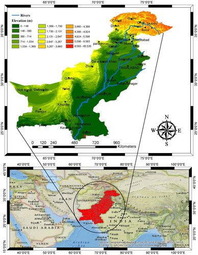
The geographic coordinates of Pakistan (Figure 1) are Latitude: 30° 23′ 21.84′′ N and Longitude: 69° 21′ 11.59′′ E covering a total area is 796,096 $\mathrm{k}{\mathrm{m}}^2.$ Due to domain variability, its climate changes as country topography, and it’s extremely exposed to the impact of climate change because of its geographical location, low technological resources, high population level, high internal variability and low resource base. The seasonal and annual rainfall patterns and extreme weather are changing, leading to droughts, landslides, cyclones and floods. In Pakistan, the winter and summer seasons often provide rain due to two primary meteorological phenomena: the summer monsoon from South Asia and the western parts. The average temperature reported by rainfall systems during monsoon and winter seasons is between 12 and 20 degrees Celsius and 19 and 35 degrees Celsius, respectively, and around 31 and 45% of the yearly rainfall during winter and monsoon seasons. Moreover, Pakistan has a semi-industrialized economy with a well-integrated agriculture sector. Most of the population of Pakistan is based on the agricultural sectors. Hence, the extreme drought events can be dangerous for agricultural sectors, ultimately affecting the country’s population. Drought is progressively threatening Pakistan’s agricultural and economic sectors (Anjum et al. 2012; Haroon et al. 2016; Waseem, Khurshid, et al. 2022; Hussain et al. 2023). Besides the ecological losses, drought can disturb the economy and negatively affect food security in the country (Idrees et al. 2022; Waseem, Jaffry, et al. 2022). Therefore, assessment and drought monitoring should be adequately executed to assist policymakers and water managers in improving drought management policies.

Figure 1. Geographical locations of selected stations.

2.2. Data and methods

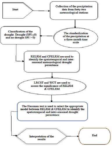
This research results are derived from the time-series data ranging from January 1971 to December 2017 for 42 meteorological stations in Pakistan. The climatological characteristics of the selected stations are suitable for current research. Therefore, the SPI at a three-month time scale (SPI-3) is utilized for the current analysis. For identification of the spatiotemporal and inter-seasonal drought characteristics in various stations, this study uses the binary outcome panel data models with RELRM and CFELRM. The LRCST and WCT are utilized to measure the significance of RELRM and CFELRM (Figure 2).

Figure 2. Framework for the application of binary panel data models.

2.2.1. Standardized precipitation index (SPI)

SPI has been widely used in assessing and monitoring drought for varying time scales (Angelidis et al. 2012; Stagge et al. 2015; Niaz, Almazah, Zhang, et al. 2021; Niaz, Hussain, Zhang, et al. 2021; Niaz, Zhang, et al. 2021; Cerpa Reyes et al. 2022; Elbeltagi et al. 2023). The calculation of the SPI is merely based on the precipitation observations. SPI can be used to compare drought events in different climate regions (Cunha et al. 2019; Mondol et al. 2021; Ha et al. 2022; Orimoloye et al. 2022). SPI is interrelated to the moisture deficit in the soil at short timescales, whereas it can be linked to the groundwater and reservoir at longer timescales (Cerpa Reyes et al. 2022; Kamali and Asghari 2022; Elbeltagi et al. 2023). Several techniques are used to standardize observed precipitation to quantify the SPI values (Naresh Kumar et al. 2009; Türkeş and Tatlı 2009; Farahmand and AghaKouchak 2015). However, in the current analysis, we adopted the transformation method (Farahmand and AghaKouchak 2015) of SPI is as follows, (1) $$\mathrm{SPI}=\mathrm{ }-\mathrm{ }(r-\mathrm{ }\frac{g_0+\mathrm{ }{g}_{1}r+\mathrm{ }{g}_2{r}^2}{1+\mathrm{ }{h}_{0}r+\mathrm{ }{h}_1{r}^2+\mathrm{ }{h}_2{r}^3})$$(1)

For $$r=\mathrm{ }\sqrt{\mathrm{l}\mathrm{n}\left[\frac{1}{{\left\{B\left(x\right)\right\}}^2}\right]}$$

For $B\left(x\right)$ (see, Farahmand and AghaKouchak 2015; Ali et al. 2020; Niaz, Tanveer, et al. 2022).

When (2) $$0\mathrm{ }\le \mathrm{ }B\left(x\right)\mathrm{ }\le 0.5$$(2) (3) $$\mathit{SPI}=\mathrm{ }+\mathrm{ }(r-\mathrm{ }\frac{g_0+\mathrm{ }{g}_{1}r+\mathrm{ }{g}_2{r}^2}{1+\mathrm{ }{h}_{0}r+\mathrm{ }{h}_1{r}^2+\mathrm{ }{h}_2{r}^3})$$(3)

And for $$r=\mathrm{ }\sqrt{\mathrm{l}\mathrm{n}\left[\frac{1}{{\{1-B\left(x\right)\}}^2}\right]}$$

When (4) $$0.5\le \mathrm{ }B\left(x\right)\mathrm{ }\le 1$$(4) where $g_0=2.515517,$ $g_1=0.802853,$ $g_2=0.010328,$ $h_0=1.432788,$ $h_1=0.189269,$ $h_2=0.001308.$

2.2.2. Binary response panel data modelling

Binary response modelling applies in several studies (Manski 1988; Sueyoshi 1995; Horowitz and Savin 2001; Kleinbaum and Klein 2010; Chauhan et al. 2016). Particularly use of panel data analysis is prominent in the literature (Honoré and Lewbel 2002; Arellano and Carrasco 2003; Sutradhar et al. 2008; Charbonneau 2017; Semykina and Wooldridge 2018). The panel model for binary response is given by, $$z_{it}^{\mathrm{*}}=x_{it}^{\prime }\beta +{\mu }_i+{\in }_{it}, \mathrm{i}=1,2,\mathrm{ }\dots ,\mathrm{ }\mathrm{n},\mathrm{ }\mathrm{t}=1,2,\mathrm{ }\dots ,\mathrm{ }\mathrm{T}.$$ $$z_{it}=1\mathrm{ }if\mathrm{ }{z}_{it}^{\mathrm{*}}>0,\text{ and zero otherwise}$$ z indicates the binary response, $i$ indicates the individual or items and $t$ indicates the number of observations within $i,$ which vary over time. $x$ indicates explanatory variables, $\beta$ is the regression coefficient, ${\mu }_i$ is the individual-specific effect and ${\in }_{it}$ is called idiosyncratic errors because these vary across $i$ as well as across $t.$ Ideally, we are interested in the correlation of ${\in }_{it}$ and ${\in }_{is}$ within the group but uncorrelated across the groups. ${\mu }_i$ is the unobserved individual-specific effect which vary across the groups. We decide between fixed and random effect models by examing the relationship between ${\mu }_i$ and ${ x}_{it}.$ The random effect model assumes that ${\mu }_i$ and ${ x}_{it}$ are not correlated, which also means that the conditional distribution of $f({\mu }_i|{ x}_{it})$ does not dependent on $x_{it}.$ If there is a correlation between ${\mu }_i$ and ${ x}_{it},$ then we prefer the fixed effect model.

2.2.3. Conditional fixed-effect logistic regression model

Conditional fixed-effect logistic regression gives us a consistent estimate as compared to unconditional fixed-effect logistic regression. The nonlinear binary response model is given by, (5) $$\mathit{prob}\left(z_{it}=1x_{it},{\mu }_i\right)=M(x_{it}\beta +{\mu }_i)$$(5)

The M is a nonlinear function; hence, we cannot use linear regression for estimating purposes. There are various nonlinear functions for estimating M in the literature, but the most common nonlinear function for M is the logit function. (6) $$M\left(x_{it}\beta +{\mu }_i\right)=\frac{e^{x_{it}\beta +{\mu }_i}}{1+e^{x_{it}\beta +{\mu }_i}}$$(6)

The range is between zero and one for the above function. This is also called a cumulative distribution function (CDF) for the logistic variable.

If M is the logistic CDF, then we obtain the log-likelihood as (7) $$\mathit{lnL}\left(zx;\beta \right)=\sum _{i=1}^N\{z_i\mathrm{l}\mathrm{n}(\frac{e^{x_{it}\beta +{\mu }_i}}{1+e^{x_{it}\beta +{\mu }_i}})+(1-z_i)\mathrm{l}\mathrm{n}(\frac{1}{1+e^{x_{it}\beta +{\mu }_i}}\left)\right\}$$(7)

Estimating the parameters in this model is not an easy task because the unknown parameter ${\mu }_i$ is involved here. In the linear regression model, it’s easy to eliminate ${\mu }_i$ by using differences or within the transformation. The logit functional form enables us to eliminate ${\mu }_i$ from the estimating equation by conditioning on the minimum sufficient statistic for ${\mu }_i.$ In such a way, we obtained a conditional likelihood to estimate the parameters of the model. For T = 2, the conditional probabilities: $$\mathit{prob}(z_{i1}=0,z_{i2}=1|x_{i1},x_{i2},\mathrm{ }{\mu }_i,z_{i1}+z_{i2}=1)$$ $$\mathit{prob}(z_{i1}=1,z_{i2}=0|x_{i1},x_{i2},\mathrm{ }{\mu }_i,z_{i1}+z_{i2}=1)$$ expressed as: (8) $$\mathit{prob}\left(z_{i1}=0,z_{i2}=1x_{i1},x_{i2},\mathrm{ }{\mu }_i,z_{i1}+z_{i2}=1\right)=\frac{e^{(x_{i2}-x_{i1})\beta }}{1+e^{(x_{i2}-x_{\mathrm{i}1})\beta }}$$(8) (9) $$\mathit{prob}\left(z_{i1}=1,z_{i2}=0x_{i1},x_{i2},\mathrm{ }{\mu }_i,z_{i1}+z_{i2}=1\right)=\frac{1}{1+e^{(x_{i2}-x_{i1})\beta }}$$(9)

The distribution function is given by: (10) $$pr\left(z_{i1},z_{i2}{x}_{i1},x_{i2},z_{i1}+z_{i2}=1\right)=\{\begin{array}{c}1\mathit{\text{ if }}\left(z_{i1},z_{i2}\right)=\left(0,0\right)\mathit{\text{ or }}(1,1)\\ \frac{e^{(x_{i2}-x_{i1})\beta }}{1+e^{(x_{i2}-x_{i1})\beta }}\mathit{\text{ if }}\left(z_{i1},z_{i2}\right)=(0,1)\\ \frac{1}{1+e^{(x_{i2}-x_{i1})\beta }}\mathit{\text{ if }}\left(z_{i1},z_{i2}\right)=(1,0)\end{array}$$(10)

The conditional log-likelihood function is given below: (11) $$\mathit{lnL}=\sum _{i=1}^N\{d_{01i}\mathrm{l}\mathrm{n}\left(\frac{e^{\left(x_{i2}-x_{i1}\right)\beta }}{1+e^{\left(x_{i2}-x_{i1}\right)\beta }}\right)\mathrm{ }+\left.d_{10i}\mathrm{l}\mathrm{n}(\frac{1}{1+e^{(x_{i2}-x_{i1})\beta }}\right\}$$(11)

The conditional probability of the response variable ($z_{i1},z_{i2},\dots , z_{iT})$ given $\sum _{t=1}{z}_{it}$ is (12) $$pr\left(z_{i1},z_{i2},\dots ,\mathrm{ }{z}_{iT}{x}_i,\sum _t{z}_{it}\right)=\frac{\exp \left(\sum _{t=1}^T{z}_{it}{x}_{it}^{\prime }\beta \right)}{\sum _{{\sum }_t{d}_{it}=H_i}\exp (\sum _{t=1}^T{d}_{it}{x}_{it}^{\prime }\beta )}$$(12) where $$H_i=\{(d_{i1},d_{i2},\dots ,\mathrm{ }{d}_{it})|d_{it}=0,1\mathrm{ }\mathit{and}\mathrm{ }\sum _t{d}_{it}=\sum _t{z}_{it}\}$$

The denominator is a sum over all the possible combinations of $\left(\genfrac{}{}{0pt}{}{T}{Hi}\right)$ different sequences of T zeros and ones that have the same sum as $H_i$=${\sum }_{t=1}^T{z}_{it}$

2.2.4. Random effect logistics model

The individual-specific effect ${\mu }_i$ is not correlated with the explanatory variable $x_{it},$ then we used the random effect logistics regression. Let (13) $$z_{it}=x_{it}^{\prime }\beta +{\mu }_i+{\in }_{it},\mathrm{ }\mathrm{i}=1,2,\mathrm{ }\dots ,\mathrm{ }\mathrm{n},\mathrm{ }\mathrm{t}=1,2,\mathrm{ }\dots ,\mathrm{ }\mathrm{T}.$$(13) ${\mu }_i$ is assumed to be a random individual-specific effect. In the case of the random effect model ${\mu }_i$ is usually specified as being distributed as Gaussian. However, to determine the random effect distribution, whether the joint likelihood forms the binomial distribution is analytically observed. The random effect logistics probability function can be expressed in exponential family form as: (14) $$f\left(z_i{x}_i,{\mu }_i\right)=\exp \left.\left\{{\sum }_{t=1}{[z}_{it}(x_{it}\beta +{\mu }_i\right)-\ln (1+\exp (x_{it}\beta +{\mu }_{it}\left)\right)]\right\}$$(14)

For a binomial logistics model, such as a grouped random effect logistics model with $k$ as the binomial denominator, the probability function in exponential family form is given as: (15) $$f\left(z_i{x}_i,k_{it},{\mu }_i\right)=\exp \left\{{\sum }_{t=1}\left[z_{it}(x_{it\beta }+{\mu }_i)-k_{ij}\mathrm{ }\ln (1+\exp (x_{it}\beta +{\mu }_{it}\left)\right)+\left.\left.ln\left(\genfrac{}{}{0pt}{}{k_{it}}{z_{it}}\right)\right]\right\}\right.\right.$$(15)

The log-likelihood function of the Bernoulli model can be expressed as: (16) $$L\left(x_{it}\beta \right|z_i,{\mu }_i)={\sum }_{t=1}[z_{it}(x_{it}\beta +{\mu }_i)-ln(1+\exp (x_{it}\beta +{\mu }_i\left)\right)]$$(16)

In the current analysis, the dependent variable is dichotomous; one shows the drought persists, while zero indicates the drought does not persist. The two seasons are used to characterize the drought persistence in the selected periods. For instance, to find drought persistence in winter-to-spring, the winter and spring seasons are used to calculate drought persistence. Hence, for winter-to-spring drought persistence, the moisture conditions of the spring seasons are considered as an independent variable for the current analysis. Several researchers have used this variable to identify drought persistence in the preceding seasons in various publications (Ford and Labosier 2014; Meng et al. 2017; Aryal and Zhu 2021; Niaz, Zhang, et al. 2021; Niaz, Raza, et al. 2022). In the current analysis, the significance of the previous seasons to the current seasons is identified by the binary outcome panel data models including RELRM and CFELRM. The LRCST and WCT are applied to evaluate the significance of RELRM & CFELRM. The LRCST and WCT are identified as important for RELRM & CFELRM. Though, based on the HT, the selected model is employed to find the spatiotemporal and inter-seasonal drought persistence in selected seasons accordingly.

3. Results

The data from 42 stations in Pakistan are processed for the current analysis. The stations are selected based on the availability of monthly data for the 47 years. The characteristics of the precipitation data, including average and standard deviation observed in varying stations, are provided in Figure 3. Other characteristics of the precipitation in varying stations are given in Table 1. The greater value of the precipitation is observed in Murree station with mean of 146.18 mm. Precipitation of other stations can be observed accordingly. The precipitation observations are standardized to quantify the drought severity. Several probability distributions are used to standardize the precipitation values. The distributions are selected based on the Bayesian Information Criteria (BIC). The selected distributions and their BIC values are provided in Table 2. The empirical and theoretical distributions on varying stations are presented in Figure 4. The temporal behaviour of the SPI-3 in several stations can be observed in Figure 5. Based on the SPI-3 values, drought is classified into two classes (drought (SPI ≤ 0) and no drought SPI > 0) (Li et al. 2015). For the numerical representation, if drought occurs the value is ‘1’ assigned if the drought does not occur, ‘0’ is assigned accordingly. The temporal variation for the number of months in a year with SPI ≤ 0 is presented in Figure 6. It shows that the total number of droughts occur in each year. The maximum and minimum drought occurrences in varying stations can be observed accordingly.

Figure 3. Mean and standard deviation for selected geographical stations.

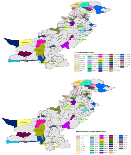
Figure 4. Theoretical vs. empirical distributions on several stations. The results of several stations are presented. However, the theoretical vs. empirical distributions on other stations can be observed accordingly.

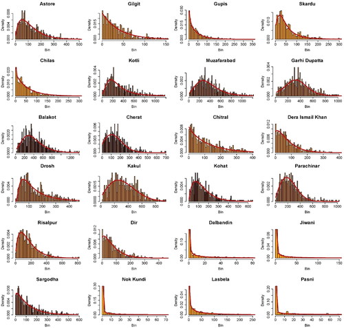
Figure 5. The temporal behaviour of SPI-3 on varying stations. The specific stations are presented, however, the temporal behaviour of SPI-3 other selected stations can be observed accordingly.

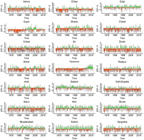
Figure 6. Temporal behaviour of SPI-3 ≤ 0 in various stations. The maximum and minimum drought for each year is provided. For instance, the maximum and minimum drought occurred in Astore is 12 and 5, respectively, from January 1971 to December 2017.

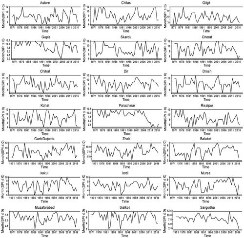
Table 1. Climatological characteristics of the precipitation are given for the various stations.

						1st		3rd
Variable	Stations	Latitude	Elevation (m)	longitude	Mean	Quartile	Median	Quartile	Kurtosis	St. Dev
Precipitation	Hyderabad	35.357	2546	74.8624	13.40	0.00	0.00	6.13	17.17	36.11
	Jacobabad	35.4206	1265	74.0967	11.35	0.00	0.30	6.10	96.64	38.52
	Nawabshah	35.9208	1500	74.3144	12.15	0.00	0.00	4.43	31.90	37.48
	Jiwani	36.2274	2206	73.4421	8.77	0.00	0.00	2.18	32.44	26.38
	Kalat	35.3247	2228	75.551	16.00	0.00	1.25	16.90	92.45	35.21
	Cherat	33.8215	892	71.8883	51.68	10.00	33.15	74.23	7.06	59.26
	Chitral	36	1494	72.12	37.44	3.73	20.15	58.33	3.28	44.38
	Dir	35.2074	1420	71.8768	116.43	46.00	98.00	173.43	2.08	90.33
	Drosh	35.5684	1359	71.8038	47.25	12.48	32.50	68.08	1.89	46.10
	Kohat	33.4	489	71.4414	47.74	11.95	30.60	66.00	11.49	55.84
	Parachinar	33.8992	1705	70.1008	82.56	30.53	63.75	112.50	4.32	74.22
	Risalpur	34.0751	309	71.9876	56.18	9.00	32.10	74.93	7.88	69.26
	Zhob	31.3417	1426	69.4486	23.68	2.00	13.15	31.68	3.90	29.34
	Balakot	34.5482	981	73.3532	132.68	46.90	101.10	187.18	5.76	121.10
	Garhi Dupatta	34.45	829	73.6157	122.14	46.93	97.70	171.68	1.66	100.04
	Kakul	34.15	1256	73.2167	111.44	39.38	85.60	162.25	1.07	93.17
	Kotli	33.5156	1735	73.9019	104.15	29.18	69.25	140.40	3.76	109.14
	Murree	33.907	2291	73.47	146.18	47.20	112.15	216.08	1.31	127.19
	Muzafarabad	34.25	737	73.62	124.37	43.65	97.20	176.03	4.97	113.12
	Sialkot	32.5	256	74.5333	84.04	9.08	37.30	93.08	10.97	128.98
	Sargodha	32.074	190	72.6861	40.05	4.00	20.25	50.58	6.29	55.61

The climatological features of precipitation are presented for the specific stations; however, the observed characteristics in other stations can be presented accordingly.

Table 2. The various probability distributions and their BIC are given.

Stations	Distribution	BIC	Stations	Distribution	BIC
Astore	Gamma	−1279.051	Dir	3P Weibull	−1504.677
Gupis	Gamma	−1264.948	Dalbandin	3P Weibull	−813.16
Gilgit	Exponential	−824.219	Jiwani	Generalized normal	−737.6675
Skardu	Generalized Extreme Value	−653.9913	Kalat	4P beta	−911.1111
Chilas	3P Weibull	−810.2973	Lasbela	4P beta	−1021.092
Kotli	Generalized Extreme Value	−1478.206	Nok Kundi	Generalized normal	−859.3224
Muzaffarabad	Gumbel	−1540.485	Panjgur	3P Weibull	−772.0721
Garhi Dupatta	Logistic	−1727.818	Pasni	3P Weibull	−1033.253
Balakot	Gumbel	−1777.455	Quetta	3P Weibull	−1369.229
Cherat	Rayleigh	−1620.881	Zhob	4P beta	−1281.465
Chitral	Gamma	−888.9078	Khuzdar	4P beta	−933.4191
D-I-Khan	3P Weibull	−1504.677	Badin	4P beta	−1218.033
Drosh	Log-Normal	−1049.803	Hyderabad	3P Weibull	−1042.638
Kakul	Rayleigh	−1170.1	Jacobabad	Generalized normal	−1319.438
Kohat	Gamma	−1481.598	Karachi airport	3P Weibull	−1067.376
Parachinar	Rayleigh	−1315.792	Nawabshah	4P Beta	−1550.361
Risalpur	Gamma	−1047.015	Faisalabad	3P Weibull	−1282.26
Khanpur	3P Weibull	−863.4623	Bahawalnagar	3P Weibull	−904.6014
Lahore	Log-Normal	−1320.925	Murree	Gumbel	−1614.46
Mianwali	Gamma	−947.6095	Sargodha	Gamma	−1347.796
Multan	Gamma	−964.9333	Sialkot	Johnson SU	−1179.503

These distributions are selected as appropriate for the standardization of the precipitation data at a three-month time scale.

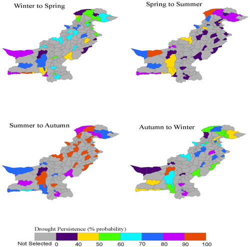
The average month of SPI ≤ 0 for selected stations across years can be observed in Figure 7. Figure 8 indicates the drought count in 47 years for the selected station. The annual drought average for Dir, Astore, Badin, Kalat, Bahawalnagar and Jacobabad are 8.2127, 8.1276, 7.1489, 5.8085, 5.3404 and 5.8723; similar behaviour can be observed in other stations. Further, the numerical quantification of drought frequency in a certain station can be achieved by dividing the total number of months with SPI ≤ 0, to the total number of months (from January 1971 to December 2017). In the current research, the data of each station are categorized into four seasons (Winter, Spring, Summer and Autumn). Therefore, knowledge regarding the seasonal drought frequency is important. Hence, seasonal drought frequency is calculated by the percentage of seasons in which drought SPI ≤ 0 occurs over the studied period for various seasons (autumn, winter, spring and summer). The varying behaviour of seasonal drought frequency is presented in Figure 9. Seasonal drought persistence is calculated as the total number of years in which drought continues from one season to the next divided by the total number of years in which SPI ≤ 0 in the preceding season. The probability of drought persistence is presented in Figure 10. It can be observed that the probability of drought persistence is high in Summer–Autumn.

Figure 7. The latitude and longitude of the selected stations and their monthly average drought for SPI-3 < 0 in selected time period.

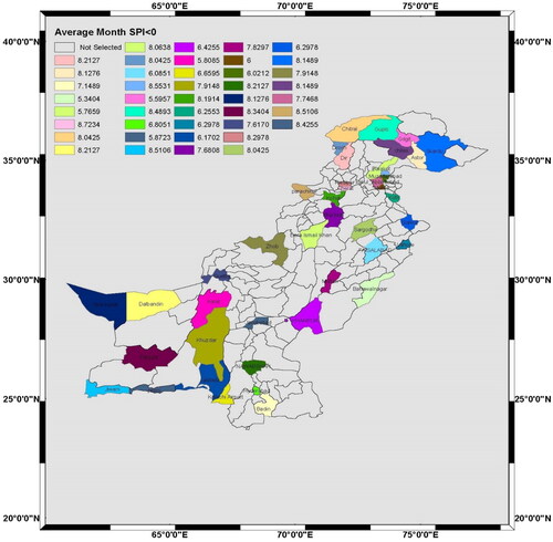
Figure 8. The total number of counts with SPI-3 ≤ 0 in the selected stations.

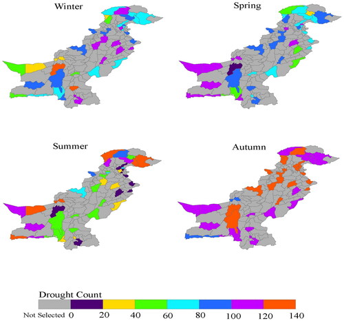
Figure 9. Seasonal drought frequency for each selected station.

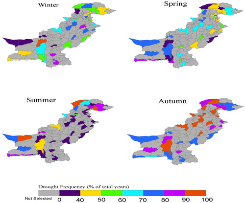
Figure 10. Drought Persistence percent probability for selected stations.

Table 3 presents information about the winter-spring drought persistence modelling. The log-likelihood values, WCT, LRCST and p values for the RELRM & CFELRM are given. The significant values of the tests of both models indicate that the RELRM & CFELRM are important. However, the HT is employed to substantiate the more suitable model for the current data set. The p value (0.6847) of the HT confirms that the RELRM is an appropriate choice for the spatiotemporal winter-spring drought persistence modelling. In Table 4, the results of the RELRM are given and interpreted accordingly. The coefficient of SPI with an odds ratio ($0.1624),$ indicates that an increment in the SPI-3 values in the winter season will decrease the probability of drought occurrences in spring.

Table 3. Information regarding the winter-spring drought persistence modelling is provided.

RELRM		CFELRM
Test	Values	Test	Values
Log likelihood	−2768.6023	Log likelihood	−2597.5633
Wald chi^2(1)	1110.32	LR chi^2(1)	1702.85
Prob > chi^2	0.0001	Prob > chi^2	0.0001

The log-likelihood values, WCT, LRCST and p values for the RELRM and CFELRM are given. The significant values of the tests of both models indicate that the RELRM and CFELRM are important.

Table 4. The results obtained from the RELRM are provided for the winter-to-spring meteorological drought persistence.

Coefficient RELRM
drought	Coefficient	Std. error	z	P>|z|	[95% conf.	interval]
SPI-3	−1.8177	0.0546	−33.32	0.0001	−1.9246	−1.7107
RELRM (odds ratio)
drought	Odds ratio	Std. error	z	P>|z|	[95% conf.	interval]
SPI-3	0.1624	0.0089	−33.32	0.0001	0.1459	0.1807
_cons	0.2624	0.0284	−12.35	0.0001	0.2122	0.3245
sigma_u	0.6453	0.0813			0.5041	0.8261
rho	0.1123	0.0251			0.0717	0.1718

The coefficient of SPI with odds ratio ($0.1624),$ shows that increment in the SPI-3 values in winter season will decline the probability of drought occurrences in spring. The $\rho =0.1124,$ shows the panel level of variation is almost 11% and the Likelihood Ratio test is significant which validates the effects of panel data modelling.

LR test of rho = 0 chibar2(01) = 262.10; Prob > = chibar2 = 0.0001.

Further, $\rho =\frac{{\delta }_{\mu }^2}{{\delta }_{\mu }^2+{\delta }_{\in }^2}$ is the proportion of variance explained by panel-level of variance component. where ${\delta }_{\mu }^2$ is the panel level of variance and ${\delta }_{\in }^2$ is the variation of the error term, $\in .$ The $\in$ is distributed with mean zero and variance $\frac{{\pi }^2}{3}.$ When $\rho$ is zero, it means no importance of the panel-level of variance component. In the current analysis, the $\rho =0.1124,$ showing the panel level of variation is almost 11%, and the Likelihood Ratio test is significant, which validates the effects of panel data modelling. Table 5 presents the results about the spring-summer spatiotemporal drought persistence modelling. The log-likelihood values, WCT, LRCST and p values for the RELRM & CFELRM are given. Based on HT with p value = 0.0009, it shows that the CFELRM is an appropriate choice for the spatiotemporal spring-to-summer drought persistence modelling. In Table 6, the results obtained from CFELRM are given. The significant coefficient of SPI-3 has an odd ratio $(0.1942)$ (95% confidence interval is −1.7754 to −1.5427), indicating that an increment in moisture conditions of the spring season will decrease the probability of the drought in the summer season. The odds ratio of 0.1942 means that there is a 19.42% chance of being in a higher category (i.e. 1 = drought). It means the most likely to stay in the lower category (i.e. 0 = No drought). Table 7 provides a description of the spatiotemporal drought persistence modelling in summer-to-autumn. The log-likelihood values, WCT, LRCST and p values for the RELRM & CFELRM are provided accordingly. Based HT with a p-value (0.541) substantiates the RELRM is an appropriate choice for the summer-to-autumn spatiotemporal drought persistence analysis. In Table 8, the coefficient of SPI-3 with an odd ratio (0.0673) indicates an increase in the SPI-3 values in the summer season; the drought will be less likely to occur in autumn. The likelihood ratio test for $\rho$ is significant, meaning the panel-level of variance component is almost 15%. Similarly, the log-likelihood values, WCT, LRCST and p values for the RELRM & CFELRM are provided in Table 9. The HT with a p-value (0.5683) suggests that the RELRM is more appropriate for the persistence of summer to autumn drought. The odds ratio (Table 10) of the SPI-3 is significant for the autumn-to-winter drought. The 95% confidence interval for the odds ratio of SPI-3 is −0.8481 to −0. 6938. The odd ratio shows that an increment in moisture conditions during the autumn season will decline the probability of drought in the winter season. Conclusively, the binary outcome panel data models provide comprehensive spatiotemporal information about the selected stations of Pakistan. Further, the results obtained from the current research would be considered for the current scenario and application site; however, they cannot be generalized for other climatic conditions. As climatology conditions of the selected region will change the outcomes and influence the extrapolations.

Table 5. The results about the spring-summer spatiotemporal drought persistence modelling.

RELRM		CFELRM
Test	values	Test	values
Log likelihood	−2062.6330	Log likelihood	−1880.6352
Wald chi2(1)	781.37	LR chi^2(1)	1159.00
Prob > chi^2	0.0001	Prob > chi^2	0.0001

The log-likelihood values, WCT, LRCST and p values for the RELRM and CFELRM are given.

Table 6. The results obtained from the CFELRM are given for the spring-to-summer meteorological drought persistence.

CFELRM
drought	Coefficient	Std. error	z	P>|z|	[95% conf.	interval]
SPI-3	−1.6387	0.0592	−27.66	0.0001	−1.7548	−1.5226
CFELRM
drought	Odds ratio	Std. error	z	P>|z|	[95% conf.	interval]
SPI-3	0.1942	0.0115	−27.66	0.0001	0.1729	0.2182

The significant coefficient of SPI-3 has the odd ratio $(0.1942)$ (95% confidence interval is −1.7754 to −1.5427) implying that an increment in moisture conditions of spring season will decline the probability of the drought in summer season. The odds ratio 0.1942 indicates that 19.42% chance of being in a higher category (i.e. 1= drought). It implies the most likely to stay in lower category (i.e. 0 = No drought).

Table 7. The log-likelihood values, LRCST and WCT for RELRM and CFELRM are computed for the summer-to-autumn meteorological drought persistence.

RELRM		CFELRM
Test	Values	Test	Values
Log likelihood	−1828.4793	Log likelihood	−1673.1925
Wald chi^2(1)	1169.78	LR chi^2(1)	2514.13
Prob > chi^2	0.0001	Prob > chi^2	0.0001

Table 8. The results found from the RELRM are provided for the summer-to-autumn meteorological drought persistence.

RELRM
drought	Coefficient	Std. error	z	P>|z|	[95% conf.	interval]
SPI-3	−2.6990	0.0789	−34.20	0.0001	−2.8537	−2.5443
RELRM
drought	Odds ratio	Std. error	z	P>|z|	[95% conf.	interval]
SPI-3	0.0673	0.0053	−34.20	0.0001	0.0576	0.0785
_cons	0.3899	0.0497	−7.39	0.0001	0.3037	0.5006
sigma_u	0.7584	0.0994			0.5865	0.9807
rho	0.1488	0.0332			0.0947	0.2262

LR test of rho = 0 chibar2(01) = 208.07; Prob > = chibar2 = 0.0001.

Table 9. The values obtained from the various tests for RELRM and CFELRM are given for the autumn-to-winter meteorological drought persistence.

RELRM		CFELRM
Test	Values	Test	Values
Log likelihood	−3556.6109	Log likelihood	−3368.0259
Wald chi2(1)	383.4	LR chi2(1)	422.50
Prob > chi2	0.0001	Prob > chi2	0.0001

Table 10. The results attained from the RELRM are provided for the autumn-to-winter meteorological drought persistence.

RELRM
drought	Coefficient	Std. error	Z	P>|z|	[95% conf.	interval]
SPI-3	−0.7709	0.0394	−19.58	0.0001	−0.8481	−0.6938
RELRM
drought	Odds ratio	Std. error	z	P>|z|	[95% conf.	interval]
SPI-3	0.4626	0.0182	−19.58	0.0001	0.4282	0.4997
_cons	0.4740	0.0593	−5.97	0.0001	0.3709	0.6057
sigma_u	0.7385	0.0874			0.5856	0.9313
rho	0.1422	0.0289			0.0944	0.2086

The 95% confidence interval for the odds ratio of SPI-3 is −0.8481 to −0. 6938. The odd ratio indicates that an increment in moisture conditions during the autumn season will decrease the probability of drought in the winter season. The significant value of $\rho (0.1422)$ is the panel level of variance which shows 14.22% of the total variance.

LR test of rho = 0 chibar2(01) = 502.35; Prob > = chibar2 = 0.000.

4. Discussion

Early warning and monitoring are critical elements of drought preparedness and mitigation plans. Several studies have developed techniques to monitor and predict drought occurrences in different climatic conditions (Nayak and Hassan 2021; Alawsi et al. 2022; Cerpa Reyes et al. 2022; Dikshit et al. 2022; Kamali and Asghari 2022; Elbeltagi et al. 2023;). Linear regression is utilized frequently in literature for statistical prediction (Güner Bacanli 2017; Kim et al. 2020; Papadopoulos et al. 2021). Generally, these regression models mainly deal with the continuous case of the dependent variable. The linear regression models cannot work properly for the categorical response variable. Thus, categorically based modelling is generally established, for instance, logistic regression, multiple logistic regression, ordered logistic regression, etc. (Ford and Labosier 2014; Bachmair et al. 2017; Meng et al. 2017; Seo et al; Niaz, Zhang, et al. 2021; Niaz, Raza, et al. 2022). Ford and Labosier (2014) have employed logistic regression to examine drought persistence in different stations. Meng et al. (2017) utilized logistic regression to investigate the spatial pattern of drought. Kuwayama et al. (2019) used panel data models with fixed effects that exploited spatial and temporal variations in drought conditions. Sun et al. (2019) used panel data models for identifying key factors of affecting regional drought. The study found that the use of panel data model had objectively and comprehensively reflected the actual situation of the drought in the region. Moreover, Defrance et al. (2020) used panel data model to address spatial impact of drought. Although the mentioned studies have identified the greater detail about drought occurrences and their impacts based on several variables. However, the identification of the inter-seasonal drought characteristics is important. For this purpose, recently, Niaz, Raza, et al. (2022) applied a proportional odds model to identify inter-seasonal drought characteristics in various stations. However, these findings have not focused on the spatiotemporal effect of meteorological drought. This study is mainly focused on spatiotemporal and inter-seasonal drought characteristics. The SPI at a 3-month time scale is utilized to identify the drought characteristics in various seasons. The binary outcome panel data models containing RELRM and CFELRM are employed for finding the spatiotemporal and inter-seasonal drought persistence in certain stations. The LRCST and WCT test are used to measure the significance of RELRM and CFELRM. The LRCST and WCT are significant for RELRM and CFELRM. Hence the LRCST and WCT substantiate that the use of RELRM and CFELRM is vital for the current analysis. However, based on HT, the selected model is utilized for identifying the spatiotemporal and inter-seasonal drought persistence in certain stations accordingly. Further, in the literature, none of the authors have considered the binary outcome panel data models for the meteorological drought analysis, specifically for seasonal drought analysis. Thus, the spatiotemporal study of drought occurrences based on binary outcome panel data model is an innovative step in the literature that may help meteorologists and scientific researchers to substantiate their modelling. Moreover, the outcomes of the current analysis provide the groundwork for paying more attention to early warning systems for effectively managing water resources to avoid negative drought impacts in Pakistan. In addition, these models can be more effective for other drought indices that incorporate more climate variables.

5. Conclusion

Knowledge of spatiotemporal and inter-seasonal drought characteristics can obliquely support diminishing the potential negative influences of drought. The binary outcome panel data models including RELRM and CFELRM are utilized to find the spatiotemporal and inter-seasonal drought persistence in selected stations. The LRCST and WCT test are used to measure the significance of RELRM and CFELRM. The log-likelihood values, WCT, LRCST and p values for the RELRM and CFELRM are calculated for the drought persistence modelling in various seasons. For instance, in the winter-spring drought persistence modelling the significant values of the tests of both models indicate their importance for the winter-spring drought persistence modelling. However, the HT is employed to substantiate the more suitable model for the current data set. The p value (0.6847) of the HT confirms that the RELRM is an appropriate choice for the spatiotemporal winter-spring drought persistence modelling. The coefficient of SPI with an odd ratio ($0.1624$) indicates that increasing the SPI-3 values in winter will decrease the probability of drought occurrences in spring. The $\rho =0.1124,$ shows the panel level of variation is almost 11%, and the Likelihood Ratio test is significant which validates the effects of panel data modeling. Further, the CFELRM is an appropriate choice for the spatiotemporal spring to summer drought persistence modelling. The significant coefficient of SPI-3 with an odd ratio of $0.1942$ (95% confidence interval is −1.7754 to −1.5427) indicates that an increment in moisture conditions during the spring season will reduce the probability of drought in the summer season. The odds ratio 0.1942 means that 19.42% chances of being in higher category (i.e. 1= drought). It means the most likely to stay in the lower category (i.e. 0 = No drought). Based HT with a p value (0.541) substantiates the RELRM is an appropriate choice for the summer-to-autumn spatiotemporal drought persistence analysis. Similarly, the RELRM is selected for the summer-to-autumn and autumn-to-winter spatiotemporal drought persistence analysis. Conclusively, the binary outcome panel data models provide comprehensive spatiotemporal information about the selected stations of Pakistan. The outcomes of the current analysis contributes to a growing literature and can serve as an early warning to the effective management of water resources to avoid the negative drought impacts in Pakistan.

Ethical statement

All procedures followed were in accordance with the ethical standards of the Helsinki Declaration of 1975, as revised in 2000.

Consent to participate

All authors voluntarily agreed to participate in this research study.

Acknowledgements

The authors extend Their appreciation to the Deanship of Scientific Research at King Khalid University for funding this work through Larg Groups. (Project under grant number (RGP.2/4/43). And this study is supported via funding from Prince Sattam bin Abdulaziz University project number (PSAU/2023/R/1444).

Availability of data and codes

The data and codes used for the preparation of the manuscript are available with the corresponding author and can be provided upon request.

Disclosure statement

The authors declare that they have no known competing financial interests or personal relationships that could have influenced the work reported in this article.

References

- Adib A, Marashi SS. 2019. Meteorological drought monitoring and preparation of long-term and short-term drought zoning maps using regional frequency analysis and L-moment in the Khuzestan province of Iran. Theor Appl Climatol. 137(1–2):77–87.
- Adib A, Tavancheh F. 2019. Relationship between hydrologic and metrological droughts using the streamflow drought indices and standardized precipitation indices in the Dez Watershed of Iran. Int J Civ Eng. 17(7):1171–1181.
- Ali Z, Hussain I, Faisal M, Khan DM, Niaz R, Elashkar EE, Shoukry AM. 2020. Propagation of the multi-scalar aggregative standardized precipitation temperature index and its application. Water Resour Manage. 34(2):699–714.
- Ali Z, Hussain I, Faisal M, Nazir HM, Moemen MAE, Hussain T, Shamsuddin S. 2017. A novel multi-scalar drought index for monitoring drought: the standardized precipitation temperature index. Water Resour Manage. 31(15):4957–4969.
- Aadhar S, Mishra V. 2022. Challenges in drought monitoring and assessment in India. Water Secur. 16:100120.
- Afshar MH, Bulut B, Duzenli E, Amjad M, Yilmaz MT. 2022. Global spatiotemporal consistency between meteorological and soil moisture drought indices. Agric For Meteorol. 316:108848.
- Alahacoon N, Edirisinghe M. 2022. A comprehensive assessment of remote sensing and traditional based drought monitoring indices at global and regional scale. Geomatics Nat Hazards Risk. 13(1):762–799.
- Alawsi MA, Zubaidi SL, Al-Bdairi NSS, Al-Ansari N, Hashim K. 2022. Drought forecasting: a review and assessment of the hybrid techniques and data pre-processing. Hydrology. 9(7):115.
- Anderegg WR, Trugman AT, Badgley G, Konings AG, Shaw J. 2020. Divergent forest sensitivity to repeated extreme droughts. Nat Clim Chang. 10(12):1091–1095.
- Angelidis P, Maris F, Kotsovinos N, Hrissanthou V. 2012. Computation of drought index SPI with alternative distribution functions. Water Resour Manage. 26(9):2453–2473.
- Anjum SA, Saleem MF, Cheema MA, Bilal MF, Khaliq T. 2012. An assessment to vulnerability, extent, characteristics and severity of drought hazard in Pakistan. Pak J Sci. 64(2):138.
- Arabameri A, Chandra Pal S, Santosh M, Chakrabortty R, Roy P, Moayedi H. 2022. Drought risk assessment: integrating meteorological, hydrological, agricultural and socio-economic factors using ensemble models and geospatial techniques. Geocarto Int. 37(21):6087–6115.
- Arellano M, Carrasco R. 2003. Binary choice panel data models with predetermined variables. J Econometr. 115(1):125–157.
- Aryal Y, Zhu J. 2021. Evaluating the performance of regional climate models to simulate the US drought and its connection with El Nino Southern Oscillation. Theor Appl Climatol. 145(3–4):1259–1273.
- Bachmair S, Svensson C, Prosdocimi I, Hannaford J, Stahl K. 2017. Developing drought impact functions for drought risk management. Nat Hazards Earth Syst Sci. 17(11):1947–1960.
- Bae H, Ji H, Lim YJ, Ryu Y, Kim MH, Kim BJ. 2019. Characteristics of drought propagation in South Korea: relationship between meteorological, agricultural, and hydrological droughts. Nat Hazards. 99(1):1–16.
- Cerpa Reyes LJ, Ávila Rangel H, Herazo LCS. 2022. Adjustment of the standardized precipitation index (SPI) for the evaluation of drought in the arroyo pechelín basin, Colombia, under zero monthly precipitation conditions. Atmosphere. 13(2):236.
- Charbonneau KB. 2017. Multiple fixed effects in binary response panel data models. Econometr J. 20(3):S1–S13.
- Chauhan V, Suman HK, Bolia NB. 2016. Binary logistic model for estimation of mode shift into Delhi Metro. Open Trans J. 10(1):124–136.
- Chen XD, Su Y, Fang XQ. 2021. Social impacts of extreme drought event in Guanzhong area, Shaanxi Province, during 1928–1931. Clim Change. 164(3–4):1–19.
- Cunha APMA, Zeri M, Deusdará Leal K, Costa L, Cuartas LA, Marengo JA, Tomasella J, Vieira RM, Barbosa AA, Cunningham C, et al. 2019. Extreme drought events over Brazil from 2011 to 2019. Atmosphere. 10(11):642.
- Defrance D, Delesalle E, Gubert F. 2020. Is migration drought-induced in Mali? An empirical analysis using panel data on Malian localities over the 1987–2009 period (No. UCL-Université Catholique de Louvain). Louvain-la-Neuve, Belgium: Institut de Recherche Economiques et Sociales, UC Louvain.
- Deng L, Peng C, Kim D-G, Li J, Liu Y, Hai X, Liu Q, Huang C, Shangguan Z, Kuzyakov Y. 2021. Drought effects on soil carbon and nitrogen dynamics in global natural ecosystems. Earth Sci Rev. 214:103501.
- Dikshit A, Pradhan B, Santosh M. 2022. Artificial neural networks in drought prediction in the 21st century–A scientometric analysis. Appl Soft Comput. 114:108080.
- Ding Y, Xu J, Wang X, Cai H, Zhou Z, Sun Y, Shi H. 2021. Propagation of meteorological to hydrological drought for different climate regions in China. J Environ Manage. 283:111980.
- Elbeltagi A, Kumar M, Kushwaha NL, Pande CB, Ditthakit P, Vishwakarma DK, Subeesh A. 2023. Drought indicator analysis and forecasting using data driven models: case study in Jaisalmer, India. Stoch Environ Res Risk Assess. 37(1):113–131.
- Esfahanian E, Nejadhashemi AP, Abouali M, Adhikari U, Zhang Z, Daneshvar F, Herman MR. 2017. Development and evaluation of a comprehensive drought index. J Environ Manage. 185:31–43.
- Farahmand A, AghaKouchak A. 2015. A generalized framework for deriving nonparametric standardized drought indicators. Adv Water Resour. 76:140–145.
- Ford T, Labosier CF. 2014. Spatial patterns of drought persistence in the Southeastern United States. Int J Climatol. 34(7):2229–2240.
- Güner Bacanli Ü. 2017. Trend analysis of precipitation and drought in the Aegean region, Turkey. Met Apps. 24(2):239–249.
- Guo Y, Huang S, Huang Q, Leng G, Fang W, Wang L, Wang H. 2020. Propagation thresholds of meteorological drought for triggering hydrological drought at various levels. Sci Total Environ. 712:136502.
- Ha TV, Huth J, Bachofer F, Kuenzer C. 2022. A review of earth observation-based drought studies in Southeast Asia. Remote Sensing. 14(15):3763.
- Haile GG, Tang Q, Li W, Liu X, Zhang X. 2020. Drought: progress in broadening its understanding. Wiley Interdiscip Rev: water. 7(2):e1407.
- Han J, Yang Y. 2021. The socio-economic effects of extreme drought events in northern China on the Ming dynasty in the late fifteenth century. Clim Change. 164(3–4):1–17.
- Haroon MA, Zhang J, Yao F. 2016. Drought monitoring and performance evaluation of MODIS-based drought severity index (DSI) over Pakistan. Nat Hazards. 84(2):1349–1366.
- Hassan AG, Fullen MA, Oloke D. 2019. Problems of drought and its management in Yobe State, Nigeria. Weather Clim Extremes. 23:100192.
- Honoré BE, Lewbel A. 2002. Semiparametric binary choice panel data models without strictly exogeneous regressors. Econometrica. 70(5):2053–2063.
- Horowitz JL, Savin NE. 2001. Binary response models: logits, probits and semiparametrics. Journal of Economic Perspectives. 15(4):43–56.
- Hussain A, Jadoon KZ, Rahman KU, Shang S, Shahid M, Ejaz N, Khan H. 2023. Analyzing the impact of drought on agriculture: evidence from Pakistan using standardized precipitation evapotranspiration index. Nat Hazards. 115(1):389–408.
- Idrees M, Shahzad N, Afzal F. 2022. Growing climate change impacts on hydrological drought and food security in district Peshawar, Pakistan. Handbook of climate change across the food supply chain. Cham, Switzerland: Springer; p. 467–483.
- Jordaan A. 2022. Drought: the case of South Africa. Routledge handbook of environmental hazards and society. Abingdon: Routledge; p. 106–124
- Kamali S, Asghari K. 2022. The effect of meteorological and hydrological drought on groundwater storage under climate change scenarios. Water Resour Manage. 1–19.
- Kao SC, Govindaraju RS. 2010. A copula-based joint deficit index for droughts. J Hydrol. 380(1–2):121–134.
- Keyantash JA, Dracup JA. 2004. An aggregate drought index: assessing drought severity based on fluctuations in the hydrologic cycle and surface water storage. Water Resour Res. 40(9)
- Kim SW, Jung D, Choung YJ. 2020. Development of a multiple linear regression model for meteorological drought index estimation based on landsat satellite imagery. Water. 12(12):3393.
- Kim TW, Jehanzaib M. 2020. Drought risk analysis, forecasting and assessment under climate change. Water. 12(7):1862.
- Kleinbaum DG, Klein M. 2010. Assessing discriminatory performance of a binary logistic model: ROC curves. Logistic regression. New York (NY): Springer; p. 345–387.
- Kuwayama Y, Thompson A, Bernknopf R, Zaitchik B, Vail P. 2019. Estimating the impact of drought on agriculture using the US Drought Monitor. Am J Agric Econ. 101(1):193–210.
- Lee BR, Sung JH, Chung ES, Ministry of Public Safety and Security, National Disaster Management Institute, Disaster Information Research Division. 2015. Comparison of meteorological drought and hydrological drought index. J. Korea Water Resour. Assoc. 48(1):69–78.
- Li X, He B, Quan X, Liao Z, Bai X 2015. Use of the standardized precipitation evapotranspiration index (SPEI) to characterize the drying trend in southwest China from 1982–2012. Remote Sens. 7(8):10917–10937.
- Li L, She D, Zheng H, Lin P, Yang ZL. 2020. Elucidating diverse drought characteristics from two meteorological drought indices (SPI and SPEI) in China. J Hydrometeorol. 21(7):1513–1530.
- Lotfirad M, Esmaeili-Gisavandani H, Adib A. 2022. Drought monitoring and prediction using SPI, SPEI, and random forest model in various climates of Iran. J Water Clim Change. 13(2):383–406.
- Manski CF. 1988. Identification of binary response models. J Am Stat Assoc. 83(403):729–738.
- Masanta SK, Srinivas VV. 2022. Proposal and evaluation of nonstationary versions of SPEI and SDDI based on climate covariates for regional drought analysis. J Hydrol. 610:127808.
- McKee TB, Doesken NJ, Kleist J. 1993. The relationship of drought frequency and duration to time scales. Proceedings of the 8th conference on applied climatology. Vol. 17. Boston (MA): American Meteorological Society; p. 179–183.
- Meng L, Ford T, Guo Y. 2017. Logistic regression analysis of drought persistence in East China. Int J Climatol. 37(3):1444–1455.
- Mishra AK, Singh VP. 2010. A review of drought concepts. J Hydrol. 391(1–2):202–216.
- Mishra AK, Singh VP. 2011. Drought modeling–A review. J Hydrol. 403(1–2):157–175.
- Mokhtar A, Jalali M, He H, Al-Ansari N, Elbeltagi A, Alsafadi K, Abdo HG, Sammen SS, Gyasi-Agyei Y, Rodrigo-Comino J. 2021. Estimation of SPEI meteorological drought using machine learning algorithms. IEEE Access. 9:65503–65523.
- Mondol MAH, Zhu X, Dunkerley D, Henley BJ. 2021. Observed meteorological drought trends in Bangladesh identified with the Effective Drought Index (EDI). Agric Water Manage. 255:107001.
- Niaz R, Raza MA, Almazah MM, Hussain I, Al-Rezami AY, Al-Shamiri MMA. 2022. Proportional odds model for identifying spatial inter-seasonal propagation of meteorological drought. Geomatics Nat Hazards Risk. 13(1):1614–1639.
- Niaz R, Iqbal N, Al-Ansari N, Hussain I, Elsherbini Elashkar E, Shamshoddin Soudagar S, Gani SH, Mohamd Shoukry A, Sh. Sammen S. 2022. A new spatiotemporal two-stage standardized weighted procedure for regional drought analysis. PeerJ. 10:e13249.
- Niaz R, Tanveer F, Almazah M, Hussain I, Alkhatib S, Al-Razami AY. 2022. Characterization of meteorological drought using Monte Carlo feature selection and steady-state probabilities. Complexity. 2022:1–19.
- Niaz R, Almazah MM, Al-Duais FS, Iqbal N, Khan DM, Hussain I. 2022. Spatiotemporal analysis of meteorological drought variability in a homogeneous region using standardized drought indices. Geomatics Nat Hazards Risk. 13(1):1457–1481.
- Niaz R, Almazah MM, Hussain I, Faisal M, Al-Rezami AY, Naser MA. 2022. A new comprehensive approach for regional drought monitoring. PeerJ. 10:e13377.
- Niaz R, Almazah MMA, Hussain I, Filho JDP, Al-Ansari N, Sh Sammen S. 2022. Assessing the probability of drought severity in a homogenous region. Complexity. 2022:1–8.
- Niaz R, Zhang X, Ali Z, Hussain I, Faisal M, Elashkar EE, Khader JA, Soudagar SS, Shoukry AM, Al-Deek FF. 2021. A new propagation-based framework to enhance competency in regional drought monitoring. Tellus A Dynm Meteorol Oceanogr. 73(1):1975404–1975412.
- Niaz R, Hussain I, Zhang X, Ali Z, Elashkar EE, Khader JA, Soudagar SS, Shoukry AM. 2021. Prediction of drought severity using model-based clustering. Math Prob Eng. 2021:1–10.
- Niaz R, Hussain I, Ali Z, Faisal M. 2021. A novel framework for regional pattern recognition of drought intensities. Arab J Geosci. 14(16):1–16.
- Niaz R, Zhang X, Iqbal N, Almazah M, Hussain T, Hussain I. 2021. Logistic regression analysis for spatial patterns of drought persistence. Complexity. 2021:1–13.
- Niaz R, Almazah M, Zhang X, Hussain I, Faisal M. 2021. Prediction for various drought classes using spatiotemporal categorical sequences. Complexity. 2021:1–11.
- Niaz R, Almazah MMA, Hussain I, Filho JDP. 2021. A new framework to substantiate the prevalence of drought intensities. Theor Appl Climatol. 147(3–4):1079–1090.
- Naresh Kumar M, Murthy CS, Sesha Sai MVR, Roy PS. 2009. On the use of Standardized Precipitation Index (SPI) for drought intensity assessment. Met Apps. 16(3):381–389.
- Nayak MA, Hassan WU. 2021. A synthesis of drought prediction research over India. Water Secur. 13:100092.
- Orimoloye IR, Belle JA, Orimoloye YM, Olusola AO, Ololade OO. 2022. Drought: a common environmental disaster. Atmosphere. 13(1):111.
- Palmer WC. 1965. Meteorological drought. Vol. 30. Bohemia (NY): US Department of Commerce, Weather Bureau.
- Papadopoulos C, Spiliotis M, Gkiougkis I, Pliakas F, Papadopoulos B. 2021. Fuzzy linear regression analysis for groundwater response to meteorological drought in the aquifer system of Xanthi plain, NE Greece. J Hydroinform. 23(5):1112–1129.
- Prodhan FA, Zhang J, Hasan SS, Sharma TPP, Mohana HP. 2022. A review of machine learning methods for drought hazard monitoring and forecasting: current research trends, challenges, and future research directions. Environ Modell Softw. 149:105327.
- Quiring SM. 2009. Monitoring drought: an evaluation of meteorological drought indices. Geography Compass. 3(1):64–88.
- Salimi H, Asadi E, Darbandi S. 2021. Meteorological and hydrological drought monitoring using several drought indices. Appl Water Sci. 11(2):1–10.
- Sánchez-Pinillos M, D’Orangeville L, Boulanger Y, Comeau P, Wang J, Taylor AR, Kneeshaw D. 2022. Sequential droughts: a silent trigger of boreal forest mortality. Glob Chang Biol. 28(2):542–556.
- Satoh Y, Shiogama H, Hanasaki N, Pokhrel Y, Boulange JES, Burek P, Gosling SN, Grillakis M, Koutroulis A, Müller Schmied H, et al. 2021. A quantitative evaluation of the issue of drought definition: a source of disagreement in future drought assessments. Environ Res Lett. 16(10):104001.
- Savelli E, Rusca M, Cloke H, Di Baldassarre G. 2022. Drought and society: scientific progress, blind spots, and future prospects. Wiley Interdiscip Rev Clim Change. 13:e761.
- Semykina A, Wooldridge JM. 2018. Binary response panel data models with sample selection and self‐selection. J Appl Econ. 33(2):179–197.
- Sharma A, Sen S. 2022. Droughts risk management strategies and determinants of preparedness: insights from Madhya Pradesh, India. Nat Hazards. 114(2):2243–2281.
- Solh M, van Ginkel M. 2014. Drought preparedness and drought mitigation in the developing world’s drylands. Weather Clim Extremes. 3:62–66.
- Spinoni J, Barbosa P, De Jager A, McCormick N, Naumann G, Vogt JV, Magni D, Masante D, Mazzeschi M. 2019. A new global database of meteorological drought events from 1951 to 2016. J Hydrol Reg Stud. 22:100593.
- Stagge JH, Tallaksen LM, Gudmundsson L, Van Loon AF, Stahl K. 2015. Candidate distributions for climatological drought indices (SPI and SPEI). Int J Climatol. 35(13):4027–4040.
- Sueyoshi GT. 1995. A class of binary response models for grouped duration data. J Appl Econ. 10(4):411–431.
- Sun H, Dang Y, Mao W. 2019. Identifying key factors of regional agricultural drought vulnerability using a panel data grey combined method. Nat Hazards. 98(2):621–642.
- Surendran U, Kumar V, Ramasubramoniam S, Raja P. 2017. Development of drought indices for semi-arid region using drought indices calculator (DrinC)–a case study from Madurai District, a semi-arid region in India. Water Resour Manage. 31(11):3593–3605.
- Sutradhar BC, Rao RP, Pandit VN. 2008. Generalized method of moments versus generalized quasilikelihood inferences in binary panel data models. Sankhyā Indian J Stat B (2008-). 70:34–62.
- Svoboda M, LeComte D, Hayes M, Heim R, Gleason K, Angel J, Rippey B, Tinker R, Palecki M, Stooksbury D, et al. 2002. The drought monitor. Bull Amer Meteor Soc. 83(8):1181–1190.
- Tareke KA, Awoke AG. 2022. Hydrological drought analysis using streamflow drought index (SDI) in Ethiopia. Adv Meteorol. 2022:1–19.
- Türkeş M, Tatlı H. 2009. Use of the standardized precipitation index (SPI) and a modified SPI for shaping the drought probabilities over Turkey. Int J Climatol A J Royal Meteorol Soc. 29(15):2270–2282.
- Vicente-Serrano SM, Beguería S, López-Moreno JI. 2010. A multiscalar drought index sensitive to global warming: the standardized precipitation evapotranspiration index. J Clim. 23(7):1696–1718.
- Vicente-Serrano SM, Peña-Angulo D, Beguería S, Domínguez-Castro F, Tomás-Burguera M, Noguera I, Gimeno-Sotelo L, El Kenawy A. 2022. Global drought trends and future projections. Philos Trans A Math Phys Eng Sci. 380(2238):20210285.
- Vogt, J. V., & Somma, F. (Eds.). 2013. Drought and drought mitigation in Europe. Vol. 14. Berlin, Germany: Springer Science & Business Media.
- Waseem M, Jaffry AH, Azam M, Ahmad I, Abbas A, Lee JE. 2022. Spatiotemporal Analysis of Drought and Agriculture Standardized Residual Yield Series Nexuses across Punjab, Pakistan. Water. 14(3):496.
- Waseem M, Khurshid T, Abbas A, Ahmad I, Javed Z. 2022. Impact of meteorological drought on agriculture production at different scales in Punjab, Pakistan. J Water Clim Change. 13(1):113–124.
- Yang J, Chang J, Wang Y, Li Y, Hu H, Chen Y, Huang Q, Yao J. 2018. Comprehensive drought characteristics analysis based on a nonlinear multivariate drought index. J Hydrol. 557:651–667.
- Yao Y, Fu B, Liu Y, Li Y, Wang S, Zhan T, Wang Y, Gao D. 2022. Evaluation of ecosystem resilience to drought based on drought intensity and recovery time. Agric for Meteorol. 314:108809.
- Yihdego Y, Vaheddoost B, Al-Weshah RA. 2019. Drought indices and indicators revisited. Arab J Geosci. 12(3):1–12.
- Zarei AR, Mahmoudi MR, Moghimi MM. 2023. Determining the most appropriate drought index using the random forest algorithm with an emphasis on agricultural drought. Nat Hazards. 115(1):923–946.
- Zarei AR, Mahmoudi MR. 2020. Assessment of the effect of PET calculation method on the Standardized Precipitation Evapotranspiration Index (SPEI). Arab J Geosci. 13(4):1–14.
- ZargaR A, Sadiq R, Naser B, Khan FI. 2011. A review of drought indices. Environ Rev. 19(NA):333–349.
- Zhao H, Gao G, An W, Zou X, Li H, Hou M. 2017. Timescale differences between SC-PDSI and SPEI for drought monitoring in China. Phys Chem Earth Parts a/b/c. 102:48–58.