Comparison of a Sentinel-2 land cover map obtained through multi-temporal analysis with the official forest cartography. the case of Galicia (Spain)

Abstract

In numerous countries, official forest cartography is obtained through photointerpretation of aerial images which hinders having up-to-date information. This study explores the usefulness of a land cover map produced automatically using Sentinel-2 images as a complement of the official Spanish forest map in Galicia. It was obtained a map with an Overall Accuracy of 86%. Both maps were compared. Net area covered by each forest class differed among maps, the differences were higher in areas managed with shorter rotation cycles. Main differences were due to the capabilities of Sentinel-2 to identify harvestings or disturbances and to the minimum mapping units of each map. The Sentinel-2 map had a higher ability to map trees outside the forest, and the official cartography hides small parcels and incipient land change dynamics. Sentinel-2 based maps could be a powerful tool to reduce the information gap considering the official cartography updating frames.

Keywords:

• Forest management
• remote sensing
• map
• satellite images

1. Introduction

Forestry resource mapping and quantification are key for forest stakeholders when it comes to the design, implementation and tracking of sustainable management measures (FAO, 2020). They are also essential for evaluating the impact of climate change, natural disasters, and biodiversity conservation initiatives as well as for quantifying carbon reservoirs (FAO, 2017). Geospatial forestry information is needed at differing scales (e.g. at the global, national, regional and local level), with varying levels of detail, and legend detail, and differing frequencies of update (Szantoi et al. 2021, Szantoi et al. 2020). The specifications needed depend on the extension of the area in question, the types of forest species of interest and the singularities of the forest sector under consideration.

In numerous countries, forest land cover maps are obtained through photointerpretation of aerial images and field surveys (Barrett et al. 2016). These kinds of methodologies allow for legends with a great degree of detail. However, they are quite time consuming and expensive. Consequently, maps are difficult to update (Costa et al. 2020, Gomez et al. 2019) and their feasibility for large areas may be limited. Despite Spain’s being one of the largest countries in the European Union, the official forest cartography, called the Spanish Forest Map (the MFE for its initials in Spanish), is generated using these kinds of procedures (MITERD 2011). The MFE describes the forest cover at the national level. Given the limitations of the methodology used to produce this cartography, its updating frame is low. The latest available map in 2023 was released in 2011 (MITERD 2011).

These photointerpretation-derived maps may be less useful for forestry stakeholders in regions characterized by having an active forestry sector, an abundance of fast-growing tree species, a high rate of land use changes or highly fragmented stands (Xunta de Galicia 2021, Gomez et al. 2019). In Galicia, a region in the Northwest of Spain, all of these circumstances apply, in cases even simultaneously (Spanish Government 2011; Levers et al. 2014; MITERD, 2018). The design of the MFE, with large minimum mapping units and a low frequency of update, means that sets of pure stands in neighboring small parcels in Galicia are grouped into large polygons and listed as mixed stands. Furthermore, the high rate of land use changes causes the MFE to rapidly become outdated in this region.

The latest advances in open-access satellite multispectral imagery, computing capabilities and image analysis techniques, provide the capability to automate forest mapping processes (Wulder et al. 2018) thus permitting the creation of thematic cartography at fine resolutions as well as increasing update frequency and reducing production time and overall cost. Some agencies are making advances in this field. The European Commission has developed the Forestry Information System for Europe (FISE), a site that compiles forestry data and thematic maps derived from the Copernicus Land Monitoring Program and other data sources such as the Member States’ NFIs. It has been specifically designed to support forestry-related decisions and policies at the EU level (FISE 2022). Another example of the shifting trend to remote sensing based cartography is Malinowski et al. (2020), they have developed a methodology that allows to automatically obtain Land Cover Maps of Europe using Sentinel-2 imagery that may substitute the previous existing similar product CORINE Land Cover whose production heavily relies on manual work (Büttner et al. 2017). This global maps are usually available at a 10 m or coarser spatial resolution, although the map legends are quite broad (forest and non-forest areas, percentage of forest cover, coniferous-broadleaf covers, etc.). Since maps should be adapted to user’s specific needs (Szantoi et al. 2021, Szantoi et al. 2020) national and regional maps have been developed using remote sensing as well. Therefore some countries have successfully implemented satellite-based methods in their NFIs to obtain forest resources distribution information adapted to their specific needs. This is the case of Finland and the USA (Barrett et al. 2016). Also there is the example Inglada et al. 2017 who have developed a methodology to produce land cover maps with detailed forest information at national scales or Nomura and Mitchard (2018) which have used Sentinel-2 images to locate Small plantations within complex forest landscapes. Also it is remarkable the work done by Ganz et al. to develop a Sentinel-2 forest cover map that have been proven to extent the information provided by the NFI in a German region within inventory cycles. In the specific case of Galicia, Alonso et al. (2021) recently proposed an optimized methodology to obtain forestry-oriented land cover maps that cover the information needs of this specific region using satellite imagery.

Considering these advances, satellite images can potentially be used as a complement to the official cartographic data sources. Several studies have indicated that open-access satellite images, such as those provided by Sentinel-2, provide useful geospatial forest information that can be updated annually and complement NFI data (Lang et al. 2018, Gomez et al. 2019, Ganz et al. 2020). Gomez et al. (2019)highlight the limitations of the MFE for forest predictions in Spain and show a wide range of opportunities that satellite imagery could offer to complement the information that the MFE provides.

This study generates an annual forest land cover map through a multitemporal approach based on Sentinel-2 data and the random forest algorithm (Alonso et al. 2021). The annual map of a region in the Northwest of Spain is obtained. This region is characterized by an active forestry sector, fast growing species and a great degree of stand fragmentation. The results are compared with the official Spanish forest cartography using two different approaches: net balance and spatial comparison. To this end, a procedure is designed to harmonize land cover legends and formats. The quantitative and qualitative results are analyzed in detail.

By doing this, this study aims to analyze the strengths and limitations of vector-based maps produced through high resolution imagery photointerpretation and field work, and pixel based maps obtained by supervised classification of medium resolution multispectral images in a region with an active forest sector, fast growing species and high stand fragmentation. Also, it aims to explore if a land cover map produced automatically using satellite imagery could help to update and improve the forest information provided by the Spanish forest official cartography in areas with those forest characteristics.

2. Study area

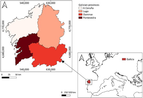
This study was conducted in Galicia, a region in the Northwest of Spain (see Figure 1) with an area of 29,589 square kilometers. In administrative terms, Galicia is divided into 4 provinces: A Coruña, Lugo, Ourense and Pontevedra (see Figure 1). According to the Köppen-Geiger classification Galicia has two types of climates Mediterranean-Oceanica, climate (Csb) on the coastal areas and Mediterranean climate (Csa) on the inland areas (Rodríguez Quitán and Ramil-Rego 2007).

Figure 1. Study area.

Sixty-nine percent of Galicia is covered by forest land. The main tree species are Eucalyptus globulus, Eucalyptus nitens, Pinus pinaster, Pinus radiata, and Pinus sylvestris. Broadleaf forests are mainly comprised of Quercus robur, Quercus pyrenaica, Castanea sativa and riparian forest species (Xunta de Galicia 2016). According to the last statistical report on agricultural land (2020), a 20% of the region was utilized agricultural area (UAA) (IGE, 2020).

The logging in Galicia accounts for 50% of the total annual volume of logging in Spain (Levers et al. 2014, MITERD 2018). The most harvested tree species in Galicia are Eucalyptus spp. (Xunta de Galicia 2016), which are harvested with rotations between 12 and 15 years (Tolosana et al. 2017; Arenas et al. 2019); the harvesting of conifers (mainly Pinus pinaster, Pinus radiata and Pinus sylvestris) is also quite frequent (Xunta de Galicia 2016). Finally, according to the official cadastral databases, it is estimated that around 40% of the Galician land that is covered by the main productive tree species corresponds to parcels with surface areas of less than 1 ha (Spanish Government 2011). Despite these characteristics, in Galicia, the last update of the MFE dates from 2011. It was developed at a 1:25.000 scale and the minimum cartographical unit regarding forest surfaces is 1 ha (MITERD 2011).

3. Materials

3.1. Satellite images

Sentinel-2 images were used in this work. Sentinel-2 is a constellation of two satellites from the Copernicus program focused specifically on obtaining information about the Earth’s land surface conditions (ESA 2015). Using the information acquired from both satellites, it is possible to obtain a high-revisit frequency: under cloud-free conditions,10 days at the equator with one satellite, and 5 days at the equator with 2 satellites. This means a revisit frequency of 2-3 days at mid-latitudes. Sentinel-2 satellites are equipped with a multispectral imagine instrument which includes 13 bands with resolutions between 10 and 60 m. To perform this study, the Sentinel-2 Level 2 A product was selected from among the products available for users as it provides geometric, radiometric, and atmospheric corrections. The Sentinel-2 products correspond to 100 × 100 km² tiles which are the minimum indivisible partitions of the product. Galicia is comprised of seven Sentinel-2 tiles. The images were downloaded from the Copernicus Open Access Hub (ESA 2022). Downloaded images are presented on Table 1.

Table 1. Satellite images downloaded.

TMH	TNH	TPJ	TPH	TPG	TNG	TNJ
20190103	20190108	20190105	20190105	20190105	20190110	20190105
20190212	20190212	20190214	20190224	20190224	20190214	20190212
20190329	20190329	20190326	20190311	20190316	20190321	20190324
20190503	20190428	20190420	20190430	20190420	20190430	20190428
20190513	20190513	20190530	20190530	20190505	20190505	20190513
20190528	20190528	20190719	20190629	20190629	20190530	20190712
20190722	20190712	20190724	20190719	20190719	20190719	20190724
20190821	20190816	20190823	20190803	20190803	20190813	20190816
20190915	20190915	20190912	20190912	20190907	20190912	20190915
20191010	20191010	20191007	20191007	20191007	20191007	20191010
20191204	20191204	20191121	20191226	20191022	20191022	20191129
20191229	20191229	20191226		20191231	20191229	20191204

First column indicates Sentinel-2 tile. Next column indicates the date.

3.2. Reference images

Aerial orthorectified images from the Spanish National Orthophoto Program (PNOA for its initials in Spanish) (MTMAU 2022) were used as reference images. They are open access images. They can be downloaded from the Spanish National Geographical Institute’s (IGN for its initials in Spanish) webpage (MTMAU and IGN 2022). These images were obtained through a photogrammetric flight dating from 2017. Images have a resolution of 0.25 m, and a positioning error of < = 0.5 m.

3.3. Official forest cartography

The official forestry-related cartography in Spain is the MFE. It provides information about the distribution of Spanish forest ecosystems at a scale of 1:25,000. The forest cover is defined through photointerpretation, that is, through manual delineation of polygons over aerial images. The minimum mapping unit for forest cover is 1 ha (MITERD 2011). This technique is complemented with occasional field work. The latest update available for the study area dates from 2011.

The MFE is used as a base for the Spanish Forest Inventory (IFN for its initials in Spanish), and also provides overall forest inventory data for each province in Spain. The MFE is available online (MITERD 2011). It is arranged as a vector layer, where attribute tables compile information about the land cover characteristics of the different polygons in a given layer. Some of the features detailed in the attribute tables are:

• Structural type: this describes the land use of each polygon. The entire surface of Galicia is covered by polygons. Therefore, there are structural types that are related to forest uses and others that aren’t. Some examples of structural types are: forest, riparian forest, planted forest, shrubland, pastures, crops, and industry.

• Primary tree species (SP1): this specifies the tree species that occupies the greatest area in a given polygon. If the polygon does not have any one predominant tree cover, this field is codified as ‘No Data’, This is the case, for instance, in polygons covered mainly by crops or shrubs and in anthropogenic areas.

• Percentage of occupancy of the primary tree species: the percentage of a polygon that is covered by the primary tree species.

• Secondary tree species (SP2): this specifies the second-most-predominant tree species that is present in a certain polygon.

• Percentage of occupancy of the secondary species: the percentage of a polygon that is covered by the secondary tree species.

• Tertiary species (SP3): this specifies the third-most-predominant tree species that is present in a certain polygon.

• Percentage of occupancy of the tertiary species: the percentage of a polygon that is covered by the tertiary tree species.

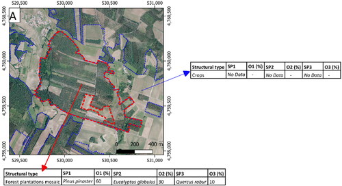
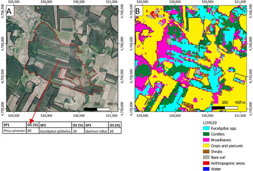
It should be emphasized that the species that are identified in a certain polygon with a certain level of occupancy are not geospatially delimitated. That is, their specific spatial location within the polygon is not given. An example of the MFE structure is shown in Figure 2. It shows two examples of polygons: A forest plantation mosaic (red) and a cropland polygon (blue). However, analyzing the PNOA image it is possible to see that both polygons contain crops and forest plantations. The red polygon is useful to exemplify the lack of information about the spatial distribution of the forest plantations within a polygon. The MFE only indicates that there are three species there but no how they are distributed within the polygon.

Figure 2. Detail of an MFE polygon and the corresponding attribute tables. Reference image: 2017 PNOA image (MTMAU 2022).

4. Methodology

4.1. Sentinel based map: the LCMG19

Sentinel-2 data were used to obtain the Land Cover Map of Galicia corresponding to 2019 (the LCMG19). The methodology described by Alonso et al. (2021) was used. It consists of a multitemporal analysis of a set of images, where each pixel is assigned to the most prevalent land cover class throughout the year. This approach minimizes misclassifications caused by the different spectral signatures of the different phenological stages of a species. The main steps are explained in this section.

First, the target land cover classes were defined. In this case, the classes corresponded to the most frequent land covers in Galicia: Eucalyptus spp., Conifers, Broadleaves, Shrubs, Crops and pastures, Bare soil, Anthropogenic areas, and Water bodies. Secondly, the time-series length was defined. To conduct the multi-temporal analysis, data from the entire year of 2019 was taken into consideration. Twelve images were used, one per month, in order to gather data that included the varying phenological stages of the vegetation throughout the year. The images were downloaded from the Copernicus Open Access Hub (ESA 2022). A threshold of 50% cloud cover was established. In cases where there were no images available for a given month that met this criterion, an image dating from the previous month or from the following month was selected. All the images were pre-processed to mask out the clouds using the 20 m cloud mask provided by the Sentinel-2 Level-2A product. The 10 m bands were resampled at 20 m using nearest neighborhood interpolation and the bands with a 60 m spatial resolution were discarded. The selection of the resolution and the bands is based on the indications of Alonso et al. (2021) methodology to automatically produce forest oriented land cover maps in Galicia. The pre-processing and the following described steps were done using R (R Core Team 2022).

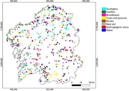
The training areas were defined through photointerpretation of the PNOA images 2017 and 2018 (MTMAU 2022) as well as in Alonso et al. (2021) study. A set of polygons of each land cover class were drawn over the PNOA images and over the whole Galician surface using the software QGIS (QGIS Development Team 2022). The land cover was identified over both images, 2017 and 2020, assuming that if the land cover agrees in both images the land cover of 2019 would agree as well. Google Street View images were used as a complement whenever it was possible to aid in the photointerpretation. Street View images were consulted in Google Maps (Google 2022). Figure 3 presents the distribution of the training polygons. The resulting training dataset was considered as a whole and was used for the classification in all of the tiles.

Figure 3. Distribution of the training polygons.

An independent supervised classification was performed for each image in the time-series. The algorithm used was Random Forest (RF), with a unique single model for all of the tiles comprising the study area, as described by Alonso et al. (2021). RF has been used successfully as well in another studies focused on producing land cover maps (Malinowski et al. 2020, Nasiri et al. 2022). Although there exist multiple of them RF tends to be selected due to its processing efficiency, robustness and ease of implementation (Swapan et al. 2020, Maxwell et al. 2018, Pelletier et al. 2016).

Finally, the annual map was generated. It was obtained through the aggregation of the single-date classifications. The criterion for assigning a given land cover class to a pixel consisted in selecting the most frequently identified class throughout the time-series (Plurality voting criterion (Lewinski et al. 2017, Alonso et al. 2021). The result was the final land cover map corresponding to 2019. The same procedure was applied for each of the Sentinel-2 tiles. The seven tiles were merged and clipped along the Galician borders to obtain one single map of the territory of Galicia.

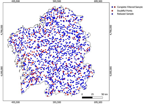
The map obtained was cross verified. A set of points were obtained following a simple random distribution across the Galician surface. Points corresponded to training polygon or pixels permanently covered by clouds were discarded. In total 1656 points were analyzed. The remaining set of points was deemed the complete filtered sample. The ground truth class of these points was obtained through photointerpretation of the PNOA images (MTMAU 2022). In cases where operators encountered problems or significant doubts when it came to assigning a class, points were marked as doubtful. A second verification dataset was built, called the reduced sample, where doubtful points were discarded. The distribution of the points is presented on Figure 4. To evaluate the map, two confusion matrixes were obtained for each of the two verification datasets: for the complete filtered sample and for the reduced sample. The following metrics were calculated: Overall Accuracy (OA), Producers Accuracy (PA), User’s Accuracy (UA), F1-Score, and Kappa Index.

Figure 4. Distribution of the verification points.

4.2. Map legend harmonization

The first step in comparing the LCMG19 with the MFE was to harmonize the legends of the two maps. The MFE polygons were filtered to include only those with data in the SP1 field, since these are the ones that correspond with areas that are mainly covered by trees. Then, the MFE tree species were combined into three groups since the LCMG19 has only three wooded classes. This process was performed by assessing information from the MFE’s data dictionary (MITERD 2011) and the description of the LCMG19 classes. The groups are described in Table 2, along with their corresponding LCMG19 classes. New attribute fields were created in the MFE table to specify the LCMG19 classes in each polygon that corresponded to the primary, secondary, and tertiary tree species. These were designated ESP1, ESP2, and ESP3 respectively. An example of the new attributes table of the MFE after harmonization is shown in Figure 5.

Figure 5. Example of the MFE attribute table after harmonization. Reference image: 2017 PNOA image (MTMAU 2022).

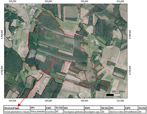
Table 2. Equivalences between the MFE tree species and the LCMG19 land cover classes.

Code of harmonized class	LCMG19 class	MFE species
1	Eucalyptus	Eucalyptus spp.
2	Conifers	Cedrus spp.
		Chamaecyparis spp.
		Cupressus spp.
		Other conifers
		Picea spp.
		Pinus spp.
		Pseudotsuga spp.
		Taxus spp.
		Thuja spp.
3	Broadleaves	Acacia spp.
		Acer spp.
		Ailanthus spp
		Alnus spp
		Arbutus spp.
		Betula spp.
		Castanea spp.
		Corylus spp.
		Crataegus spp.
		Fagus spp.
		Fraxinus spp.
		Ilex spp.
		Juglans spp.
		Laurus spp.
		Pistacia spp.
		Platanus spp.
		Populus spp.
		Prunus spp.
		Pyrus spp.
		Quercus spp.
		Robinia spp.
		Salix spp.
		Sorbus spp.
		Ulmus spp.

4.3. Map format harmonization

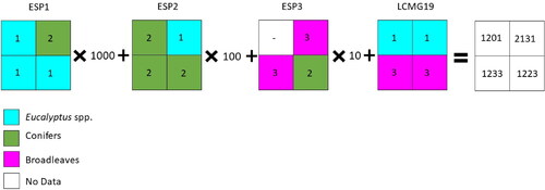
The spatial comparison of maps is accomplished through a pixel-to-pixel comparison. To perform this, the MFE map was transformed into raster format. Specifically, it was rasterized into three different raster layers: one for the primary species (ESP1), another for the secondary species (ESP2), and a third for the tertiary species (ESP3). In these layers, each pixel was coded according to its corresponding harmonized land cover class. The level of occupancy was not considered as the MFE does not include information regarding the spatial distribution of the species within a polygon.

In order to facilitate the comparison of the two maps, the three MFE raster layers were combined with the LCMG19 raster layer. This was done through arithmetic operations: each raster layer was multiplied by a factor of 10ⁿ and the sum of the resulting layers was taken (see Figure 6). The ultimate raster layer obtained compiled all of the information from the four layers: the primary, secondary, and tertiary tree species according to the MFE, and the land cover according to the LCMG19. This ultimate raster file was called the integrated raster file. This was identified as a very simple method to detect and quantify matches and mismatches among two maps. The factor 10ⁿ depends on the number of layers to compare. In this case it was needed to compare 4 layers, therefore one layer was multiplied by 1000, other by 100, other by 10 and the other one was not multiplied. It is important to remember for which factor you are multiplying each layer to be able to correctly interpret the integrated raster file.

Figure 6. Diagram of the procedure followed to compare the Spanish forest official cartography (the MFE) and the land cover map of Galicia produced using Sentinel-2 processing (the LCMG19). ESP1: the MFE raster layer containing the primary species (SP1) information, after legend harmonization. ESP2: the MFE raster layer containing the secondary species (SP2) information, after legend harmonization. ESP3: the MFE raster layer containing the tertiary species (SP3) information, after legend harmonization.

4.4. Comparison of Sentinel based map and the MFE

The maps were first evaluated visually, to analyze the capacity of each data source to map small stands. Then the area of wooded land use was estimated according to each map for the entire study area, and the results were compared. Finally, a pixel-to-pixel comparison was conducted to determine the level of agreement between the LCMG19 and the MFE in terms of mapping the spatial distribution of the different wooded land covers.

4.4.1. Net balance areas: Sentinel based map vs the MFE

The comparison of the areas of the different harmonized land use classes was performed for the entire Galician surface area as well as for each Galician province individually in order to investigate possible regional differences. For this purpose, the total area per harmonized class, as well as the total area of wooded land, was computed according to each of the two maps.

For the LCMG19, the estimation of areas was done by counting the number of pixels corresponding to each class and multiplying the result by the pixel size. For the MFE, the estimation was done by taking the sum of the areas of all of the polygons containing a certain class and applying a correction for the percentage of occupancy. For example, if the MFE has a polygon that says Eucalyptus globulus at 60% of occupancy as SP1 and Pinus pinaster at 40% of occupancy as SP2 the Eucalyptus surface contributed by that polygon is the 60% of the total polygon surface and the Conifers surface contributed by the same polygon is the 40% of the total polygon surface. This procedure was done to all the MFE polygons. The net balance comparison of the Sentinel based map and the MFE was accomplished through the comparison of the estimated areas covered by each harmonized class according to the two different maps.

4.4.2. Land use spatial distribution: Sentinel based map vs the MFE

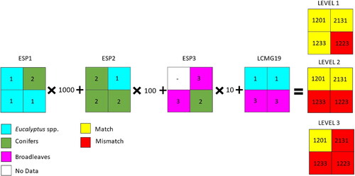
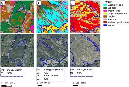
The spatial distribution of land use was compared between the two maps pixel-by-pixel, and pixel concordance was detected. Three levels of pixel concordance were distinguished: Level 1) The LCMG19 class matched any one of the ESP1, ESP2 or ESP3 layers; Level 2) The LCMG19 class matched either the ESP1 or the ESP2 layer; Level 3) The LCMG19 matched only the ESP1 layer. If, for example, ESP1 is Eucalyptus spp., ESP2 is Conifers, ESP3 is Broadleaves, and the LCMG19 class is Eucalyptus spp., this is a level 1 match. Figure 7 illustrates examples of different levels of matches. To detect the pixels that matched at each of the three levels for the entirety of Galicia, the integrated raster file, containing the information from the LCMG19 land cover classes and the MFE species with harmonized legends, was used. This file was evaluated quantitatively and qualitatively.

Figure 7. Spatial comparison of the LCMG19 and the MFE. Examples of Level 1, Level 2, and Level 3 matches.

The quantitative spatial comparison consisted of computing the percentage of matching pixels. This was done by taking the MFE as the reference source and the LCMG19 as the estimated source, and then vice versa. It was considered that none of the maps can be considered as the reference maps and that considering both as reference could allow to understand better the matches and mismatches. The percentages of matches were calculated for the three wooded classes separately as well as all together. Only the Level 1 matches were evaluated since this was the case where more matches will be expected. For example, using the MFE as the Reference map, and the LCMG19 as the estimated map, the concordance was computed as the percentage of pixels with a Level 1 match for a given class in both maps divided by the total number of pixels from that class in the MFE.

Finally, the spatial distribution of land use was evaluated visually. The integrated raster file provided a graphic representation of the matches and mismatches between the two maps at the three different levels. These representations allowed for the geographic distribution of wooded areas in Galicia to be evaluated, and they were obtained both as a whole and for each of the tree related classes individually.

5. Results

5.1. Sentinel based map results and verification

The land cover map obtained for Galicia in 2019 following the described methodology is shown in Figure 8. The complete filtered sample of points that was used for the verification was comprised of 1656 points, and the reduced sample of 1322 points. It should be highlighted that photointerpretation can be difficult to perform on randomly distributed points as there are instances where the operators encounter significant difficulties in interpreting the land cover. This is the case of pixels on the border of different land uses, as well as pixels in mixed forests amongst other circumstances. Such points were classified as doubtful and were removed from the complete filtered sample to form the reduced sample.

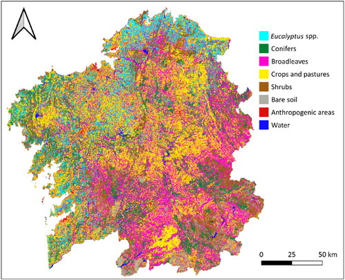
Figure 8. Land cover map of Galicia 2019 (LCMG19).

Table 3 shows the results for the cross verification performed using the complete filtered sample of verification points. Table 4 presents the results using the reduced sample of verification points. The OA obtained from both cross-verifications had a value of at least 80% and the KI was above 0.75. However, higher values were obtained when using the reduced sample: 6 percentage points higher for the OA and a KI 0.07 points higher. In general, class metrics (UA, OA, and F1 Score) were higher in the reduced sample. Nevertheless, both presented UA and PA accuracies around 70% or higher for all the tree related classes and an F1-Score of around 0.80. In the complete filtered sample, these values were lower when studying the PA and the F1-Score accuracy in the Shrubs class. In general, Bare soil and Anthropogenic areas presented lower accuracy metrics than vegetation-related classes.

Table 3. Confusion matrix obtained from the cross verification of the LCMG19 using the complete filtered sample.

Reference/ Classified	1	2	3	4	5	6	7	8	T	UA (%)
1	138	15	0	0	0	0	0	0	153	90
2	20	199	12	2	15	0	0	1	249	80
3	24	13	286	13	52	1	0	0	389	74
4	8	2	17	406	40	6	8	0	487	83
5	9	13	6	7	195	1	2	0	233	84
6	1	3	0	5	14	49	14	0	86	57
7	0	0	0	2	2	9	34	0	47	72
8	0	0	0	0	0	0	0	12	12	100
T	200	245	321	435	318	66	58	13	1656	OA (%)
PA (%)	69	81	89	93	61	74	59	92	OA (%)	80
F1 score	0.78	0.81	0.81	0.88	0.71	0.64	0.65	0.96	KI	0.75

Classes: Eucalyptus spp. (1), Conifers (2), Broadleaves (3), Crops and pastures (4), Shrubs (5), Bare soil (6), Anthropogenic areas (7) and Water (8). Metrics: User’s Accuracy (UA), Producer’s Accuracy (PA), Overall Accuracy (OA), T: Total, KI: Kappa Index.

Table 4. Confusion matrix obtained from the cross verification of the LCMG19 using the reduced sample.

Reference/ Classified	1	2	3	4	5	6	7	8	T	UA (%)
1	104	11	0	0	0	0	0	0	115	90
2	10	167	5	1	7	0	0	1	191	87
3	8	2	257	9	30	0	0	0	306	84
4	5	1	13	371	21	1	7	0	419	89
5	5	8	2	4	164	0	2	0	185	89
6	0	0	0	2	11	29	13	0	55	53
7	0	0	0	2	2	4	32	0	40	80
8	0	0	0	0	0	0	0	11	11	100
T	132	189	277	389	235	34	54	12	1322	OA (%)
PA (%)	79	88	93	95	70	85	59	92	OA (%)	86
F1 score	0.84	0.88	0.88	0.92	0.78	0.65	0.68	0.96	KI	0.82

Classes: Eucalyptus spp. (1), Conifers (2), Broadleaves (3), Crops and pastures (4), Shrubs (5), Bare soil (6), Anthropogenic areas (7) and Water (8). Metrics: User’s Accuracy (UA), Producer’s Accuracy (PA), Overall Accuracy (OA), T: Total, KI: Kappa Index.

5.2. Comparison of Sentinel based map and the MFE

5.2.1. Net balance areas: Sentinel based map vs the MFE

The results of the comparison of the net balance areas according to the LCMG19 and the MFE are shown in Tables 5 and 6. These tables include the differences in the estimations of the areas of the different land covers between the two data sources; these are provided in absolute and relative values. These results reveal that the LCMG19 and the MFE mainly differed in their estimation of the area covered by Broadleaves: according to the LCMG19 it was 56% higher than according to the MFE. The differences were greater in the western provinces: A Coruña and Pontevedra.

Table 5. Comparison of the LCMG19 and the MFE in terms of the surface area covered by the tree-related classes (in hectares).

Class	A Coruña (ha)	Lugo (ha)	Ourense (ha)	Pontevedra (ha)	Galicia (ha)
Eucalyptus	−48.455	−7.899	1.104	−21.827	−77.078
Conifers	−33.858	−55.043	−39.696	−24.594	−153.190
Broadleaves	86.566	88.984	41.591	48.921	266.062

Results are provided per province and for the whole region of Galicia.

Table 6. Comparison of the LCMG19 and the MFE in terms of the surface area covered by the tree-related classes (in percentage).

Class	A Coruña	Lugo	Ourense	Pontevedra	Galicia
Eucalyptus	−27%	−12%	88%	−35%	−25%
Conifers	−24%	−32%	−36%	−29%	−30%
Broadleaves	134%	44%	25%	109%	56%

Results are provided per province and for the whole region of Galicia.

The estimation of the area covered by conifers was also quite different in the two maps. According to the LCMG19, it was lower than according to the MFE, both for Galicia as a whole as well as for each of its provinces. The greatest difference in percentages was observed in Ourense, and the greatest absolute difference was in Lugo.

Finally, the area covered by Eucalyptus spp. in Galicia was smaller when it was estimated using the LCMG19 than when the MFE was used. However, in this case, it was noted that in Ourense, the province which traditionally has the least Eucalyptus logging, the LCMG19 reported much more area than the MFE, specifically 88% more, corresponding to 1.141 ha more. In the other provinces, the percentage differences ranged from −12% in Lugo to −35% in Pontevedra. The absolute differences ranged from −7.899 hectares in Lugo to −48.455 hectares in A Coruña, the province which traditionally has the most Eucalyptus logging.

5.2.2. Land use spatial distribution: Sentinel based map vs the MFE

The spatial comparison of the LCMG19 and the MFE at the three matching levels is presented from Figures 9 to 17. Matches and mismatches for Eucalyptus spp., Conifers and Broadleaves are presented separately. Eucalyptus spp. in Figures 9–11. Conifers in Figures 12–14. Broadleaves in Figures 15, 16 and 17. Eucalyptus spp. related figures reveal that in the case of the Eucalyptus spp., most of the hinterland of Lugo and Ourense was a mismatch, even when SP1, SP2 and SP3 were all considered. The mismatches were especially noticeable when the comparison was performed between the LCMG19 and SP1 of the MFE. In contrast, most of the matches were concentrated in the Northern coast of Lugo and A Coruña. This result confirms the numerical analysis.

Figure 9. Graphical representation of the spatial comparison of the Eucalyptus spp. distribution in the LCMG19 and the MFE Level 1: the LCMG19 vs the MFE considering SP1, SP2 and SP3. In green: pixel matches; in red: pixel mismatches.

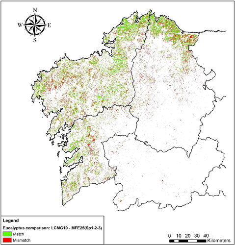
Figure 10. Graphical representation of the spatial comparison of the Eucalyptus spp. distribution in the LCMG19 and the MFE Level 2: the LCMG19 vs the MFE considering SP1 and SP2. In green: pixel matches; in red: pixel mismatches.

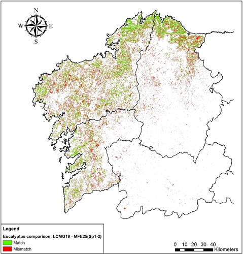
Figure 11. Graphical representation of the spatial comparison of the Eucalyptus spp. distribution in the LCMG19 and the MFE Level 3: the LCMG19 vs the MFE considering only SP1. In green: pixel matches; in red: pixel mismatches.

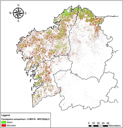
Figure 12. Graphical representation of the spatial comparison of the Conifers distribution in the LCMG19 and the MFE Level 1: the LCMG19 vs the MFE considering SP1, SP2 and SP3. In green: pixel matches; in red: pixel mismatches.

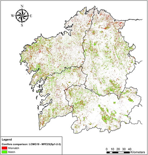
Figure 13. Graphical representation of the spatial comparison of the Conifers distribution in the LCMG19 and the MFE Level 2: the LCMG19 vs the MFE considering SP1 and SP2. In green: pixel matches; in red: pixel mismatches.

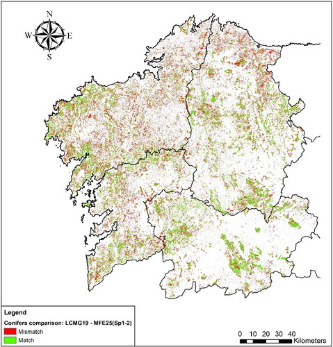
Figure 14. Graphical representation of the spatial comparison of the Conifers distribution in the LCMG19 and the MFE Level 3: the LCMG19 vs the MFE considering only SP1. In green: pixel matches; in red: pixel mismatches.

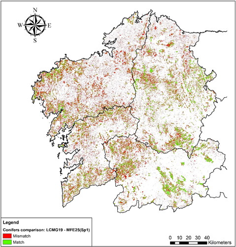
Figure 15. Graphical representation of the spatial comparison of the Broadleaves distribution in the LCMG19 and the MFE Level 1: the LCMG19 vs the MFE considering SP1, SP2 and SP3. In green: pixel matches; in red: pixel mismatches.

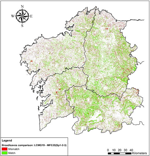
Figure 16. Graphical representation of the spatial comparison of the Broadleaves distribution in the LCMG19 and the MFE Level 2: the LCMG19 vs the MFE considering SP1 and SP2. In green: pixel matches; in red: pixel mismatches.

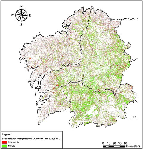
Figure 17. Graphical representation of the spatial comparison of the Broadleaves distribution in the LCMG19 and the MFE Level 3: the LCMG19 vs the MFE considering only SP1. In green: pixel matches; in red: pixel mismatches.

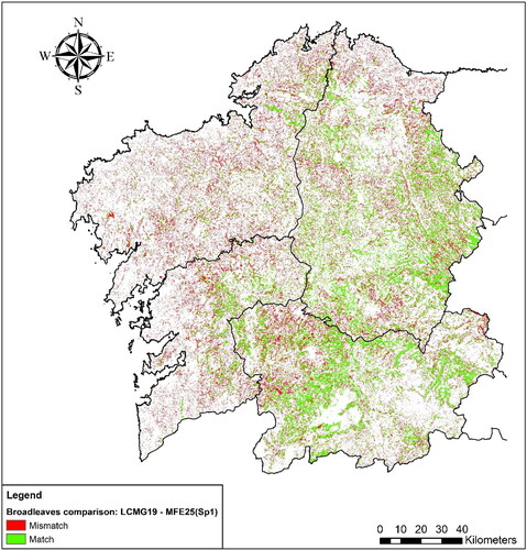
In the case of the Conifer figures, the mismatching areas were scattered throughout Galicia. Only a cluster of matching pixels was observed in the center of Ourense, even when only the SP1 layer was considered. Finally, the broadleaf maps show that mismatches arose all along the coastal borders of Galicia. Mismatches progressively decreased from the coast to the most interior parts of Galicia, as indicated in the quantitative analysis.

The maps with the geographical representation of the three levels of pixel matches and mismatches for the Galician woodland are presented in Figures 18–20. They clearly show that the majority of mismatches occur in coastal provinces, especially when the LCMG19 is compared only with SP1 from the MFE. This fact is in accordance with the logging activity.

Figure 18. Graphical representation of the spatial agreement of tree classes in the LCMG19 and the MFE. Comparison of the LCMG19 and the MFE considering SP1, SP2 and SP3. In green: pixel matches; in red: pixel mismatches.

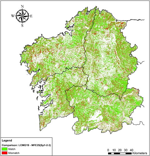
Figure 19. Graphical representation of the spatial agreement of tree classes in the LCMG19 and the MFE. Comparison of the LCMG19 and the MFE considering SP1 and SP2.In green: pixel matches; in red: pixel mismatches.

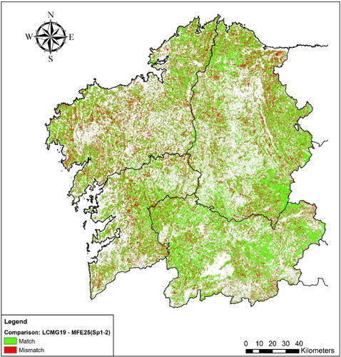
Figure 20. Graphical representation of the spatial agreement of tree classes in the LCMG19 and the MFE. Comparison of the LCMG19 and the MFE considering only SP1. In green: pixel matches; in red: pixel mismatches.

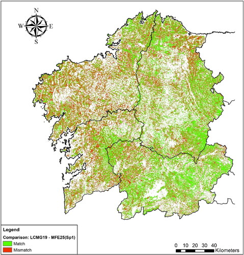
The results for the quantitative analysis of the spatial comparison are shown in Table 7. It presents as Reference the map that is considered to be the ground truth and as estimated: The map that is evaluated. They are provided separately for each province as well as for the whole surface area of Galicia, both for the three tree-related classes separately and for the overall wooded cover. The most salient results were the percentages of mismatches in tree-related classes. When the MFE was considered as the reference map, the comparison revealed that 34% of the pixels assigned to tree-related classes in the MFE did not correspond with a tree-related class in the LCMG19. Inversely, when the LCMG19 was considered as the reference map, 30% of the pixels corresponded to mismatches. Although the overall balance was similar, significant differences were found both when tree covers were analyzed individually, and when the provinces were analyzed separately.

Table 7. Quantitative results of the spatial comparison of the MFE and the LCMG19: percentages of matching pixels.

Area	Reference	Estimated	Eucalyptus match (%)	Conifers match (%)	Broadleaves match (%)	Tree cover match (%)
Galicia	MFE	LCMG19	58	55	79	66
	LCMG19	MFE	80	76	65	70
A Coruña	MFE	LCMG19	59	60	86	66
	LCMG19	MFE	86	75	53	70
Lugo	MFE	LCMG19	56	56	80	68
	LCMG19	MFE	71	77	68	71
Ponte vedra	MFE	LCMG19	57	53	87	64
	LCMG19	MFE	81	74	59	69
Ourense	MFE	LCMG19	40	50	74	66
	LCMG19	MFE	13	79	70	72

Reference: The map that is considered to be the ground truth. Estimated: The map that is evaluated.

According to the results, the percentages of matching pixels in the cases of Eucalyptus and Conifers were much higher when the LCMG19 was considered as the reference. These pixels may correspond to large areas where these land covers prevailed at the time of the creation of the MFE and remained intact when the Sentinel based map was generated. The opposite occurred with broadleaves: matching pixels were higher when the MFE was used as the reference. This result may indicate that the LCMG19 detected areas covered by broadleaves that were not detected in the MFE, something that had already been noted in the net balance comparison.

When analyzing the results per province, it could be seen that Ourense had a much lower percentage of matching pixels for Eucalyptus than the other provinces: 13% as opposed to 86% in A Coruña, 71% in Lugo and 81% in Pontevedra. This may be due to the new plantations that have arisen in recent years. Furthermore, Ourense is the province with the smallest differences between the reference source and the estimated source: in broadleaves the difference is between 74% and 70%.

6. Discussion

6.1. Sentinel based map

High accuracy metrics were obtained for the produced Sentinel-2 based map, the LCMG19. The accuracies are in line to the ones obtained in another similar Sentinel-2 based maps as for example Malinowski et al. (2020) which reported an overall accuracy of 78.7% and a KI of 0.75 for Spain. Accuracy metrics were lower when all of the points, as opposed to a reduced sample of points, were used for photointerpretation as there were many pixels where the ground truth could not be ensured. This raises the question of the appropriacy of using a random sample as opposed to a more flexible sample type that could minimize errors related to the identification of the ground truth. In any case, presenting both results allows the map user to follow the more conservative metrics using the metrics obtained from the complete filtered sample or to use the higher metrics, which ensure the ground truth, using the metrics obtained from the reduced sample. It should be mentioned that the accuracy metrics are lower than the ones obtained in Alonso et al. (2021) since in this study the verification points were distributed according to the recommended random distribution (Olofsson et al. 2012, Tsendbazar et al. 2021) while the sample used by Alonso et al. (2021) was biased to areas where the operator could easily perform the photointerpretation (Alonso et al. 2021). It should be mentioned that it is possible that two-storied high forests will be underrepresented in this map, since only the dominant leaf type will be identified. This may be a drawback of satellite imagery derived maps.

6.2. Maps format

The two maps compared greatly differed in terms of format, land cover legend, size of minimum mapping unit and update frequency. These differences posed a significant challenge when comparing maps. The first difficulty arose in dealing with the hierarchical structure of the MFE. It was observed that when only the primary species of the MFE was taken into account in the comparison with the Sentinel based map, the results differed greatly from when the secondary and tertiary species were also included. The differing spatial resolutions also posed a difficulty, especially because in the study area forest stands are often highly fragmented. The minimum mapping unit established by the MFE is 1 ha, meaning that in areas, like the study area, which have fragmented stands, numerous forest parcels are omitted from forest polygons. In fact, mismatches are much higher when SP2 and SP3 are not considered in the comparison. As a result of these mismatches, small parcels are overlooked when it comes to management and stocking prediction plans derived from the MFE data. The low spatial resolution of the MFE also hinders the detection of incipient land use dynamics. This represents an important drawback when dealing with changes from agricultural lands to forests as these kinds of changes are strictly regulated by law and in certain cases may need express permits (BOE 2021).

In contrast, an advantage of the MFE’s structure is that it defines forest units that are relatively stable in time. This is useful when defining which land surfaces are forests since a recently harvested area in a land cover map corresponds during a certain period of time with a non-tree related class (i.e. crops or pastures, bare soil or shrubs). According to FAO’s definition of forests, these areas should be considered forests as well (FAO, 2018). In fact, different studies have used remote sensing to overcome this issue (Wulder et al. 2020).

6.3. Map comparison

The visual inspection of the compared maps revealed that, as expected, the LCMG19 provides more details about the spatial distribution of forest resources than the MFE. Despite the medium resolution of the Sentinel images, the LCMG19 detects small forested areas that are not included in the MFE: small parcels, trees aligned along perimeters of parcels, and riverside vegetation, for example. An illustration of this is shown in Figure 21. Ottosen et al. (2020) have already reported that Sentinel-2 based maps could be more efficient on detecting trees outside what a NFI considers forests and that this can have a substantial effect when accounting tree cover in some specific regions. Galicia seems to be one of that regions.

Figure 21. Comparison between the MFE (A) and the LCMG19 (B).

The quantitative comparisons between the Sentinel based map and the MFE revealed that either the net estimated areas of land covers or their spatial distributions differs between the two maps. Firstly, the net balance indicates that eucalyptus and conifers differ between the maps. The graphical comparison of the two maps allowed for the interpretation of these differences. The LCMG19 may underestimate eucalyptus and conifers because areas with low canopy cover are classified as shrub pixels (Figure 22A). However, these areas are correctly classified as wooded areas in the MFE. This effect was also observed in Ganz et al. (2020) study, in what they call different forest definitions. Conversely, the MFE may overestimate these land covers since wooded polygons frequently include stand discontinuities such as forest roads or firebreaks (Figure 22A). These areas are correctly classified as artificial areas, shrubs or bare soil in the LCMG19. Finally, some divergences are due to land cover changes that occurred between the dates of production of the two maps, that is: logging areas (Figure 22B) and wildfires (Figure 22C). These limitations could explain why when the MFE is taken as the reference map only 66% of the wooded pixels match the wooded pixels on the LCMG19.

Figure 22. Examples of discrepancies between the MFE and the LCMG19.

Secondly, when the LCMG19 was considered as the reference map, the comparison revealed that 30% of pixels included in wooded classes were outside of wooded MFE polygons. The reason for this is likely the difference in the minimum mapping unit size between the two data sources. As it is 1 hectare in the MFE, small forest stands and tree lines, both very common phenomena in Galicia, may not be considered or included in forested polygons (see Figure 21). This pattern may be especially relevant in broadleaves, since they comprise the riparian forests, which are frequently long and narrow. Broadleaves, planted as lines of trees, are also often used to separate agricultural land properties. Finally, they are sometimes present in small abandoned land parcels. This observation was reinforced by the results of the net balance, which indicated that the MFE may underestimate broadleaves in comparison to the LCMG19. The temporal gap between the two data sources might also explain some divergences: new plantations, forest recuperation after a forest fire, and other such cases.

The analysis of the geographical distribution of matches and mismatches between the maps showed that most mismatches were in small patches distributed along the coastal areas. This pattern was expected since these areas are the ones with the most forestry activity (Xunta de Galicia 2022); the numerous logging events that occurred during the time gap between the creation of the two maps manifest as mismatches in the pixel to pixel comparison.

However, the two maps provided similar results for broadleaves in the province of Ourense, since, broadleaves are harvested with longer rotation cycles than other species, so a low frequency of update of the maps would be less relevant. Therefore, the update period of the MFE may be satisfactory for forest areas with very long rotation cycles and low rates of forest change, but a higher frequency of update is necessary to properly represent the forest land use distribution in areas with more transient forestry activity. This agrees with Gomez et al. 2019, the updating of the MFE is of special relevance in some specific areas.

In general, according to the presented results, it could be difficult to interpret which mismatches are due to the temporal gap between both maps and which related to the limitations of the maps. Therefore, it could be interesting to perform again a similar analysis when a new MFE map arises and compare it to a land cover map obtained in the same year of its production.

According to the results of this study, the production of remote sensing-based land cover maps could aid in automatically updating some of the MFE’s forest-related information, such as the presence of logging or wildfires. It can also be useful as a complement to the MFE to combat the problems discussed with the scale and the low frequency of update. However, when aiming to move forward, and working towards the integration of remote sensing data into the official Spanish cartography, consistency and interoperability issues must be resolved.

7. Conclusion

This study compares a forest-oriented land cover map obtained automatically using remote sensing imagery with the official forest cartography, a vector map obtained through photointerpretation. The obtained results highlight the possibilities that the automatic production of land cover maps using satellite imagery poses for complementing the official cartographical information in time periods between updates, although it was observed that non-broadleaved in early stages might be underrepresented. This is especially so in regions with extremely active forestry sectors. At the same time, it was observed that the production of such maps provides detailed, spatially explicit information about forest resource distribution in highly fragmented areas. However, it was observed that the integration of the two data sources with such different formats is challenging and can even lead to differing conclusions about forest resource estimations and distribution. When looking towards the future and aiming to integrate remote sensing data into the official Spanish cartography to aid in the ongoing monitoring of forests and their disturbances, consistency and interoperability issues must be solved. Some of the comparison approaches used in this study, such as the strategies followed to perform legend harmonization and spatial comparison, could be useful for a future integration of the official Spanish cartography with remote-sensing-based information. Such an integration could be a step towards producing internationally compatible forest information in the face of data incompatibilities similar to the ones encountered here. Indeed, such an action could possibly help Spain to be in line with the European Forest Agency’s (EFI, 2021) and the European Commission’s (Atzberger et al. 2018) calls for an integration and harmonization of European countries’ forest-related information.

Disclosure statement

No potential conflict of interest was reported by the author(s).

Data availability statement

The data that support the findings of this study are available from the corresponding author, J.A, upon reasonable request.

Additional information

Funding

This work was supported by the administration of rural areas of the government of Galicia ‘Continuous forestry inventory of Galicia’ under grant 2020CONVINVENTARIOFORESTALR002; Spanish ministry of Sciences, Innovation and Universities under grant FPU19/02054; Spanish Ministry of Sciences, Innovation and Universities under grant PID2019- 111581RB-I00 project PALEOINTERFACE: STRATEGIC ELEMENT FOR THE PREVENTION OF FOREST FIRES, DEVELOPMENT OF MULTISPECTRAL AND 3D ANALYSIS METHODOLOGIES FOR INTEGRATED MANAGEMENT. Additionally, it benefits from the aid of the Teaching Innovation Group ‘ODS Cities and Citizenship’ of the University of Vigo.

References

- Alonso L, Picos J, Amesto J. 2021. Forest land cover mapping at a regional scale using multi-temporal Sentinel-2 imagery and RF models. Remote Sens. 13:2237.
- Arenas S, Rodríguez-Soalleiro R, Diaz-Balteiro L. 2019. Turno óptimo de Eucalyptus nitens en Galicia introduciendo la fiscalidad en el análisis. XII Congreso de Economía Agraria.
- Atzberger C, Zeug G, Defourny P, Aragão L, Hammarström L, Immitzer M. 2018. Study on monitoring of forests through remote sensing. Luxemburg. European Comission.
- Barrett F, McRoberts RE, Tomppo E, Cienciala E, Waser LT. 2016. A questionnaire-based review of the operational use of remotely sensed data by national forest inventories. Remote Sens Environ. 174:279–289.
- Costa H, Benevides P, Marcelino F, Caetano M. 2020. Introducing automatic satellite image processing into land cover mapping by photo-interpretation of airborne data. Int Arch Photogramm Remote Sens Spatial Inf Sci. XLII-3/W11:29–34.
- BOE. 2021. Ley 11/2021, de 14 de mayo, de recuperación de la tierra agraria de Galicia. BOE núm. [Galician agricultural lands restoration law] 152, de 26 de junio de 2021, p. 76801 a 76926.
- Büttner G, Kosztra B, Soukup T, Langanke T. 2017. CLC18 Technical Guidelines. Austria: European Environment Agency.
- [EFI] European forest Institute. 2021. EFI Network Fund, Towards A Harmonised European Forest Monitoring System. [accessed 2022 Jun 08]. https://efi.int/grants-training/grants/G-01-2021.
- [ESA] European Space Agency. 2015. Sentinel-2. [accessed 2022 Jun 22]. https://www.esa.int/Space_in_Member_States/Spain/SENTINEL_2.
- [ESA] European Space Agency. 2022. Copernicus and European Comission. Copernicus Open Access Hub. [accessed 2022 Jun 22]. https://scihub.copernicus.eu/dhus/#/home.
- [FAO] Food and Agriculture Organization. 2017. Voluntary guidelines on National Forest Monitoring. ISBN 978-92-5-109619-2
- [FAO] Food and Agriculture Organization. 2018. Global forest resources assessment 2020. Terms and Definitions. Forest Resources Assessment Working Paper 188, Rome
- [FAO] Food and Agriculture Organization. 2020. Better data, better decisions – Towards impactful forest monitoring. Forestry Working Paper, 16.
- [FISE] Forest Information System for Europe. 2022. Forest Information system for Europe. [accessed 2022 Jun 08]. https://forest.eea.europa.eu/.
- Ganz S, Adler P, Kändler G. 2020. Forest cover mapping based on a combination of aerial images and Sentinel-2 satellite data compared to national forest inventory data. Forests. 11:1322.
- Gomez CAP, Hermosilla T, Montes F, Pascual C, Ruiz L, Alvarez-Taboada F, Tanase M, Valbuena R. 2019. Remote sensing for the Spanish forests in the 21st century: a review of advances, needs and opportunities. For Syst. 28(1):eR001.
- Google. 2022. Google Maps. [accessed 2022 Sep 16]. google.es/maps/?hl=es.
- [IGE] Instituto Galego de Estatística. 2020. Explotacións por tipo de cultivo. Distribución segundo a SAU. [accessed 2023 Feb 06] https://www.ige.gal/igebdt/esqv.jsp?ruta=verTabla.jsp?OP=1&B=1&M=&COD=10331&R=9915[12];1[0]&C=0[1]&F=&S=2:2020&SCF=.
- Inglada J, Vincent A, Arias M, Tardy B, Morin D, Rodes I. 2017. Operational high resolution land cover map production at the country scale using satellite image time series. Remote Sens. 9(1):95.
- Lang M, Kaha M, Laarmann D, Sims A. 2018. Construction of tree species composition map of Estonia using multispectral satellite images, soil map and a random forest algorithm. For Stud. 68(1):5–24.
- Levers C, Verkerk H, Müller D, Verburg P, Butsic V, Leitão P, Lindner M, Kuemmerle T. 2014. Drivers of forest harvesting intensity patterns in Europe. For Ecol Manage. 315:160–172.
- Lewinski S, Nowakowski A, Malinowski R, Rybicki M, Kukawska E, Krupinski M. 2017. Aggregation of Sentinel-2 Time Series Classifications as a Solution for Multitemporal Analysis. In Proceedings Volume 10427, Image and Signal Processing for Remote Sensing XXIII, SPIE Remote Sensing: Warsaw, Poland.
- Malinowski R, Lewiński S, Rybicki M, Gromny E, Jenerowicz M, Krupiński M, Nowakowski A, Wojtkowski C, Krupiński M, Krätzschmar E, et al. 2020. Automated production of a land cover/use map of Europe based on Sentinel-2 Imagery. Remote Sens. 12:3523.
- Maxwell AE, Warner TA, Fang F. 2018. Implementation of machine-learning classification in remote sensing: an applied review. Int J Remote Sens. 39:2784–2817.
- [MITERD] Ministerio para la Transición Ecológica y el Reto Demográfico, Gobierno de España. 2011. Mapa forestal Español (MFE) de máxima actualidad. [accessed 2022 Jun 08] https://www.miteco.gob.es/es/cartografia-y-sig/ide/descargas/biodiversidad/mfe.aspx.
- [MITERD] Ministerio para la Transición Ecológica y el Reto Demográfico. 2018. Anuario de estadística forestal. [accessed 2022 Jun 21]. https://www.mapa.gob.es/es/desarrollorural/estadisticas/aef_2018_documentocompleto_tcm30- 543070.pdf
- [MTMAU] Ministerio de Transporte Movilidad y Agenda Urbana. 2022. Plan Nacional de Ortofotografía Aérea (PNOA). [accessed 2022 June 22]. https://pnoa.ign.es/.
- [MTMAU and IGN] Ministerio de Transporte Movilidad y Agenda Urbana and Instituto Geográfico Nacional. 2022. Centro de Descargas. Centro Nacional de Información Geográfica. [accessed 2022 June 22]. http://centrodedescargas.cnig.es/CentroDescargas/index.jsp.
- Nasiri V, Deljouei A, Moradi F, Sadeghi SMM, Borz SA. 2022. Land use and land cover mapping using Sentinel-2, Landsat-8 satellite images, and Google Earth Engine: a comparison of two composition methods. Remote Sens. 14(9):1977.
- Nomura K, Mitchard ETA. 2018. More than meets the eye: using Sentinel-2 to map small plantations in complex forest landscapes. Remote Sens. 10(11):1693.
- Olofsson P, Stehman SV, Woodcock CE, Sulla-Menashe D, Sibley AM, Newell JD, Friedl MA, Herold M. 2012. A global land-cover validation data set, part I: fundamental design principles. Int J Remote Sens. 33:5768–5788.
- Ottosen TB, Petch G, Hanson M, Skjøth CA. 2020. Tree cover mapping based on Sentinel-2 images demonstrate high thematic accuracy in Europe. Int J Appl Earth Obs Geoinf. 84:101947.
- Pelletier C, Valero S, Inglada J, Champion N, Dedieu G. 2016. Assessing the robustness of random forests to map land cover with high resolution satellite image time series over large areas. Remote Sens. Environ.187:156–168.
- QGIS Development Team. 2022. QGIS Geographic Information System. Open Source Geospatial Foundation Project. [accessed 2022 Sep 16]. https://qgis.org/es/site/.
- R Core Team 2022. R: a Language and environment for statistical computing. Vienna, Austria: R Foundation for Statistical Computing. https://www.R-project.org.
- Rodríguez Quitán MA, Ramil-Rego P. 2007. Clasificaciones Climáticas Aplicadas a Galicia: revisión desde una Perspectiva Biogeográfica. Recursos Rurais. 3:31–53.
- Spanish Government. 2011. Ministerio de Hacienda. Sede Electrónica del Catastro. [accessed 23 July 2021]. https://www.sedecatastro.gob.es.
- Swapan T, Singha P, Mahato S, Shahfahad PS, Liou Y, Rahman A. 2020. Land-Use Land-Cover Classification by Machine Learning Classifiers for Satellite Observations—A Review. Remote Sensing. 12:1135.
- Szantoi Z, van de Kerchove R, Tsendbazar NE, Herold M. 2021. Next generation land cover monitoring services: towards a flexible, user-oriented approach. IEEE International Geoscience and Remote Sensing Symposium IGARSS, p. 2070–2073.
- Szantoi Z, Geller GN, Tsendbazar N, See L, Griffiths P, Fritz S, Gong P, Herold M, Mora B, Obregón A. 2020. Addressing the need for improved land cover map products for policy support. Environ Sci Policy. 112:28–35.
- Tolosana E, Diaz-Balteiro L, Lobo-Huici E. 2017. Estudio del turno óptimo de Eucalyptus globulus en el norte de España. VII Congreso Forestal Español. ISBN 978-84-941695-2-6 .
- Tsendbazar N, Herold M, Li L, Tarko A, de Bruin S, Masiliunas D, Lesiv M, Fritz S, Buchhorn M, Smets B, et al. 2021. Towards operational validation of annual global land cover maps. Remote Sens Environ. 266:112686.
- Wulder M, Hermosilla T, Stinson G, Gougeon FA, White JC, Hill DA, Smiley BP. 2020. Satellite-based time series land cover and change information to map forest area consistent with national and international reporting requirements. For: An Int J For Res. 93:3–343.
- Wulder MA, Coops NC, Roy DP, White JC, Hermosilla T. 2018. Land Cover 2.0. Int J Remote Sens. 39:4254–4284.
- Xunta de Galicia. 2016. 1a revisión del plan forestal de Galicia. Documento diagnóstico del monte y el sector forestal gallego. [accessed 2022 Jun 22]. https://mediorural.xunta.gal/sites/default/files/temas/forestal/plan-forestal/1_revision_plan_forestal_cast.pdf.
- Xunta de Galicia. 2021. 1a Revisión del plan forestal de Galicia. Hacia la neutralidad carbónica. Xunta de Galicia. Consellería do Medio Rural. Santiago de Compostela.
- Xunta de Galicia. 2022. Sistema de indicadores da administración dixital. Producción forestal. [accessed 2022 June 22]. https://indicadores-forestal.xunta.gal/portal-bi-internet/dashboard/Dashboard.action?selectedScope=OBSFOR_BI_A02_INT&selectedLevel=OBSFOR_BI_2_INT.L0&selectedUnit=12&selectedTemporalScope=2&selectedTemporal=31/12/2020.