A comparative study on the applicability and effectiveness of NSVI and NDVI for estimating fractional vegetation cover based on multi-source remote sensing image

Abstract

Fractional vegetation coverage (FVC) is an important ecological parameter reflecting the growth of regional plants. Existing FVC estimation is often based on vegetation indices, especially the Normalized Difference Vegetation Index (NDVI). However, NDVI can be oversaturated and easily affected by problems such as ‘shadow’ in images, which leads to a decrease in the precision of FVC estimation. In this study, the Normalized Shaded Vegetation Index (NSVI) was used to comprehensively compare the estimation ability of FVC with NDVI, and the differences in FVC estimation ability between NSVI and NDVI were explored. Based on two dimensions of ‘bright’ and ‘shadow’ hierarchies and FVC ranks, four evaluation systems of signal-to-noise ratio (SNR), index range, statistical model and dimidiate pixel model were selected from Sentinel-2A MSI, Landsat-8 OLI and Resource-1-02D (ZY1-02D) images and covered a variety of topographic landscapes. The results showed that: (1) the ability of NSVI to resist soil background is slightly smaller than NDVI; (2) the range of NSVI and NDVI in hyperspectral images is slightly larger than multispectral images, and the ability of NSVI to detect vegetation information in medium-high-rank and high-rank FVC areas has obvious advantages; (3) in the same kind of regression model, the goodness of fit of NSVI, NDVI and FVC was slightly higher in bright areas than in shaded areas, and the goodness of fit of the five regression models obtained from NSVI showed a significant advantage in bright areas compared with NDVI, with the best fit of the cubic curve model; (4) the estimation accuracy of the dimidiate pixel model based on NSVI and NDVI is slightly higher in bright areas than in shaded areas, and the estimation ability of NSVI is slightly better than that of NDVI in bright areas with medium-high-rank and high-rank FVC. NSVI and NDVI have their own advantages in SNR, index range, statistical model and dimidiate pixel model, so it is suggested that when remote sensing estimation of FVC is carried out, NSVI should be preferred in medium-high-rank and high-rank FVC areas, and NDVI should be preferred in low-rank FVC areas in shaded areas.

HIGHLIGHTS

• Comparing FVC estimation ability in bright and shaded areas of multi-source images

• Effectiveness of NSVI and NDVI for estimating FVC are better in bright areas

• NSVI is preferred in areas with MH-rank and H-rank FVC

• NDVI is preferred in areas with L-rank FVC in shaded areas

• NSVI has broader application and improvement prospects in estimating FVC

Keywords:

• Fractional vegetation coverage
• dimidiate pixel model
• capability differences to detect vegetation information
• bright and shaded areas

1. Introduction

FVC is the percentage of the vertically projected area of vegetation (including leaves, stems and branches) on the ground to the total area of the statistical area (Leprieur et al. 2000; Gitelson et al. 2002). It reflects the area where plants carry out photosynthesis and the luxuriant degree of vegetation growth, and can reflect the growth status and trend of vegetation to a certain extent (Carlson et al. 1994; Owen et al. 1998; Li et al. 2004; Zhao et al. 2019). Large-scale estimation and monitoring of vegetation cover has important value and significance for climate change, ecosystem modeling, vegetation phenology, land use management fields and other related terrestrial studies (Hirano et al. 2004; Andrew et al. 2013; Hansen et al. 2014; Crowther et al. 2015; Pudmenzky et al. 2015).

In the process of vegetation remote sensing estimation, there are two hierarchies of ‘bright’ and ‘shadow’ on remote sensing images due to the combined effects of solar incidence angle, terrain undulation and the height of the features themselves. The shaded areas reduce the amount of information on the target features on remote sensing images, which greatly interferes with the work of feature identification, information extraction and quantitative algorithm construction (Silvoster and Govindan 2012; Shen and Ji 2016; Vupparaboina et al. 2018; Chen et al. 2019; Dong et al. 2019), so the different vegetation indices in the two hierarchies of ‘bright’ and ‘shadow’ have different effects. These differences can influence the estimation of FVC (Rundquist 2002; Liu et al. 2014; Song et al. 2017). Among many vegetation indices, NDVI is one of the most popular vegetation indices because of its responsiveness to FVC changes, however, when NDVI is applied for land degradation detection, its ability to identify low-coverage vegetation or real ground information in shaded areas is slightly inferior and its response-ability is not sensitive enough (Gunasekara et al. 2015). Otherwise, NDVI values will be larger in shaded areas, and the accuracy of estimated FVC will be reduced due to the effect of shadow, while in high cover vegetation detection applications, NDVI suffers from oversaturation and is also affected by shadow, resulting errors in detecting vegetation information (Huete 1988; Huete et al. 2002; Gunasekara et al. 2015; Zhang et al. 2015; Jiang et al. 2019; Jiao et al. 2020). Therefore, the NDVI-based FVC estimation is theoretically inevitable to exist information errors in shaded areas. Related scholars had improved vegetation information extraction methods to compensate for the shortcomings of NDVI's ability to detect vegetation. For example, Ono et al. constructed the Shadows Index (SI) to improve the accuracy of vegetation detection in shaded areas (Ono et al. 2010); Xu et al. proposed the Normalized Shaded Vegetation Index (NSVI) to further enlarge the difference between vegetation in shaded areas and vegetation in bright areas and water areas, and enlarge the spectral differences of typical features and improving the separability of spectrally confusing elements which can compensate the deficiencies of vegetation information detected by NDVI to some extent (Xu et al. 2013, 2018; Hu et al. 2021). However, few scholars have studied the applicability of index estimation of FVC from the perspective of different hierarchies of ‘bright’ and ‘shadow’ and different FVC ranks, therefore, it is crucial to explore the applicability of vegetation index in the process of FVC estimation in different ranks and establish an accurate remote sensing estimation model for regional FVC.

The aim of this study is to explore the applicability and effectiveness of NSVI and NDVI in estimating FVC, the differences of the ability of NSVI and NDVI to eliminate soil background, the differences of the ability to detect vegetation information, and the differences of FVC estimation accuracy in the constructed statistical model and dimidiate pixel model of multi-type image data sources in bright and shaded areas. Ultimately, establishing an accurate and efficient remote sensing estimation model of FVC and providing a reference for FVC estimation studies of vegetation indices.

2. Materials and methods

2.1. Test images and samples

2.1.1. Satellite images selection and processing

There exist differences in the radiometric response of different sensors to the same band and the reflection of feature information (Barsi et al. 2018; Arekhi et al. 2019; Chastain et al. 2019; Mancino et al. 2020), and in order to reflect the scientific and universality of the index’s comparison, three image data sources, Sentinel-2A, Landsat-8 OLI and Resource 1 02D (ZY1-02D) in Figure 1, covering different topographic and geomorphological regions in Fujian Province, China, were used in this study. Sentinel-2A data is a subsatellite of the European Copernicus Program that undertakes multispectral high resolution, which was launched on 23 June 2015 with a 13-band MSI imaging sensor covering the visible to short-wave infrared bands with an efficient revisit cycle of 10 days (Li et al. 2018; Guzinski and Nieto 2019). It is freely available worldwide since 2016 (https://scihub.copernicus.eu/). Sentinel-2A data is characterized by high spatial resolution, short revisit period and wide coverage of wavelength range. In order to maintain the original characteristics of the image spectral values, radiometric calibration and atmospheric correction of the images were performed with Sen2cor plug-in to obtain L2A-level reflectance data that best reflect the underlying atmosphere. The Landsat-8 OLI satellite was launched by an Atlas-V rocket on 11 February 2013. The satellite carries the sensors of Operational Land Imager (OLI) and Thermal Infrared Sensor (TIRS). Landsat-8 orbits the Earth in a sun-synchronous near-polar orbit with an altitude of 705 km and an inclination angle of 98.2°, completing an Earth orbit every 99 m with a repetition period of 16 d and collecting 550 scenes per day. In this study, the Landsat-8 OLI was processed for radiometric calibration and atmospheric correction. ZY1-02D was successfully launched on 12 September 2019, built under the auspices of the Ministry of Natural Resources of China and is a medium-resolution remote sensing operational satellite for space-based planning. The satellite works in a sun-synchronous orbit with a return period of 55 days. In this study, radiometric calibration, atmospheric correction and orthorectification correction processing were performed on ZY1-02D with ENVI 5.6 software. The specific parameters such as imaging time of the above three image data sources are shown in Table 1. Because the presence of water areas in some data will affect the subsequent FVC calculation, it is necessary to mask the image to avoid the influence of water during the research process. The specific process is to use ENVI5.3 to remove the areas of three images with NDVI values less than 0 by the ‘mask’ tool.

Figure 1. Test image selection. In order to reflect the scientific rationality and universality of the experiment, the selected test images include both multispectral and hyperspectral image data, as well as coastal areas, high mountains and hills, plains and other different topographical and geomorphological areas.

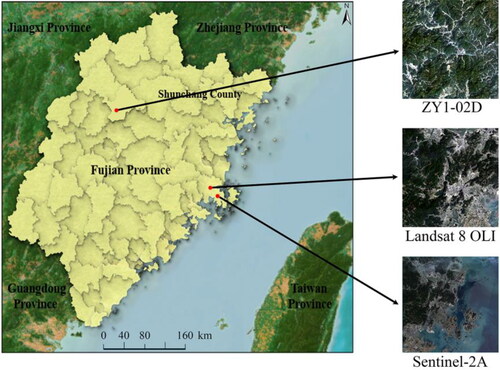
Table 1. Test image related parameters.

Satellite image	Time	Spatial resolution	Spectral range	Number of bands
Sentinel-2A	2020-04-13	10 m	400–2400 nm	13
Landsat-8 OLI	2020-04-23	30 m	433–2300 nm	7
ZY1-02D	2021-02-18	30 m	400–2500 nm	166

2.1.2. Samples and analysis dimensions selection

In this study, 238 region of interest (ROIs) of 10 m × 10 m, 232 ROIs of 30 m × 30 m and 193 ROIs of 30 m × 30 m were evenly selected on the acquired Sentinel-2A, Landsat-8 OLI and ZY1-02D images according to the preliminary field investigation, respectively, and the corresponding NDVI and NSVI values of each sample point were obtained by waveband calculation. Secondly, the sample areas of Sentinel-2A and Landsat-8 OLI were imported into Google Earth software, and since Google Earth does not have images of ZY1-02D that accurately correspond to the time period, so the fused Gaofen-1 (GF-1) PMS satellite image with 2 m resolution was used as the validation data of ZY1-02D image data. Photoshop and manual visual interpretation were used to obtain the FVC of each sample point, which was regarded as the true value of FVC, and the ArcGIS hillshade model combined with visual interpretation was used to acquire the accurate positions shaded areas in the study area (Zhang et al. 2021). Finally, in order to reduce the human visual interpretation error, after every two persons interpreted the preliminary results, the third person reviewed and corrected them, and the true FVC value was taken as the corrected mean value.

In this study, considering two dimensions of ‘bright’ and ‘shadow’ hierarchies and FVC ranks, 152 samples in bright areas and 86 samples in shaded areas were collected in Sentinel-2A, 147 samples in bright areas and 85 samples in shaded areas were collected in Landsat-8 OLI, 87 bright samples in areas and 106 samples in shaded areas were collected in ZY1-02D. The sample sites to be analyzed were divided into five ranks according to the vegetation coverage: low-rank FVC areas (less than 20%), medium-low-rank FVC areas (20–40%), medium-rank FVC areas (40–60%), medium-high-rank FVC (60–80%) and high-rank FVC (80–100%; Cui et al. 2013; Liu et al. 2022). Because the spatial resolution of Google Earth images of this test area is as high as 4 m in most areas and 2 m in local areas, the results of this interpretation can be regarded as true values (Table 2).

Table 2. Examples of areas with each rank of vegetation coverage under bright and shaded hierarchies.

FVC rank	Hierarchy	Reference ratio (%)	Hierarchy	Reference ratio (%)
	Bright		Shadow
Low		12.36		19.83
Medium-Low		26.52		30.45
Medium		45.28		44.80
Medium-High		60.01		62.52
High		87.43		91.04

2.2. Construction principles of NSVI and NDVI

When comparing the FVC estimation ability of both NSVI and NDVI, it is important to start from the background and principle of their constructions. The construction of vegetation indices using a combination of red and near-infrared bands is a practical and effectual method to acquire vegetation information from multispectral remote sensing image data (Tian and Min 1998). NDVI is the most widely used vegetation index (Rouse et al. 1973), however, NDVI can be oversaturated in areas with high-rank vegetation cover and is susceptible to problems such as ‘shadow’ in images, which leads to inaccurate detection of vegetation information (Yang et al. 2013; Liu et al. 2018). For this, Xu et al. established the Shaded Vegetation Index (SVI) from the spectral difference between vegetation and other features in shaded areas of mountain hills, and further constructed the Normalized Shaded Vegetation Index (NSVI) by using Landsat TM/ETM+, ALOS AVNIR-2, CBERS-02B-CCD, HJ-1-CCD, etc., to verify its detection effect (Xu et al. 2013, 2018). In addition, Garyson et al. constructed the same model as NSVI in 2017 to estimate terrestrial Gross Primary Productivity (GPP); Lee et al. demonstrated that the enhancement of precision of the UAV nitrogen inversion model could be achieved by shadow removal from NSVI, all of which reflected the potential and strengths of NSVI in several fields of application (Li et al. 2021). In terms of the construction perspective of the index, NSVI is constructed by multiplying NDVI with the NIR band, which can ensure the absolute difference between the vegetation in bright areas, the vegetation in shaded areas and the water areas in the NIR band, and also amplify NDVI to eliminate the possible confusion in the image pixels. Therefore, theoretically, NSVI may compensate for the deficiencies of NDVI in estimating FVC to a certain extent and improve the estimation accuracy of FVC as a whole. However, NSVI was proposed mainly for mountains and hills, and did not consider non-forested areas such as built-up areas, therefore, whether the vegetation detection capability of NSVI is superior to NDVI in all aspects? In this study, the FVC estimation capability of NSVI and NDVI will be explored and verified based on their respective applicability and advantages. The formulas for NDVI, SVI and NSVI are as follows: (1) $$\text{NDVI}=\left(\text{NIR}\text{-}\mathrm{R}\right)/\left(\text{NIR}+\mathrm{R}\right)$$(1) (2) $$\text{SVI}=\text{NIR}\mathrm{\times }\left(\text{NIR}\text{-}\mathrm{R}\right)/\left(\text{NIR}+\mathrm{R}\right)$$(2) (3) $$\text{NSVI}=\left(\text{SVI}-\text{SV}{I}_{\min }\right)/\left({\text{SVI}}_{\max }-\text{SV}{I}_{\min }\right)$$(3) where NIR represents the reflectance of the NIR band; R represents the reflectance of the red band; SVI_max is the maximum value of SVI; SVI_min is the minimum value of SVI.

2.3. Analysis of vegetation information detection ability of the indices

2.3.1. Signal-to-noise ratio

When ground surface is not completely covered by vegetation, part of infrared light is scattered or transmitted to the ground surface when it passes through the vegetation canopy, and complex soil–vegetation interactions occur, which are reflected to the sensor with both vegetation and soil background information, causing errors during the application of vegetation extraction. Qi et al. introduced a statistical indicator called the vegetation signal–soil noise ratio, or signal-to-noise ratio (S/N, SNR) (Qi et al. 1994), which is calculated as follows: (4) $$\mathrm{S}/\mathrm{N}=\overline{\text{VI}}/2\mathrm{\delta }$$(4) where $\overline{VI}$ represents the mean value of vegetation indices measured based on the same vegetation conditions; δ is the standard deviation of VI change.

SNR is a comprehensive index reflecting the changes of vegetation index and soil background, which reflects the complex spectral changes in the process of vegetation–soil interaction, and the influence of soil background spectrum on vegetation index is closely related to the changes of vegetation information. For the same image, different vegetation conditions have different vegetation-soil interaction processes and results, so the S/N values calculated for different VIs are different, and the actual meaning expressed is not consistent with the trend direction and vice versa. The larger the S/N value, the stronger the VI's ability to eliminate soil impacts, and the stronger the ability to extract vegetation information, and the weaker the vice versa.

2.3.2. Range of index values

The range of index reflects the feedback and estimation ability of each vegetation index for different ranks of FVC, and the change in the range of indices under different ranks is also an important factor reflecting its ability to detect vegetation information. For the same rank of FVC, the larger the range of vegetation index values, the more sensitive it is to vegetation details changes (Zhang 2016), which indicates that the vegetation index has a better capability to detect vegetation information, and vice versa.

2.4. Estimation model and evaluation of FVC

2.4.1. Statistical model

The correlations between vegetation indices and FVC can not only show the sensitivity of the indices to vegetation information and reflect their ability to estimate FVC to a certain extent, but also provide some reference for the construction of the related model. In this study, Spearman’s correlation method was used for analytical sensitivity for each vegetation index to FVC by using the correlation between the index and FVC. When the correlation between indices and FVC is larger and positive, the Spearman correlation coefficient is closer to positive 1, which proves that the indices are more sensitive to reflect FVC, and vice versa, and the specific principle is as follows: (5) $${\rho }_{\sigma }=1-\frac{6\sum _{t=1}^v{D}_l^2}{v\left(v^2-1\right)},\sum _{i=1}^n{D}_i^2=\sum _{i=1}^n{\left(U_i-V_i\right)}^2$$(5) where U_i and V_i are the ranks of the two variables ranked by size or superiority, respectively, and n is the number of variables. The Spearman correlation coefficient is not directly obtained from the calculated variables, but is calculated using the rank, which is essentially a nonparametric method, independent of the sample size and the distribution of the variables, but only related to the ranking of the variables. The Spearman correlation coefficient takes values in the interval [−1,1].

Based on correlation analysis, the primary linear, quadratic, cubic, exponential, logarithmic, multiplicative power and multivariate linear regression statistical models were developed for training sample points using the true FVC values and their corresponding NSVI and NDVI values. The effectiveness of the estimation model is judged by the coefficient of determination R² and the statistical p-value in the statistical model. The coefficient of determination of the model, R², takes values in the range of [0, 1], and when R² is closer to 1, it means that the model fits with higher accuracy and vice versa. The statistical p-value is an indicator to test whether the correlation between variables is significant, 0.01 < p < 0.05 indicates that the correlation between variables is significant, and p < 0.01 indicates that the correlation between variables is highly significant. The formula of each model is shown in Table 3.

Table 3. Model calculation formula.

Model categories	Calculation formula
Primary linear model	FVC = ax + b
Quadratic linear model	FVC = ax^2 + bx + c
Cubic linear model	FVC = ax^3 + bx^2 + cx + d
exponential model	FVC = ae^bx
Logarithmic model	FVC = alnx + b
Power Models	FVC = a1x1 + a2x2 + … + anxn + b

Note: x is the value of the vegetation index; a, b, c and d are the undetermined coefficients of the model, respectively.

2.4.2. Dimidiate pixel model

FVC is usually constructed using an index to construct a dimidiate pixel model, which is the simplest and most commonly used model for linear pixel decomposition assuming that the image pixel is composed of two components, non-vegetation and vegetation and the spectral information is linearly combined by them. The FVC value of each pixel is obtained by calculating the proportion of vegetation of the pixel, and the formulae are as follows: (6) $${\text{FVC}}_{\text{NDVI}}=\frac{\text{NDVI}-{\text{NDVI}}_{\text{soil}}}{{\text{NDVI}}_{\text{veg}}-{\text{NDVI}}_{\text{soil}}}$$(6) (7) $${\text{FVC}}_{\text{NSVI}}=\frac{\text{NSVI}-{\text{NSVI}}_{\text{soil}}}{{\text{NSVI}}_{\text{veg}}-{\text{NSVI}}_{\text{soil}}}$$(7) where NDVI is the NDVI value of the mixed image element; NDVI_soil is the NDVI value of the pure bare soil cover pixel; NDVI_veg is the NDVI value of the pure vegetation cover pixel NSVI_soil is the NSVI value of the pure bare soil cover pixel; NSVI_veg is the NSVI value of the pure vegetation cover pixel. Histogram frequency analysis was conducted based on the previous operation experience and the land use map and soil map of the experimental area, and the cumulative pixel frequencies of NSVI and NDVI values [5%, 95%] were selected as the effective interval of the cumulative pixel frequencies, and since NSVI and NDVI have different value ranges, it is necessary to deal with their outliers and normalize NDVI, and put the processed two indices into the dimidiate pixel model. The normalized formula is as follow: (8) $${\text{NDVI}}_{\text{normalized}}=\frac{\text{NDVI}-{\text{NDVI}}_{\min }}{{\text{NDVI}}_{\max }-{\text{NDVI}}_{\min }}$$(8) where NDVI_max is the minimum value of NDVI for all pixels of the whole image; NDVI_min is the maximum value of NDVI for all pixels of the whole image.

The mean absolute error (MAE), root mean squared error (RMSE) and average precision (AP) are common valuation indices to evaluate the estimation accuracy of FVC in the sample areas and its corresponding true value. Among them, MAE can reflect the actual situation of the estimation error, and the closer it is to 0, the more accurate the model is. RMSE is used to measure the deviation between the model estimation and the true value, and the closer it is to 0, the more accurate the model is. AP is the average value of the index estimation FVC precision (Precision), indicating the closeness between the estimated value and the true value, the closer it is to 1, the higher the estimation precision. The above evaluation indices are calculated as follows: (9) $$\text{MAE}=\frac{\sum _{i=1}^n\left|\text{FVC}-\text{FVC}\prime \right|}{n}$$(9) (10) $$\text{RMSE}=\sqrt{\frac{\sum _{i=1}^n{\left(\text{FVC}-\text{FVC}\prime \right)}^2}{n}}$$(10) (11) $$\text{AP}=\frac{\sum _{i=1}^n\left(1-\left|\text{FVC}-\text{FVC}\prime \right|/\text{FVC}\right)}{n}$$(11) where FVC is the true value of each sample; FVC′ is the estimated value of each sample obtained by dimidiate pixel model; n is the number of samples.

2.5. Study workflow

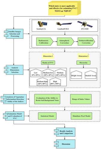
The workflow for this study (Figure 2) shows the structural framework of the differences comparison in applicability and effectiveness of NSVI and NDVI for estimating FVC based on multi-source remote sensing images.

Figure 2. Workflow of the comprehensive comparison of the capability differences to detect vegetation information and FVC.

3. Results

3.1. Evaluation of the ability to resist soil background noise

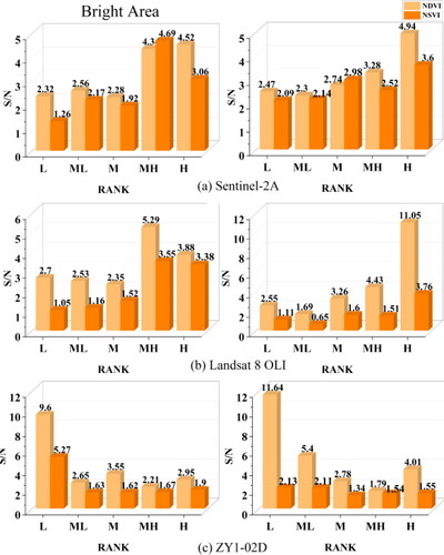
The signal-to-noise ratios (SNR) of all sample points in these three image data sources based on NSVI and NDVI indices at different hierarchies and different FVC ranks were calculated in Figure 3. The results showed that, in general, the SNR of NSVI is slightly smaller than that of NDVI in bright and shaded areas of the three image data sources, and the SNR of the two indices do not differ significantly in bright or shaded areas. Specifically, in bright areas of Sentinel-2A, the SNR of NSVI is smaller than that of NDVI except for the medium-high-rank FVC areas, and the maximum difference is 1.46 in high-rank FVC areas, while in shaded areas, the SNR of NSVI is smaller than that of NDVI except for the medium-rank FVC areas, and the maximum difference is 1.94 in high-rank FVC areas. In bright and shaded areas of Landsat-8 OLI, the SNR of NSVI is smaller than NDVI in all ranks of FVC areas, and the maximum difference is 1.74 in bright areas and 7.29 in shaded areas in medium-high-rank of FVC areas. In bright and shaded areas of ZY1-02D, the SNR of NSVI is smaller than that of NDVI in all ranks of FVC areas, and the maximum difference in bright areas is 4.33 in low-rank FVC areas, and the maximum difference in shaded areas is 9.51 in low-rank FVC areas. The above showed that the overall ability of NSVI to resist the soil background is slightly inferior to that of NDVI, and the ability of both to eliminate the soil background is not significantly affected by ‘bright’ and ‘shadow’ hierarchies.

Figure 3. Comparison results of indices SNR for each rank. L, ML, M, MH and H represent low-rank FVC, medium-low-rank FVC, medium-rank FVC, medium-high-rank FVC and high-rank FVC, respectively.

3.2. Evaluation of the impact of the range of index values on vegetation information detection

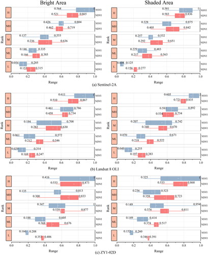
The range of values of NSVI and NDVI at each FVC rank in ‘bright’ and ‘shadow’ hierarchies of the three image data sources were summarized statistically. The difference between the maximum and minimum values of vegetation indices is shown in Figure 4. The results showed that, in general, the ranges of both indices showed a fluctuating trend of increasing and then decreasing as the FVC rank increases, and the ranges of both indices do not show significant differences in bright or shaded areas; specifically, in bright areas of Sentinel-2A, the range of NSVI is larger than NDVI except for the medium-low-rank FVC areas, and the largest difference was found in medium-high-rank FVC areas, with a difference of 12.1%; in shaded areas, the range of NSVI is smaller than NDVI except for the medium-high-rank FVC areas, and the largest difference was found in medium-high-rank FVC areas, with a difference of 12.1%. In bright and shaded areas of Landsat-8 OLI, the range of NSVI was larger than NDVI in all ranks of FVC, and the maximum difference of the bright areas was 17.6% in medium-high-rank FVC areas, and the maximum difference of the shaded areas was 29.7% in medium-high-rank FVC areas. In bright areas of ZY1-02D, the range of NSVI was larger than NDVI except for the low-rank FVC areas, and the maximum difference was found in medium-high-rank FVC areas, with a difference of 31.4%; in shaded areas, the range of NSVI was larger than NDVI except for the medium-high-rank FVC areas, and the maximum difference was found in medium-high-rank FVC areas, with a difference of 36.8%. In summary, the difference in the range of NSVI and NDVI indices reflects that their ability to detect vegetation information is not significantly influenced by ‘bright’ and ‘shadow’ hierarchies and NSVI is slightly better than NDVI in detecting vegetation information in aggregate, especially in areas with medium-high-rank and high-rank FVC areas.

Figure 4. Comparison of the index range. Blue and red boxes are the range of NSVI and NDVI, respectively, the range of NSVI is slightly larger than NDVI in aggregate, and the range of both values are not significantly affected by the bright and shadow hierarchies.

3.3. Sensitivity analysis of FVC

The true values of FVC of all sample sites in this study were correlated with their corresponding NSVI and NDVI index values in Table 4. The results showed that NSVI, NDVI and FVC presented highly significant correlations in different hierarchies of ‘bright’ and ‘shadow’ in three image data sources, without differentiating the ranks. In terms of correlation coefficients, the correlation between NSVI and FVC is slightly more significant compared to the NDVI. Combining different hierarchies with different FVC ranks, in general, the correlation between NSVI and FVC is slightly more significant than NDVI in low-rank, medium-low-rank, medium-high-rank, and high-rank FVC areas and slightly less significant than NDVI in shaded areas. Specifically, in Sentinel-2A, the correlation between NSVI and FVC was highly significant (p < 0.01) except for the medium-rank FVC areas in bright areas and the medium-rank FVC areas in shaded areas, and significant (p < 0.05) in low-rank and medium-rank in shaded areas; the correlation between NDVI and FVC was highly significant (p < 0.01) in low-rank and high-rank FVC areas in bright areas and the medium-rank FVC areas of the shaded areas (p < 0.05). In Landsat-8 OLI, the correlation between NSVI and FVC was highly significant (p < 0.01) for all ranks of FVC areas in bright areas and low-rank and high-rank FVC areas in shaded areas, and significant (p < 0.05) for low-rank and medium-high-rank FVC areas in shaded areas.; the correlation between NDVI and FVC was highly significant (p < 0.01) in medium-high-rank and high-rank FVC areas in bright areas and in low-rank, medium-low-rank and high-rank FVC areas in shaded areas, and significant (p < 0.05) in low-rank FVC areas in bright areas. In ZY1-02D, the correlation between NSVI and FVC was highly significant (p < 0.01) in medium-rank FVC areas in shaded areas and significant (p < 0.05) in high-rank FVC areas in shaded areas; the correlation between NDVI and FVC was highly significant (p < 0.01) in low-rank FVC areas in shaded areas and significant (p < 0.05) in medium-rank FVC areas in shaded areas. In summary, the correlation between NSVI, NDVI and FVC is significantly influenced by ‘bright’ and ‘shadow’ hierarchies and the correlation between NSVI and FVC is slightly more significant than NDVI in bright areas and slightly less significant than NDVI in shaded areas.

Table 4. Correlation of indices with FVC.

Satellite image			Sentinel-2A		Landsat-8 OLI		ZY1-02D
FVC Rank	Hierarchy	Statistical indicator	NDVI	NSVI	NDVI	NSVI	NDVI	NSVI
Low	Bright	ρ	0.747**	0.681**	0.508*	0.845**	0.771	0.429
	Shaded	ρ	0.700	0.700	0.817**	0.833**	0.943**	0.543
Medium-Low	Bright	ρ	0.405*	0.730**	0.118	0.560**	0.220	0.090
	Shaded	ρ	0.784**	0.749*	0.723**	0.588*	0.072	0.433
Medium	Bright	ρ	0.017	0.046	0.402	0.847**	0.483	0.469
	Shaded	ρ	0.478*	0.657**	0.404	0.181	0.510*	0.644**
Medium-high	Bright	ρ	0.313	0.492**	0.608**	0.687**	−0.055	0.064
	Shaded	ρ	0.442	0.374	0.161	0.655*	0.800	0.800
High	Bright	ρ	0.346*	0.470**	0.763**	0.743**	0.331*	0.178
	Shaded	ρ	0.371	0.654	0.670**	0.859**	0.155	0.285*
All ranks	Bright	ρ	0.930**	0.950**	0.920**	0.944**	0.705**	0.776**
	Shaded	ρ	0.903**	0.937**	0.941**	0.893**	0.823**	0.778**

Note: * indicates p < 0.05, significant correlation; ** indicates p < 0.01, highly significant correlation.

3.4. Estimation accuracy of statistical models

FVC true values of all samples in the three data sources and their corresponding NSVI and NDVI index values were respectively subjected to linear, quadratic, cubic, exponential, logarithm, power univariate fitting and multivariate fitting, and the optimal estimation model are shown in Tables 5, 6 and 7. The results showed that, overall, all FVC estimation models passed the confidence test of p < 0.01, and in terms of the goodness of fit, R² > 0.75 in Sentinel-2A and Landsat-8 OLI except for the exponential model; R² > 0.5 in ZY1-02D for all models. In terms of the preferred model perspective in Figures 5, 6 and 7, the best-fit FVC models for both indices in bright and shadow hierarchies in Sentinel-2A and Landsat-8 OLI are all cubic models, and the best-fit FVC models for both indices in bright areas in ZY1-02D are power models, and in shaded areas are cubic models; in terms of different hierarchies, the ‘bright’ and ‘shadow’ hierarchies of the same regression model have a significant effect on the goodness of fit, and the goodness of fit in bright areas is slightly higher than that in shaded areas. In Sentinel-2A, the fit of the NSVI-based estimation model is slightly better than that of NDVI in both bright and shadow hierarchies. The optimal univariate estimation equations based on each index are shown in Table 5.

Figure 5. Regression functions between FVC with NDVI and NSVI from Sentinel-2A.

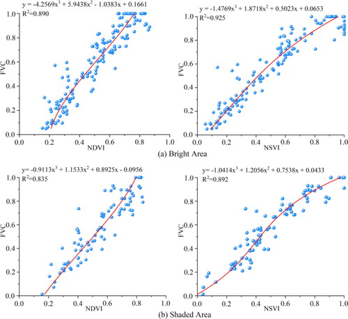
Figure 6. Regression functions between FVC with NDVI and NSVI from Landsat-8 OLI.

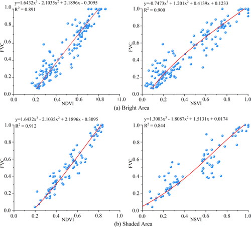
Figure 7. Regression functions between FVC with NDVI and NSVI from ZY1-02D.

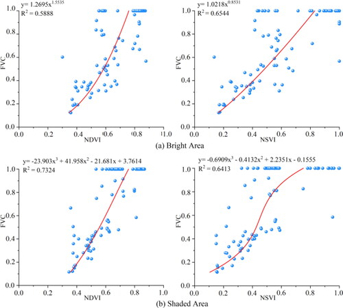
Table 5. Fitting relationship between indices and FVC.

Satellite image	Hierarchy	Optimal regression equation
		NDVI	NSVI
Sentinel-2A	Bright	y = −4.2569 × 3+5.9438 × 2−1.0383x + 0.1661	y = −1.4769 × 3+1.8718 × 2+0.5023x + 0.0653
	Shaded	y = −0.9113 × 3+1.1533 × 2+0.8925x − 0.0956	y = −1.0414 × 3+1.2056 × 2+0.7538x + 0.0433
Landsat-8 OLI	Bright	y = −1.7606 × 3+3.1266 × 2−0.2844x + 0.0858	y = −0.7473 × 3+1.201 × 2+0.4139x + 0.1233
	Shaded	y = 1.6432 × 3−2.1035 × 2+2.1896x − 0.3095	y = 1.3083 × 3−1.8087 × 2+1.5131x + 0.0174
ZY1-02D	Bright	y = 1.2695 × 1.5535	y = 1.0218 × 0.8531
	Shaded	y = −23.903 × 3+41.958 × 2−21.681x + 3.7614	y = −0.6909 × 3−0.4132 × 2+2.2351x − 0.1555

Table 6. FVC univariate regression statistics.

Satellite image			Sentinel-2A		Landsat-8 OLI		ZY1-02D
Model	Hierarchy	Statistical indicator	NDVI	NSVI	NDVI	NSVI	NDVI	NSVI
Primary linear model	Bright	R^2	0.876**	0.894**	0.887**	0.898**	0.547**	0.618**
	Shaded	R^2	0.833**	0.874**	0.908**	0.829**	0.699**	0.530**
Quadratic linear model	Bright	R^2	0.882**	0.919**	0.888**	0.898**	0.553**	0.638**
	Shaded	R^2	0.834**	0.886**	0.911**	0.837**	0.728**	0.641**
Cubic linear model	Bright	R^2	0.890**	0.925**	0.889**	0.901**	0.553**	0.638**
	Shaded	R^2	0.835**	0.892**	0.912**	0.844**	0.732**	0.641**
Power model	Bright	R^2	0.861**	0.873**	0.846**	0.786**	0.550**	0.625**
	Shaded	R^2	0.809**	0.758**	0.861**	0.719**	0.717**	0.612**
Logarithmic model	Bright	R^2	0.829**	0.881**	0.835**	0.798**	0.589**	0.654**
	Shaded	R^2	0.813**	0.871**	0.868**	0.802**	0.717**	0.632**
exponential model	Shaded	R^2	0.763**	0.750**	0.804**	0.783**	0.563**	0.592**
	Shaded	R^2	0.721**	0.709**	0.807**	0.744**	0.677**	0.507**

Note: * indicates p < 0.05, significant correlation, and the regression relationship between the variables is significant; ** indicates p < 0.01, highly significant correlation, and the regression relationship between the variables is highly significant.

Table 7. FVC multivariate regression statistics.

Satellite image			Sentinel-2A	Landsat-8 OLI	ZY1-02D
Model	Hierarchy	Statistical indicator	NDVI-NSVI
Multivariate linear	Bright	R^2	0.909**	0.910**	0.619**
	Shaded	R^2	0.889**	0.910**	0.726**

Note: * indicates p < 0.05, significant correlation, and the regression relationship between the variables is significant; ** indicates p < 0.01, highly significant correlation, and the regression relationship between the variables is highly significant.

In summary, the statistical models constructed by NSVI and NDVI can meet the effective estimation of FVC with high accuracy, and the accuracy of the estimation models of NSVI, NDVI and FVC is influenced by ‘bright’ and ‘shadow’ hierarchies. The accuracy of the estimation models of NSVI, NDVI and FVC was influenced by ‘bright’ and ‘shadow’ hierarchies, the goodness of fit in bright areas is slightly higher than that in shaded areas. Compared with NDVI, the goodness of fit of the five univariate regression models obtained by NSVI showed more significant strengths in bright areas.

3.5. Estimation accuracy of dimidiate pixel model

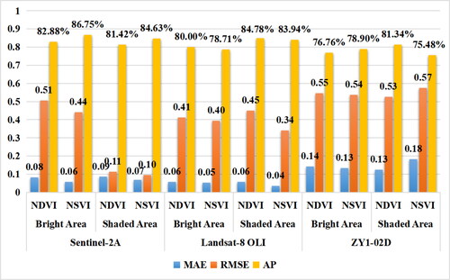
The calculation accuracy and errors of the FVC of the two indices for all sample sites in this study were summarized in Figure 8. The results showed that, without distinguishing FVC ranks, in terms of the volatility of the estimated data, the MAE and RMSE of FVC estimated based on NSVI were slightly smaller than those of NDVI among the three image data sources in general; the stability of the estimation in bright areas was slightly better than that in shaded areas. In terms of estimation accuracy, for different hierarchies of the same index, the estimation accuracy based on NDVI is slightly higher in bright areas in Sentinel-2A, the estimation accuracy based on NSVI is slightly higher in bright areas in Sentinel-2A and ZY1-02D, while in other areas, the estimation accuracy in shaded areas is slightly higher; for the same hierarchy of different indices, the estimation accuracy based on NSVI is slightly higher than NDVI in Sentinel-2A and ZY1-02D, while it is slightly lower than NDVI in Landsat-8 OLI.

Figure 8. Comparison of FVC estimation effects. The FVC estimates of the three images are better in bright areas than in shaded areas, and NSVI-based FVC estimation is more stable.

Combined with the different hierarchies of ‘bright’ and ‘shadow’ and different FVC ranks in Figure 9, the estimation accuracy was evaluated as follows, the estimation accuracy of NSVI and NDVI is the highest in high-rank FVC areas of Sentinel-2A and Landsat-8 OLI multispectral images, and the trend increases with the increase of FVC rank, while the trend is not obviously observed in ZY1-02D. Specifically, in bright areas of Sentinel-2A, the accuracy of NSVI-based estimation is slightly higher than NDVI in low-rank, medium-rank, medium-high-rank, high-rank FVC areas and slightly lower than NDVI in low-rank FVC areas; in shaded areas, the difference between the accuracy of NSVI and NDVI estimation is the same as that in bright areas. in bright areas of Landsat-8 OLI, the estimation accuracy based on NSVI is slightly higher than NDVI in medium-rank, medium-high-rank and high-rank FVC areas, and slightly lower than NDVI in low-rank, medium-low-rank FVC areas; in shaded areas, the estimation accuracy based on NSVI is slightly higher than NDVI in medium-low-rank and medium-high-rank FVC areas, and slightly lower than NDVI in low-rank, medium-rank and high-rank FVC areas. The difference between the estimation accuracy of NSVI and NDVI is slightly smaller. In bright areas of ZY1-02D, the estimation accuracy based on NSVI is slightly higher than NDVI in medium-low-rank, medium-high-rank and high-rank FVC areas, and slightly lower than NDVI in low-rank and medium-low-rank FVC areas; in shaded areas, the estimation accuracy based on NSVI is slightly higher than NDVI in low-rank, medium-rank FVC areas, and slightly lower than NDVI in low-rank, medium-high-rank and high-rank FVC areas.

Figure 9. Comparison results of FVC estimation accuracy for each rank.

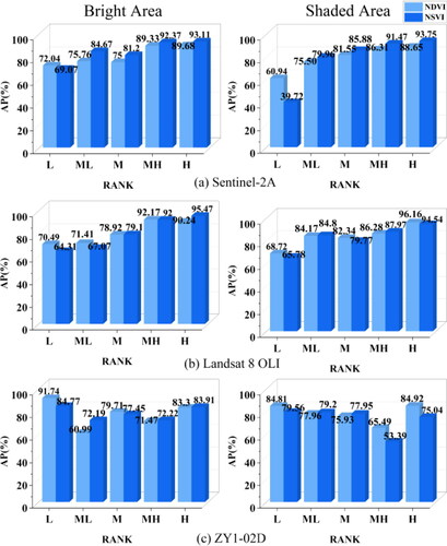
In summary, the estimation accuracy of the dimidiate pixel model that is based on NSVI and NDVI in this study is obviously affected by ‘bright’ and ‘shadow’ hierarchies; the accuracy of estimated FVC based on NSVI is slightly higher than that of NDVI in medium-high-rank and high-rank areas in bright areas and the error is more stable; the difference of estimation accuracy between the two indices is relatively small.

4. Discussion

4.1. Differences in vegetation information in bright and shaded areas

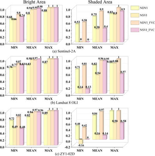
It can be found that there are obvious differences in the FVC estimation results under the influence of ‘bright’ and ‘shadow’ hierarchies, and it is easy to conclude that the vegetation information has obvious differences in bright and shaded areas as well. In order to investigate whether the difference has more manifestation or chance, this study reselected a certain number of bright and shaded vegetation pixels, obtained their spectral curves, maximum, minimum and mean values and plotted them as shown in Figures 10 and 11. It can be found that: (1) The vegetation spectral curves of ‘bright’ and ‘shaded’ areas in different data sources have obvious differentiability; (2) the vegetation spectra in shaded areas still have the information of ‘green peaks and red valleys’, but the feature is slightly ‘weakened’ compared with the bright areas; (3) the index values of NSVI, NDVI and FVC are similar. NDVI and FVC values showed a decreasing trend from bright areas to shaded areas, and the magnitude and degree of change of NSVI are greater than those of NDVI, which indicates that NSVI is more sensitive to the detection of shaded areas to some extent.

Figure 10. Vegetation curves in bright and shaded areas. Among the three image data sources, the vegetation reflectance curves in bright areas are higher than those in shaded areas and the differences are more obvious, but they show an overall consistent trend between different bands.

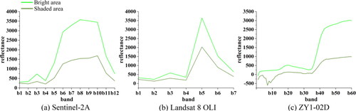
Figure 11. Comparison of vegetation information in bright and shaded areas.

4.2. Effect of ‘high’ and ‘low’ brightness shaded areas on FVC estimation

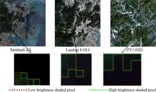
During the detection of vegetation information in shaded areas of the above three data sources, a bit differences were found in the variations of the two indices and their corresponding FVC and when the images were further visually interpreted, it was found that vegetation areas with obvious high and low brightness differences existed in various data sources in Figure 12. Therefore, it needs to be explored further, and the steps are as follows: initially, based on the visual interpretation results, about 300 randomly selected pixels in high and low brightness shaded vegetation areas of the three data sources are used as samples for statistics, and the NSVI and NDVI index values and FVC of the corresponding pixels of each data source sample are obtained respectively.

Figure 12. Diagrammatic sketch of ‘high and low brightness’ shaded areas. The examples in three image data sources showed the obvious difference in brightness between the high and low brightness shaded areas, with the brown outline areas being the vegetation pixels in low brightness shaded areas and the green outline areas being the vegetation pixels in high brightness shaded areas.

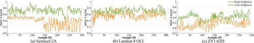
Division of ‘high and low brightness shaded areas’ threshold. The variation curves of NSVI and NDVI for the corresponding areas of each data source were plotted in Figures 13 and 14, and according to the variation curves, it can be seen that NDVI has an obvious range of high and low brightness shaded areas in Sentinel-2A image, but it is difficult to be divided in Landsat-8 OLI and ZY1-02D images; thus, NSVI has superior separability in Sentinel-2A and Landsat-8 OLI image data. Therefore, NSVI = 0.6 can be used as the threshold for dividing high and low brightness shaded areas in Sentinel-2A and Landsat-8 OLI data, and NSVI = 0.4 can be used as the threshold for dividing high and low brightness shaded areas in ZY1-02D data, that is, areas above 0.6 and 0.4 are high brightness shaded areas of multispectral and hyperspectral images, respectively, and areas below 0.6 and 0.4 are low brightness shaded areas of multispectral and hyperspectral images, respectively.

Figure 13. NDVI index variation curves in different brightness shaded areas. NDVI does not show significant differences in high or low brightness shaded areas of the three image data sources, and its differentiability is slightly weak, indicating that its ability to detect vegetation information in different brightness shaded areas is slightly weak.

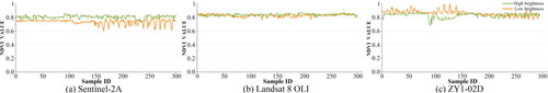
Figure 14. NSVI index variation curves in different brightness shaded areas. NSVI showed significant differences in high and low brightness shaded areas of the three image data sources, with slightly stronger differentiability, indicating slightly stronger sensitivity and ability to detect vegetation information in different brightness shaded areas.

The differences in vegetation information in ‘high and low brightness shaded areas’ and their effects on the FVC estimated values were further explored. The mean square deviation of NSVI, NDVI and their corresponding FVC estimated values for all pixels were plotted in Figures 15 and 16. In low brightness shaded areas of Sentinel-2A and Landsat-8 OLI, the difference of mean square between the NSVI and NDVI index values and their corresponding FVC estimates is slightly larger than that in high brightness shaded areas, while the NSVI and NDVI index values in high and low brightness shaded areas in the ZY1-02D data are consistent with the other two multispectral data, but FVC corresponding to the two indices is opposite to the other two data. The above results showed that the dispersion of background noise, index value and FVC in high brightness shaded areas is slightly smaller than that in low brightness shaded areas. To further verify the rationality of this law, the estimation accuracy of the shaded areas in the original sample of this study is divided and statistically plotted according to the above threshold, and it is easy to see that the estimation accuracy of FVC in high brightness shaded areas is significantly superior to that in low brightness shaded areas.

Figure 15. Differences in vegetation information and estimation effects of indices in shaded areas of different brightness. (a) Showed the standard deviation of shaded areas with different brightness; (b) Showed the comparison of FVC estimation accuracy in different brightness shaded areas.

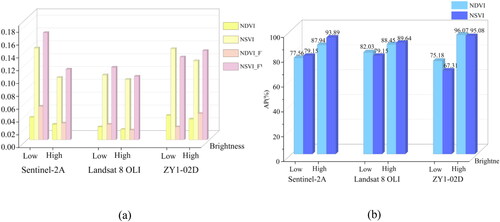
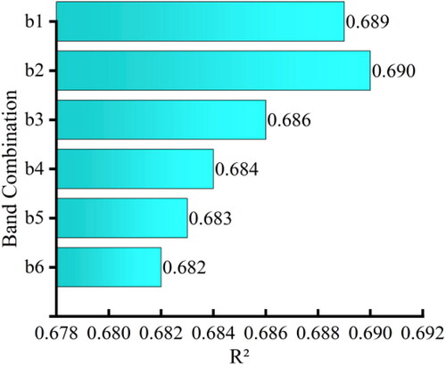
Figure 16. Comparison of the accuracy of the optimal regression model with different band combinations. b1–b7 band combinations are 680–800 nm, 680–808 nm, 680–825 nm, 680–834 nm, 680–843 nm and 680–860 nm, respectively, among which 680–808 nm is the most accurate band combination reflecting the vegetation cover information.

In summary, for the ‘high and low brightness shaded areas’, the NSVI-based classification is more effective, and the FVC estimation effect and accuracy are more stable and superior in ‘high brightness shaded areas’. The obvious difference between high and low brightness shaded areas may be the direct cause of the difference in FVC estimation in shaded areas of different image data sources.

4.3. Optimal band combination selection for hyperspectral vegetation information

In this study, multiple data sources were used to investigate the capability and generalizability of NSVI and NDVI in estimating FVC, but when constructed the FVC statistical model and dimidiate pixel model based on the hyperspectral data ZY1-02D, it was found that the model was slightly less stable and less accurate than the other two multispectral data sources. This may be due to the fact that the shaded areas present a big obstruction in information recognition and target detection in hyperspectral image, and there is difficulty in decomposing the shadow mixed pixels of hyperspectral image using a linear model (Roper and Andrews 2013; Oduncu and Yuksel 2021). It is also possible that during the construction of the ZY1-02D vegetation index, the NIR band and red band were selected according to the band combinations commonly used by related scholars, that is, the NIR band was selected with a central wavelength close to 800 nm, and the red band was selected with a central wavelength close to 680 nm, but the range of red band in ZY1-02D covers 20 bands from 620 to 780 nm, and the NIR band range covers 60 bands from 780 to 1500 nm. If the vegetation index is constructed and the invalid band information is excluded, there are 1120 band combinations. However, whether the band combination selected in this study is the optimal combination to respond to the vegetation information needs further research to prove (Li et al. 2010; Kim et al. 2014), and the steps are as follows:

1. Extract NSVI and NDVI index values and their corresponding FVC values under 1120 band combinations.

2. Exclude the effect of covariance by the Spearman correlation analysis method with a superior ability, a total of six band combinations with the highest correlation with the true value of FVC were identified, namely: 680–800 nm, 680–808 nm, 680–825 nm, 680–834 nm, 680–843 nm, 680–860 nm.

3. Construct the best statistical model using the six band combinations into an index with the true value of FVC and compare their model superiority in Figure 16.

After the optimal band selection, it is easy to find that the optimal regression models constructed by the six band combinations are all power models, and the R² accuracy of the model under the 680–808 nm band combination is the highest at 0.69 and slightly higher than that of the band combination selected in this article, so the band selection in hyperspectral data does affect the estimation effect of FVC, but the selected band combination in this article is only second to the optimal band combination and the difference in accuracy is very small, which is essential to the study of FVC estimation of hyperspectral data.

4.4. Inversion results of FVC

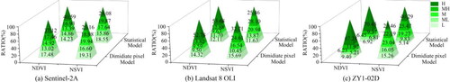
From the perspective of inversion results in Figures 17, 18, 19 and 20, it is easy to find that under the different FVC estimation models of the three image data sources, the differences between NSVI and NDVI are most obvious in high-rank FVC areas, and the MINUS values are clustered in the range of −0.25 to 0.25 and their proportion is more than 85%, among which the highest proportion is in the range of 0–0.25. Above showed that the difference between FVC estimation based on NDVI and NSVI is slightly smaller in general; secondly, the FVC estimation of NDVI is higher than that of NSVI; finally, NDVI has the deficiency of oversaturation in high-rank FVC area (Guo et al. 2019; Zhao et al. 2020).

Figure 17. Thematic chart of Sentinel-2A inversion results. The difference value is the FVC estimated based on NDVI minus the FVC estimated based on NSVI for each pixel, the same below. Differences in results of inversion are most obvious in high-rank FVC areas.

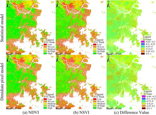
Figure 18. Thematic chart of Landsat 8 OLI inversion results. Differences in results of inversion are most obvious in high-rank FVC areas.

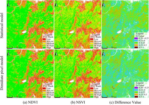
Figure 19. Thematic chart of ZY1-02D inversion results. Differences in results of inversion are most obvious in high-rank FVC areas.

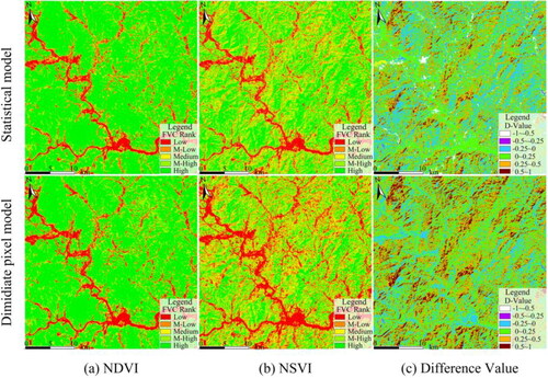
Figure 20. Inversion results of test area ratio of FVC for each rank.

4.5. Potential of applying NSVI to estimate FVC and prospects

From the above study, it can be found that the FVC estimation ability of NSVI has obvious advantages in medium-high-rank and high-rank FVC areas, but at the same time, NSVI also has some deficiencies in the ability to eliminate soil background, and the advantages are not obvious in low-rank FVC areas, which is because NSVI was initially constructed for mountainous and hilly areas, that is, for areas with high-rank FVC areas, without considering non-forested areas such as partly buildings, impervious surface and so on, which were treated with mask removal. To improve the overall estimation ability of NSVI on FVC, the idea of improving this index can be based on the construction principle of Soil-Adjusted Vegetation Index SAVI (Eq. 10(10) $$\text{RMSE}=\sqrt{\frac{\sum _{i=1}^n{\left(\text{FVC}-\text{FVC}\prime \right)}^2}{n}}$$(10) ). Huete et al. and Bausch et al. pointed out in their research on the construction and application of SAVI that the introduction of scientific and reasonable soil-adjusted factors can eliminate or mitigate the effects of soil background (Huete 1988; Bausch 1993). However, any vegetation index has its application range and certain defects. The SAVI index with the function of reducing soil noise performs better in low-rank and medium-rank FVC areas, but it is also affected by the soil-adjusted factor L, which makes the vegetation information of its shaded slopes weaker than that of bare soil, thus reducing the ability of SAVI to detect the vegetation information of shaded slopes and generating the inaccuracy of vegetation information estimation (Li et al. 2015). Thus, the improvement of NSVI will try to apply a soil adjustment factor in the subsequent stage of the study, and pay more attention to improving the ability of this index to eliminate soil background while ensuring the existing advantages and learning from the defects of SAVI index, so as to improve the overall vegetation information detection ability of the index.

5. Conclusions

1. The ability of NDVI to resist soil background noise is slightly greater than the one of NSVI for the three image data sources, and the SNR of the two indices do not differ significantly in bright or shaded areas.

2. From the perspective of index range, both indices showed a fluctuating upward trend with the increase of FVC rank and the range of both indices did not show significant differences in bright or shaded areas; the range of NSVI and NDVI is slightly larger compared to those of Sentinel-2A and Landsat-8 OLI in ZY1-02D; NSVI is slightly stronger than NDVI in detecting vegetation information in general, especially in medium-high-rank and high-rank FVC areas.

3. Without differentiating the rank, NSVI, NDVI and FVC showed highly significant correlations in bright and shaded areas of the three image data sources, and the correlation coefficients showed that the correlation between NSVI and FVC is slightly superior to that between NDVI and FVC. Combining the different hierarchies with the different FVC ranks, the correlation between NSVI and FVC is slightly more significant than NDVI in low-rank, medium-low-rank, medium-high-rank and high-rank FVC areas in bright areas, and slightly less significant than NDVI in shaded areas. From the perspective of the constructed FVC statistical model, the effective estimation of FVC can be satisfied by NSVI or NDVI with high accuracy, furthermore, the accuracy of the estimation model of NSVI, NDVI and FVC is influenced by ‘bright’ and ‘shadow’ hierarchies obviously. In comparison, the bright and shadow hierarchies of the same regression model have a significant effect on the goodness of fit, that is, the goodness of fit in bright areas is slightly higher than that in shaded areas; compared with NDVI, the goodness of fit of the five binary regression models obtained by NSVI showed a significant advantage in bright areas, among which the best fit is obtained by the cubic curve model.

4. The estimation accuracy of the dimidiate pixel model based on NSVI and NDVI is obviously affected by ‘bright’ and ‘shadow’ hierarchies; the estimation accuracy of FVC based on NSVI is slightly higher than that of NDVI in medium-high-rank and high-rank FVC areas in bright areas, and the error is more stable; the difference of estimation accuracies is relatively small.

5. Shaded areas with different levels of brightness exist in different image data sources and can lead to significant errors in the FVC estimation results. Compared to NDVI, NSVI-based thresholding can effectively distinguish shaded areas of different brightness and the FVC estimation is more stable and better in ‘high-brightness shaded areas’.

Summarizing the above among the statistical model and the dimidiate pixel model, the FVC estimation ability of NSVI and NDVI is influenced by the different hierarchies of ‘bright’ and ‘shadow’, and the estimation effect of NSVI and NDVI is slightly better in bright areas than in shaded areas. By comparison, the accuracy of estimated FVC based on NSVI is slightly higher than that of NDVI in medium-high-rank and high-rank FVC areas in bright areas, both of them have their respective advantages in eliminating soil background and detecting vegetation information. The NSVI is preferred in areas with medium-high-rank and high-rank FVC, while the NDVI is preferred in areas with low-rank FVC in shaded areas.

Authors’ contributions

Conceptualisation, Z.X. and Y.L.; methodology and software, Z.X. and Y.L.; data collection and process, Y.L., B.L., X.Z., H.Y. and S.X.; validation and modification, Z.H., L.L., X.H., P.L., W.S., A.H., L.C. and Z.L.; writing—original draft preparation, Y.L.; writing—review and editing, Z.X. and Y.L.; project administration, Z.X.; funding acquisition, Z.X. All authors have read and agreed to the published version of the manuscript.

Acknowledgements

The authors would like to thank the anonymous reviewers for their tremendous time, helpful suggestions, and insightful comments, which greatly improved our manuscript.

Disclosure statement

No potential conflict of interest was reported by the authors.

Data availability statement

Data and associated codes are available from the corresponding author upon reasonable re-quest.

Additional information

Funding

This research was funded by the National Natural Science Foundation of China, Grant Number 42071300; by the Fujian Province Natural Science Foundation Project, Grant Number 2020J01504; by the China Postdoctoral Science Foundation, Grant Number 2018M630728; by the Open Fund of Fujian Provincial Key Laboratory of Resources and Environment Monitoring & Sustainable Management and Utilization, Grant Number ZD202102; by the Open Fund of University Key Lab of Geomatics Technology and Optimize Resources Utilization in Fujian Province, Grant Number fafugeo201901; and Supported by the Research Project of Jinjiang Fuda Science and Education Park Development Center, Grant Number 2019-JJFDKY-17 (Corresponding author: Zhanghua Xu.).

References

- Andrew DR, Trevor FK, Mirco M, Youngryel R, Oliver S, Michael T. 2013. Climate change, phenology, and phenological control of vegetation feedbacks to the climate system. Agric For Meteorol. 169(3):156–173.
- Arekhi M, Goksel C, Sanli FB, Senel G. 2019. Comparative evaluation of the spectral and spatial consistency of sentinel-2 and Landsat 8 OLI Data for Igneada Longos Forest. IJGI. 8(2):56.
- Badgley G, Field CB, Berry JA. 2017. Canopy near-infrared reflectance and terrestrial photosynthesis. Sci Adv. 3(3).
- Barsi JA, Alhammoud B, Czapla-Myers J, Gascon F, Haque MO, Kaewmanee M, Leigh L, Markham BL. 2018. Sentinel-2A MSI and Landsat 8 OLI radiometric cross comparison over desert sites. Eur J Remote Sens. 51(1):822–837.
- Bausch WC. 1993. Soil background effects on reflectancebased crop coefficients for corn. Remote Sens Environ. 46(2):213–222.
- Carlson TN, Gillies RR, Perry EM. 1994. A method to make use of thermal infrared temperature and NDVI measurements to infer surface soil water content and fractional vegetation cover. Remote Sens. Rev. 9(1-2):161–173.
- Chastain R, Housman I, Goldstein J, Finco M, Tenneson K. 2019. Empirical cross sensor comparison of sentinel-2A and 2B MSI, Landsat 8 OLI, and Landsat 7 ETM + top of atmosphere spectral characteristics over the conterminous United States. Remote Sens Environ. 221:274–285.
- Chen YX, Qin K, Hu ZW, Zeng C. 2019. A method of representing and merging and extracting building blocks from high-resolution images. Geomatics Inf. Sci. Wuhan Univ. 44(6):908–916.
- Crowther TW, Glick HB, Covey KR, Bettigole C, Maynard DS, Thomas SM, Smith JR, Hintler G, Duguid MC, Amatulli G, et al. 2015. Mapping tree density at a global scale. Nature. 525(7568):201–205.
- Cui TX, Gong ZN, Zhao WJ, Zhao YL, Lin C. 2013. Research on estimating wetland vegetation abundance based on spectral mixture analysis with different endmember model: a case study in Wild Duck Lake wetland, Beijing Acta Ecol Sin. 33(4):1160–1171.
- Dong SG, Qin JX, Guo YK. 2019. Shadow detection method for high-resolution remote sensing images supported by generalized stereoscopic image pair. J El Me In. 33(3):105–111.
- Gitelson AA, Kaufman YJ, Stark R, Rundquist D. 2002. Novel algorithms for remote estimation of vegetation fraction. Remote Sens Environ. 80(1):76–87.
- Guerschman JP, Hill MJ, Leys J, Heidenreich S. 2020. Vegetation cover dependence on accumulated antecedent precipitation in Australia: relationships with photosynthetic and non-photosynthetic vegetation fractions. Remote Sens Environ. 240:111670.
- Gunasekara NK, Al-Wardy MM, Al-Rawas GA, Charabi Y. 2015. Applicability of VI in arid vegetation delineation using shadow-affected SPOT imagery. Environ Monit Assess. 187(7):4662.
- Guo ZW, Wu CY, Wang XY. 2019. Forest insect-disease monitoring and estimation based on satellite remote sensing data. Geogr Res. 8(4):831–843.
- Guzinski R, Nieto H. 2019. Evaluating the feasibility of using Sentinel-2 and Sentinel-3 satellites for high-resolution evapotranspiration estimations. Remote Sens Environ. 221:157–172.
- Hansen M, Potapov P, Margono B, et al. 2014. High-resolution global maps of 21st-century forest cover change. Science. 342(6187):850–853.
- Hirano Y, Yasuoka Y, Ichinose T. 2004. Urban climate simulation by incorporating satellite-derived vegetation cover distribution into a mesoscale –meteorological model. Theor Appl Climatol. 79(3-4):175–184.
- Hu XY, Xu ZH, Chen WH, Chen QX, Wang L, Liu H, Liu ZC. 2021. Construction and application effect of normalized shaded vegetation index NSVI based on PROBA/CHRIS image. Remote Sens Land Resour. 33(2):55–65.
- Huete AR. 1988. A soil-adjusted vegetation index (SAVI). Remote Sens Environ. 25(3):295–309.
- Huete A, Didan K, Miura T, Rodriguez EP, Gao X, Ferreira L. 2002. Overview of the radiometric and biophysical performance of the MODIS vegetation indices. Remote Sens Environ. 83(1/2):195–213.
- Jiang H, Yuan YW, Wang S. 2019. Shadow-eliminated vegetation index (SEVI) for removing terrain shadow effect: evaluation and application. J Geoinf Sci. 21(12):1977–1986.
- Jiao JN, Shi J, Tian QJ, Gao L, Xu NX. 2020. Research on multispectral-image-based NDVI shadow-effect eliminating model. J Remote Sens. 24(1):53–66.
- Kim TW, Wie GJ, Suh YC. 2014. An adequate band selection for vegetation index of CASI-1500 airborne hyperspectral imagery using image differencing and spectral derivative. J Korean Assoc Geogr Inf Stud. 6(4):16–28.
- Leprieur C, Kerr YH, Mastorchio S, Meunier JC. 2000. Monitoring vegetation cover across semi-arid regions: comparison of remote observations from various scales. Int J Remote Sens. 21(2):281–300.
- Li J, Guo YB, Xu HQ, Li X. 2015. Vegetation information extraction of Pinus Massoniana Forest in soil erosion areas using soil-adjusted vegetation index. J Geoinf Sci. 17(9):1128–1134.
- Li XS, Li ZY, Gao ZH, Bai LN, Wang BY, Li SM. 2010. Estimation of sparse vegetation cover in arid regions based on vegetation indices derived from Hyperion data. J Beijing For Univ. 32(3):95–100.
- Li XW, Shi H, Zhang Y, Niu ZC, Wang TT, Ding M, Cai K. 2018. Cyanobacteria blooms monitoring in Taihu Lake based on the Sentinel-2A satellite of European Space Agency. Environ Monit China. 34(4):169–176.
- Liu F, Liu SH, Xiang Y. 2014. Research on UAV remote sensing monitoring of vegetation cover in gardens. Trans Chin Soc Agric Mach. 45(11):250–257.
- Liu C, Zhang X, Wang T, Chen G, Zhu K, Wang Q, Wang J. 2022. Detection of vegetation coverage changes in the Yellow River Basin from 2003 to 2020. Ecol Indic. 138:108818.
- Liu XT, Zhou L, Shi H, Wang SQ, Chi YG. 2018. Phenological characteristics of temperate coniferous and broad-leaved mixed forests based on multiple remote sensing vegetation indices, chlorophyII fluorescence and CO2 flux data. Acta Ecol Sin. 38(10):3482–3494.
- Li CJ, Zhao CJ, Liu LY, Wang JH, Wang RC. 2004. Infrared spectral index inversion of field winter wheat cover and sensitivity analysis. Trans CSAE. 20(5):159–164.
- Li MX, Zhu XC, Bai XY, Peng YF, Tian ZY, Jiang YM. 2021. Remote sensing inversion of nitrogen content in apple canopy based on shadow removal in UAV multi-spectral remote sensing images. Sci Agric Sin. 54(10):2084–2094.
- Mancino G, Ferrara A, Padula A, Nolè A. 2020. Cross-comparison between Landsat 8(OLI)and Landsat 7(ETM+)Derived Vegetation Indices in a Mediterranean Environment. Remote Sens. 12(2):291.
- Oduncu E, Yuksel SE. 2021. An in-depth analysis of hyperspectral target detection with shadow compensation via LiDAR. Signal Process Image Commun. 99(4):116427.
- Ono A, Kajiwara K, Honda Y. 2010. Development of new vegetation indexes, shadows index (SI) and water stress trend (WST). N W Remote Sens. 38(1):710–714.
- Owen TW, Carlson TN, Gillies RR. 1998. An assessment of satellite remotely-sensed land cover parameters in quantitatively describing the climatic effect of urbanization. Int J Remote Sens. 19(9):1663–1681.
- Pudmenzky C, King R, Butler H. 2015. Broad scale mapping of vegetation cover across Australia from rainfall and temperature data. J Arid Environ. 120:55–62.
- Qi J, Chehbouni A, Huete AR, Kerr YH, Sorooshian S. 1994. A modified soil adjusted vegetation index. Remote Sens Environ. 48(2):119–126.
- Roper T, Andrews M. 2013. Shadow modelling and correction techniques in hyperspectral imaging. Electron Lett. 49(7):458–459.
- Rouse JW, Haas RH, Schell JA. 1973. Monitoring vegetation systems in the Great Plains with ERTS. The 3rd ERTS Symposium, NASA SP-351, vol. 1, p. 309–317.
- Rundquist BC. 2002. The influence of canopy green vegetation fraction on spectral measurements over native tallgrass prairie. Remote Sens Environ. 81(1):129–135.
- Shen JX, Ji X. 2016. Cloud and cloud shadow multi-feature collaborative detection from remote sensing image. J Geoinf Sci. 18(5):599–605.
- Silvoster ML, Govindan VK. 2012. Enhanced CNN based electron microscopy image segmentation. Cyb Inf Technol. 12(2):84–97.
- Song WJ, Mu XH, Ruan GY, Gao Z, Li LY, Yan GJ. 2017. Estimating fractional vegetation cover and the vegetation index of bare soil and highly dense vegetation with a physically based method. Int J Appl Earth Obs Geoinf. 58:168–176.
- Tian QJ, Min XJ. 1998. Advances in study on vegetation indices. Adv Earth Sci Contrib Int Conf. 13(4):10–16.
- Vupparaboina KK, Dansingani KK, Goud A, Rasheed MA, Jawed F, Jana S, Richhariya A, Freund KB, Chhablani J. 2018. Quantitative shadow compensated optical coherence tomography of choroidal vasculature. Sci Rep. 8(1):6461.
- Xu ZH, Lin L, Wang QF. 2018. Construction and application effects of normalized shaded vegetation index (NSVI). J Infrared Millim Waves. 37(2):154–162.
- Xu ZH, Liu J, Yu KY, Liu T, Gong CH, Tang MY, Xie WJ, Li ZL. 2013. Construction of Vegetation Shadow Index (SVI) and application effects in four remote sensing images. Spectrosc Spectral Anal (Beijing, China). 33(12):3359–3365.
- Yang QY, Jiang ZC, Luo WQ, Ma ZL, Cao JH, Shen LN. 2013. Sequential simulation of normal different vegetation index of mountain shadow in Karst Peak Cluster Area. Trans Chin Soc Agric Mach. 44(05):232–236.
- Zhang XX. 2016. A comparative study on different vegetation indices in capabilities for eliminating soil background noise and detecting vegetation coverage. Highlights Sciencepaper. 9(2):126–132.
- Zhang HM, Chen LJ, Liu W, Han WT, Zhang SY, Zhang F. 2021. Estimation of summer corn fractional vegetation coverage based on stacking ensemble learning. Trans Chin Soc Agric Mach. 52(7):195–202.
- Zhang LF, Sun XJ, Wu TX, Huang CP. 2015. An analysis of shadow effects on spectral vegetation indexes using a ground-based imaging spectrometer. IEEE Geosci Remote Sens Lett. 12(11):1–5.
- Zhao J, Yang HB, Lan YB, Lu LQ, Jia P, Li ZM. 2019. Extraction method of summer corn vegetation coverage based on visible light image of unmanned aerial vehicle. Trans Chin Soc Agric Mach. 50(5):232–240.
- Zhao LL, Zhang R, Liu YX, Zhu XC. 2020. The differences between extracting vegetation information from GF1-WFV and Landsat8-OLI. Acta Ecol Sin. 40(10):3495–3506.