Sentinel-2 mapping of a turbid intertidal seagrass meadow in Southern Vietnam

Abstract

Seagrass ecosystems are crucial to the carbon cycle, biodiversity, fisheries, and erosion prevention. However, there are gaps in mapping seagrass in tropical coastal waters due to turbidity and constantly changing tidal dynamics. To tackle such issues, tidal heights and reflectance of 33 Sentinel-2 images were used to calculate a multitemporal composite of Sentinel-2 images, which was classified using the Random Forest classifier. UAV images classified with Object-based image analysis provided ground truth for training and validation. The effectiveness of water column correction and using the multitemporal composite was evaluated by comparing overall classification accuracy. As a result, applying water column correction improved classification accuracy from 80.4% to 80.6%, while using the multi-temporal composite improved accuracy to 88.6%, among the highest accuracy achieved for seagrass classification in turbid waters. The combined protocol could lead to advances in quantifying seagrass distribution in the tropical coastal waters and their carbon sequestration capacity, resolving significant uncertainties in blue carbon estimation.

Keywords:

• blue carbon ecosystems
• seagrass mapping
• time series analysis
• object-based image analysis
• tidal dynamics
• unmanned aerial vehicles

View correction statement:

Correction

1. Introduction

The seagrass ecosystem is a component of the blue carbon ecosystems, which is a significant part of the global carbon cycle (Nellemann 2009; Duarte et al. 2010; McLeod et al. 2011; Fourqurean et al. 2012; Pendleton et al. 2012; Miyajima et al. 2015). Besides, seagrass ecosystems also play crucial roles in promoting biodiversity, supporting fisheries, and mitigating coastal erosion (Costanza et al. 1997; Gillanders 2007; Unsworth and Cullen 2010; de Groot et al. 2012; Cullen-Unsworth and Unsworth 2013; Costanza et al. 2014; Dewsbury et al. 2016; Unsworth et al. 2018). Despite those benefits, the distribution of seagrass ecosystems is undergoing rapid decline, with a global loss rate of 7% annually (Waycott et al. 2009) and a decline of 45–50% in Vietnam from the 1990s to the 2000s (Nguyen 2013) due to a combination of anthropogenic stress and climate change (’Waycott et al. 2009; Nguyen 2013; Vo et al. 2020). Thus, accurate mapping of seagrass ecosystems is crucial and urgently needed.

The estimation of seagrass distribution has seen significant improvement in recent years, driven by growing research interest in these ecosystems (Duarte 2002; Short 2004; McLeod et al. 2011; Hossain et al. 2015; Mitra and Zaman 2015; Phinn et al. 2018; Duffy et al. 2019; Sudo et al. 2021). Nevertheless, there still remain uncertainties in the estimation of global seagrass distribution, especially in the Tropical Pacific region (Unsworth et al. 2019; Sudo et al. 2021). Differently from the case of land cover mapping, in shallow water systems suspended sediments and dissolved organic matter affect the upwelling reflectance, which in turn impact the process of image classification. As a result, in 55 papers on seagrass mapping reviewed by (Pham et al. 2019), 78% overall accuracy is considered high for seagrass distribution mapping. Mapping seagrass beds on intertidal flats is particularly challenging due to the constantly changing surface reflectance (Murray et al. 2019), resulting in large uncertainties. This uncertainty negatively affects the estimation of seagrass condition and impedes further understanding of coastal ecosystems services.

To address the challenges of seagrass mapping in turbid waters, various approaches have been undertaken, including water column correction and data collection optimization. While water column correction techniques are typically optimised for clear water (Lyzenga 1978; 1981; Lee et al. 1999; Green et al. 2000; Matsunaga et al. 2000; Stumpf et al. 2003; Mumby et al. 2010; Tamondong et al. 2013), techniques have also been developed for turbid waters (Sagawa et al. 2010; Dierssen et al. 2019). However, water column correction in turbid waters requires detailed bathymetric data, or hyperspectral imagery, hence its applicability is limited by data availability. Alternatively, optimal data for seagrass mapping can be acquired by incorporating scuba diving or obtaining high resolution Unmanned Aerial Vehicle (UAV) images (Koedsin et al. 2016; Duffy et al. 2018; Gray et al. 2018; Tamondong et al. 2018; Ventura et al. 2018; Nahirnick et al. 2019; Ellis et al. 2021; Carpenter et al. 2022; Price et al. 2022), or the use of side scan sonar (Lefebvre et al. 2009; Borfecchia et al. 2013).

However, the above approaches have limited applications where data is not available, such as in tropical pacific regions. Alternatively, there have been recent developments in time series analysis of readily available satellite images for forests, salt marshes and mangrove mapping (Hansen 2013; Laengner et al. 2019; Lyons et al. 2020; Zhao et al. 2020). Similarly, there have been advances in large scale seagrass mapping (Traganos et al. 2018; Traganos and Reinartz 2018; Li et al. 2022). Besides, cloud computing enabled using multi-temporal composites of Landsat images to map tidal flats (Murray et al. 2019; Jia et al. 2021). One study examined a time series of images on exposed seagrass beds during low tides, examining their surface reflectance in the near infrared band like land vegetation, which is commonly absorbed by the water column above the submerged seagrass (Zoffoli et al. 2020). Another approach is to choose images taken during low tides or images with low turbidity to minimize its effects (Hossain et al. 2019). In this context, there seems to be potential for using time series analysis for seagrass mapping in turbid tidal flats, as it can leverage the large amount of available data to account for the constantly changing appearance of seagrass. It is hypothesised that using multitemporal composites similar to (Murray et al. 2019) may improve seagrass mapping accuracy in turbid intertidal flats more than enhancing and classifying individual images.

To verify that hypothesis, in this paper, we aim to:

1. Evaluate the classification accuracy of Sentinel-2 images acquired at different tidal stages to determine the influence of tidal dynamics on accuracy.

2. Develop a seagrass classification method using a multi-temporal composite of Sentinel-2 images.

3. Compare various classification strategies: with and without water column correction, and using individual images and the multi-temporal composite to determine the most accurate approach.

The findings of this research will improve the accuracy of intertidal seagrass bed classification, advancing our understanding of coastal seagrass ecosystems. This will lay the groundwork for reducing uncertainties in quantifying blue carbon sequestration, fisheries, coastal protection, and other ecosystem services in tropical coastal ecosystems. These efforts are crucial in addressing climate change and conserving biodiversity and local livelihoods.

2. Materials and methods

2.1. Study site

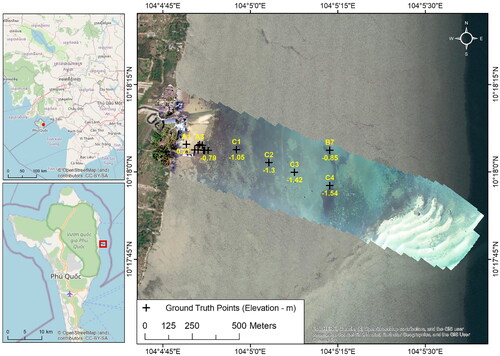
The study site depicted in Figure 1 is in the Bai Bon intertidal flat on the east coast of Phu Quoc Island, in Kien Giang Province, Vietnam. This area is of interest due to the island’s large seagrass beds, which represent more than half of the seagrass in Vietnam. However, previous estimates of the seagrass area have varied widely, from 3,750 hectares to 10,063 hectares, highlighting the uncertainty surrounding the exact area and boundaries of the seagrass, presenting a challenge for blue carbon stock quantification (Nguyen 2008; Vinh et al. 2008; Cao et al. 2012; Nguyen et al. 2014). The seagrass beds are in a turbid coastal region near the mouths of the Mekong River, with a shallow distribution limit of about 3-5 meters. Also, this location is on the overlap between two Sentinel-2 paths, resulting in an average revisit rate of 2.5 days, which provides a unique opportunity for time series analysis. The region of interest covers approximately 66 hectares and more than 1.5 km from the shore towards a sand dune, making it accessible for for UAV flights and field surveys. Five seagrass species were observed in the area, including Halophila ovalis (Ho), Halodule uninervis (Hu), Cymodocea serrulata (Cs), Thalassia hemprichii (Th), Enhalus acoroides (Ea), which are typically found in mixed beds (Figure S1). Seagrasses in the study area have a maximum distribution during the dry season from November to March and may be reduced during the rainy season from April to October (Nguyen 2013).

Figure 1. The study area, with captured UAV image on the background of a true colour image from high resolution satellite, with ground truth points and their elevation in meters.

2.2. Field survey & ground truth

As the intertidal flat was rather shallow (less than 1.6 m deep), the field observations were carried out by walking along the tidal flats to gather information about the benthic type, seagrass species and their density. The team took 16 observations of position (latitude, longitude), time of observation, seagrass species, water depth, density (percentage cover), shoot length, using a GPS logger, several 50 cm quadrats, a 2-m folded ruler, a waterproof camera, and waterproof notes (Table S1). The GPS logger used in this case was an iPhone X with the application called myTracks. The application allowed for recording the GPS location of the phone, and the photo and note of the observation. In recording settings, the Accuracy threshold was set to "Precise", which remove low precision GPS. However, as inaccuracy of the geolocation of 10 m was expected, the field observation and photo were manually compared with the UAV Orthomosaic by visual interpretation (Merry and Bettinger 2019). Percentage cover was estimated by using a 50 × 50 cm quadrats, which were divided into twenty-five 10x10cm grids, if one grid has seagrass present, it is counted for 4%. The field observations the basis for creating training data for the UAV orthomosaic classification described below.

Table 1. List of images used for the analysis.

Index	Date of acquisition	Sensing orbit number	Sensing orbit direction	Spacecraft name	Cloud free area	Estimated tide level (m above mean sea level)
1	2019-11-12	118	DESCENDING	Sentinel-2B	100%	0.164
2	2019-11-15	18	DESCENDING	Sentinel-2B	100%	0.208
3	2019-11-17	118	DESCENDING	Sentinel-2A	87%	0.294
4	2019-11-22	118	DESCENDING	Sentinel-2B	100%	0.211
5	2019-11-27	118	DESCENDING	Sentinel-2A	100%	0.187
6	2019-11-30	18	DESCENDING	Sentinel-2A	100%	0.306
7	2019-12-02	118	DESCENDING	Sentinel-2B	100%	0.289
8	2019-12-07	118	DESCENDING	Sentinel-2A	100%	0.174
9	2019-12-10	18	DESCENDING	Sentinel-2A	100%	0.153
10	2019-12-15	18	DESCENDING	Sentinel-2B	100%	0.258
11	2019-12-20	18	DESCENDING	Sentinel-2A	97%	0.175
12	2019-12-22	118	DESCENDING	Sentinel-2B	100%	0.088
13	2019-12-25	18	DESCENDING	Sentinel-2B	98%	0.139
14	2020-01-01	118	DESCENDING	Sentinel-2B	100%	0.179
15	2020-01-04	18	DESCENDING	Sentinel-2B	100%	0.103
16	2020-01-06	118	DESCENDING	Sentinel-2A	100%	0.085
17	2020-01-09	18	DESCENDING	Sentinel-2A	100%	0.107
18	2020-01-19	18	DESCENDING	Sentinel-2A	100%	0.009
19	2020-01-21	118	DESCENDING	Sentinel-2B	100%	0.011
20	2020-01-24	18	DESCENDING	Sentinel-2B	100%	0.143
21	2020-01-26	118	DESCENDING	Sentinel-2A	99%	0.187
22	2020-02-05	118	DESCENDING	Sentinel-2A	100%	−0.015
23	2020-02-13	18	DESCENDING	Sentinel-2B	100%	0.072
24	2020-02-15	118	DESCENDING	Sentinel-2A	100%	−0.045
25	2020-02-18	18	DESCENDING	Sentinel-2A	85%	−0.099
26	2020-02-20	118	DESCENDING	Sentinel-2B	100%	−0.018
27	2020-02-23	18	DESCENDING	Sentinel-2B	100%	0.095
28	2020-02-25	118	DESCENDING	Sentinel-2A	100%	0.081
29	2020-03-11	118	DESCENDING	Sentinel-2B	100%	0.055
30	2020-03-14	18	DESCENDING	Sentinel-2B	100%	−0.124
31	2020-03-19	18	DESCENDING	Sentinel-2A	100%	−0.136
32	2020-03-21	118	DESCENDING	Sentinel-2B	100%	−0.036
33	2020-03-31	118	DESCENDING	Sentinel-2B	100%	−0.255

2.3. UAV image acquisition and classification

Due to the constantly changing appearance of seagrass in the intertidal flat due to turbidity and tidal dynamics, UAV images were acquired to provide ground truth at the optimal condition, low tide, and clear water, for satellite image analysis. A DJI Phantom 4 Pro UAV with an RGB camera was used for its robustness in a windy coastal environment and high image quality. To capture images at low tide during the daytime, the TOPEX/POSEIDON global tide model was used to estimate the tide level. Referring to the estimation, a field trip was planned during February 4-8, 2020, to match with the low tide. The UAV was flown with a pre-programmed path using DJI GS Pro. Seven flight missions were flown to cover the intertidal flat on 2020-02-05, with the one flown between 15:57 and 16:28 chosen for having the best image quality. During the 29-minute-long flight mission, the tide level was −0.342 m at the beginning and −0.326 m at the end, but the 16 cm difference should not have significantly influenced the orthomosaic. The weather was sunny and some shadows were cast by tall objects, but sun glint was minimal. The images were captured at slightly off-nadir angle to further eliminate sun glint. The altitude was 150 m, resulting in a ground sampling distance of 4.09 cm, which was enabled to resolve individual blades of seagrass. The spatial coverage was 66 hectares, which was equal to the area covered by 6600 pixels of Sentinel-2’s 10 m resolution images. The overlap rate was 86% and the sidelap was 80%. The area included many permanent structures, 4 of which were used as Ground Control Points (GCPs) for georeferencing (Table S5). All 469 captured images were orthormosaicked using Pix4D with default settings. The orthomosaic was then georeferenced in QGIS 3.14 to match the GCPs’ geolocation in the UAV image with the same points in a high-resolution image captured on 2020/3/23 by Maxar Techonologies, accessed via Google Earth. The orthomosaic was subsequently clipped to remove the jagged edges and irrelevant land features and uploaded to Google Earth Engine for further analysis.

Table 5. Correlation between classification accuracy and tide levels.

Pearson correlation between overall accuracy of images without water column correction and tide level	Pearson correlation between overall accuracy of images with water column correction and tide level
−0.351 (p = 0.109)	−0.378 (p = 0.083)

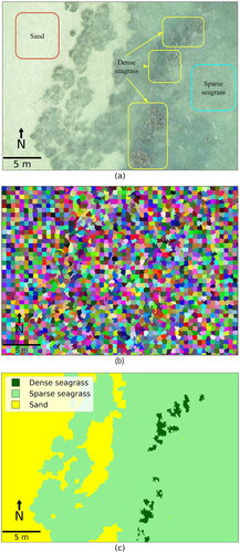
For classification of the orthomosaic, Object-based image analysis (OBIA) was used as it has been found to be superior to pixel-based analysis for seagrass mapping (Roelfsema et al. 2014; Baumstark et al. 2016; Wicaksono and Lazuardi 2018). OBIA is particularly useful in this case, as sun glint or leaf shadows may interfere with seagrass detection by pixel-based classification (Figure 2a). The image segmentation method was Simple Non-Iterative Clustering (SNIC) (Achanta and Susstrunk 2017), implemented in Google Earth Engine, with following parameters: Compactness: 1, Seed size: 15, Connectivity: 8, Neighbourhood size: 8. Those parameters were selected after trials and errors, for producing image objects that resemble the bushes of Enhalus acoroides seagrass (Figure 2b). For each object, the texture information was calculated with the following variables: mean, standard deviation and contrast of the reflectance, perimeter, width, and height of the object.

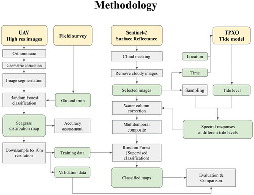
Figure 2. The overall flow chart of image analysis.

Three classes were chosen based reflect the spectral responses of the bottom type: sand, sparse seagrass, and dense seagrass (Figure S3 The difference between sparse and dense seagrass is not simply due to a difference in species, because species such as Cs, Th, Ea appeared to have similar reflectance (Figure 2a, Figures S1 and S2), which is also found by other researchers (Fyfe 2003; Wicaksono et al. 2019). However, their size and density may contribute to the distinction in their reflectance (Figure S3). Sparse seagrass class is seagrass areas with brighter reflectance, which is either comprised of small seagrass species such as Ho, Hu, Cs, Th, or a large seagrass species (Ea) at canopy height lower than 50 cm, or a mix of them (Figure 2a, Figure S1a–g, Table S1). Dense seagrass class is seagrass with darker reflectance, seemingly due to self-shadowing effects and the lack of sand that can be observed, mostly comprised of Ea at high density (100%) and canopy height more than 50 cm (Figure S1h, Table S1). Besides the three classes, features such as boats and houses were excluded from the training data, because they only occur occasionally (17 houses, 1-50 square meter each and 34 boats, 1-10 square meter each) and would eventually not be visible in the Sentinel-2 satellite images.

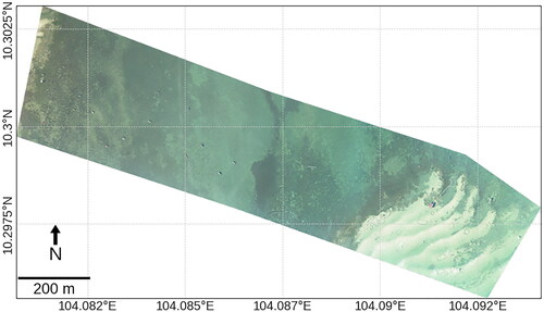
Figure 3. The orthomosaic of the UAV images.

A Random Forest classifier with 100 trees was employed for classification, taking both the spectral and texture information of each pixel as inputs. The choice of 100 trees was deemed optimal showed a good balance between accuracy and computation speed. The training data were created through visual interpretation of the orthomosaic, with reference to the field survey, and consisted of 79 points for sand, 178 points for sparse seagrass, and 186 points for dense seagrass. The training dataset was randomly divided into 70% for training and 30% for validation, with the training portion being utilised to train the classifier. The classifier was used to classify the image, and the classification results were compared with the validation portion to generate a confusion matrix. From the confusion matrix, the overall accuracy, producer’s accuracy, and consumer’s accuracy of each class was calculated.

The UAV image was used as the ground truth for the series of Sentinel-2 images with the assumption that seagrass beds have not changed significantly in the dry season from 2019-11 to 2020-4. Applications of using UAV for validation of satellite remote sensing have been recently explored (Gray et al. 2018; Carpenter et al. 2022). To provide training data and validation for Sentinel-2 image analysis, the classified UAV image was downsampled to a resolution of 10 m. Downsampling was done using the "reduceResolution" method in Google Earth Engine, with the "mode" reducer utilised to produce the most representative class value. The "reduceResolution" method was used to reproject the classified image from its original resolution of 4 cm to the target resolution of 10 m, aligning its projection with the target Sentinel-2 image. The reprojection relied on the mode of all pixels to generate the final output, with the class value of the output pixel being the class with the most pixels in the higher resolution result.

2.4. Tide model TPXO

The tide level was employed to develop parameters for water column correction and to account for the effects of tides on image classification. The TOPEX/POSEIDON global tide model (TPXO) was utilised to estimate the mean sea level datum at the time of satellite image acquisition, as the tide level data from ground stations were inaccessible. The TPXO was developed to assimilate TOPEX/Poseidon altimeter data into a global barotropic tidal model (Dushaw et al. 1997). The Application Programming Interface (API) from worldtides.info was used to run the tide model, which required the location and time as inputs. The location was the centre of the study area (10° 17′ 55.3704” N, 104° 5′ 29.6124” E), and mean sea levels at the nearest grid (10° 19′ 59.88” N, 104° 10′ 1.2” E) were obtained. It was assumed that the tide level was uniform across the 400 m x 1600 m study site and was represented by the value at its centre, which was within one pixel of the TPXO model (1/30-degree resolution). The time input for the model was the date information retrieved from the selected Sentinel-2 images (Table 1), which were acquired at 10:20 am local time.

2.5. Sentinel-2 images analysis

The Sentinel-2 Level 2-A surface reflectance product, which has been calibrated geometrically and radiometrically, was utilised for the analysis. Images from the dry season between 2019-11-01 and 2020-03-31 were selected to observe the maximal seagrass growth and to maintain consistency with the UAV images. It is because during rainy seasons, turbidity tends to increase as a result of high precipitation, which obstructs light from reaching the bottom, leading to low productivity of benthic seagrass and hindering the detection of seagrass with satellite images (Koedsin et al. 2016; Hossain et al. 2019; Hossain and Hashim 2019; Pham et al. 2019). The satellite images were visually inspected to ensure the seagrass distribution was stable during the study period (Figure S4).

Figure 4. (a) Close ups on the UAV image, (b) object-based segmentation result, and (c) classification result.

The Sentinel-2 images were clipped to the same extent as the UAV orthomosaic. Images with more than 15% of the pixels within the area of interest masked as clouds, using the per-pixel cloud probability values embedded in Sentinel-2 level 2 product, were excluded from the analysis. As a result, out of 60 images in the study period, 33 were selected. Table 1 presents the list of images used for classification, along with the tide level is obtained from the tide model as previously described.

The individual images were first pre-processed and then a multitemporal composite was created from a time series of images. For individual images, spectral indices were calculated with emphasis on the spectral response of coastal ecosystem and water column correction. For the multitemporal composite, the percentile value and interval means were calculated from a time series of images. The indices used in this paper are listed in Table 2, with more detailed explanation about them below.

Table 2. List of indices used in this paper.

Index	Equation	Usage
Normalized Difference Vegetation Index (Tucker 1979)	$\mathit{NDVI}= \frac{\mathit{NIR}-\mathit{Red}}{\mathit{NIR}+\mathit{Red}}$	Identifying emerged vegetation
Normalized Difference Water Index (McFeeters 1996)	$\mathit{NDWI}= \frac{\mathit{Green}-\mathit{NIR}}{\mathit{Green}+\mathit{NIR}}$	Identifying water bodies
Modified Normalized Difference Water Index (Xu 2006)	$\mathit{mNDWI}= \frac{\mathit{Green}-\mathit{SWIR}1}{\mathit{Green}+\mathit{SWIR}2}$	Identifying water bodies
Depth Invariant Index (Lyzenga 1981)	${\mathit{DII}}_{ij}=\ln \hspace{0.17em}\left(L_i-L_{si}\right) - \left[\left(\frac{k_i}{k_j}\right) \times \ln \hspace{0.17em}\left(L_j-L_{sj}\right)\right]$	Adjustment for bottom reflectance, explained in detail below.
Percentile (p[i])	The value of the ith percentile in the list	Describing the variation of values within the list
Interval mean (intMn[ij])	The mean of values between the ith percentile and j percentile.	Describing the variation of values within the list

The Normalized Difference Vegetation Index (NDVI), Normalized Difference Water Index (NDWI), Modified Normalized Difference Water Index (mNDWI) were calculated to provide additional information for classification of seagrass in the images. NDVI emphasises the presence of vegetation, while NDWI and mNDWI emphasise the presence of water bodies. Those indices are not typically used for identifying seagrass, due to the strong absorption of the infrared bands by water. However, intertidal sand and seagrass may emerge above the water surface at low tide and display characteristics similar to their terrestrial counterparts, hence those indices were considered in this research.

The Depth Invariant Index (DII) (Lyzenga 1981) was calculated for adjusting the water column effects on the bottom reflectance. Among many water column correction methods, this approach is simple, and requires few input data, while it may increase classification accuracy. Its equation is as follows: $${\mathrm{D}II}_{ij}=\ln \hspace{0.17em}\left(L_i-L_{si}\right)-\left[\left(\frac{k_i}{k_j}\right)\times \ln (L_j-L_{sj})\right]$$

• DII is the Depth Invariant Index, i, j is the name of the respective bands in the pair considered: blue, green or red. BG, BR, GR stands for Blue-Green, Blue-Red and Green-Red respectively.

• L_i is the reflectance of band i at the pixel.

• L_si is the average reflectance of band i over a deep water, this deep-water region is manually sampled further seawards, near the study site.

• k_i is the attenuation coefficient, calculated from the regression of reflectance against depth, results shown in Table 3 below.

Table 3. Theil Sen slope and coefficient of determination (in brackets) between the natural log of blue, green, red, nir, and swir1 against tide levels for Dense seagrass, Sparse seagrass, and Sand.

	Dense seagrass	Sparse seagrass	Sand
lnblue	−0.954 (0.152)	−1.063 (0.193)	-1.674 (0.476)
lngreen	−0.857 (0.121)	−0.866 (0.151)	-1.625 (0.504)
lnred	−0.998 (0.085)	−0.966 (0.091)	-1.785 (0.422)
lnnir	−1.152 (0.099)	−1.150 (0.105)	−1.830 (0.354)
lnswir1	−1.787 (0.146)	−1.825 (0.152)	−1.948 (0.208)
lnswir2	−1.727 (0.145)	−1.712 (0.146)	−2.011 (0.212)

The attenuation coefficients are usually calculated by analysing the attenuation in the reflectance of pairs of bands at different depths over a homogeneous substrate. However, in this study site, the sand pixels appear to be distributed at similar depths, limiting the ability to carry out such regression. As a substitution, the spectral response at different tide levels was used to simulate the changes in depth. As light attenuates in water, the reflectance decreases exponentially against the water depth (Lyzenga 1981). The points from the training data for sand were sampled for each image, and their mean was used to represent the sand’s reflection. The natural logarithms of spectral responses of the blue, green, and red bands in the sandy pixels were regressed against the tide level at the time of image acquisition (Figure 3, Table 3). The substrate type, solar radiation, sea surface temperature, pH, and salinity were assumed to remain relatively stable throughout the study period. As noise is expected, the Theil-Sen robust linear regression was used (Theil 1950; Sen and Kumar Sen 1968). The resulting attenuation coefficients were used for the calculation of the DII. The newly calculated DII for each band pair - Blue-Green (DII_BG), Blue-Red (DII_BR) and Green-Red (DII_GR) - were added to the image for further analysis.

To thoroughly comprehend the variation of the intertidal flat due to tidal dynamics, a method from (Murray et al. 2019) was adapted, creating a multitemporal composite from a series of images. The frequent image acquisition of the Sentinel-2 constellation at this location, with one image captured every 2.5 days, enabled a comprehensive analysis of the tidal stage variation. The variation of spectral responses in each class was unique (Figure S5). A multitemporal composite was created by calculating 12 variables to represent the variation of each pixel across the 33 images for each of the pixel in the image, including: six reflectance bands: blue, green, red, nir, swir1, swir2; three multi-spectral indices: NDVI, NDWI, mNDWI; three DII: DII_BG, DII_BR, DII_GR. For each of those band, 17 covariates were calculated to describe the variation: min, max, stdDev, mean, 10th, 25th, 50th, 75th and 90th percentile (p10, p25, p50, p75, p90); the interval means (intMn0010, intMn1025, intMn2550, intMn5075, intMn7590, intMn90100, intMn1090, intMn2575). Equations for calculating each covariate are listed in Table 2.

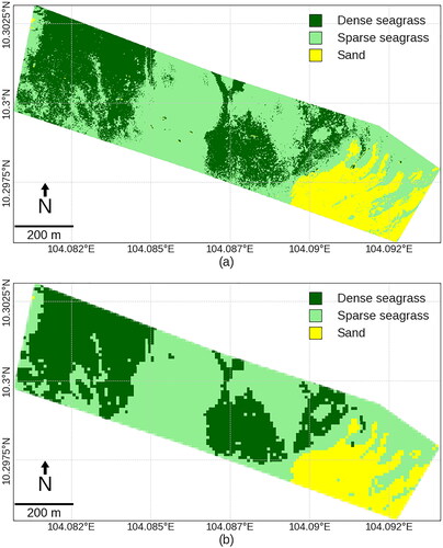
Figure 5. (a) The classification of the orthomosaic, and (b) the downsampled classification result of the UAV images.

The Sentinel-2 images were then classified using the training data obtained from the UAV images. Stratified sampling was performed on the UAV orthomosaic to obtain 100 points from each class, which were then used as the training data for the Sentinel-2 images classification. Classification was done using the Random Forest classifier with 100 trees as the parameter, similar to the UAV classification. Four classification schemes were executed to evaluate the effects of water column correction and the usage of multitemporal composites on classification accuracy, with the inputs for classification described in Table 4. For single-image analysis, each image listed in Table 1 was classified, with and without water column correction. For the multitemporal composites from the 33 images, the 17 covariates listed above were used as inputs instead of the reflectance values and indices themselves to emphasise the variation within the stack of images rather than just their mean values.

Table 4. Table of inputs for classification.

Image	Inputs for classification
Single images without water column correction	Six reflectance bands (blue, green, red, near infrared band, and shortwave infrared 1 and shortwave infrared 2)
Single images with water column correction	The above six reflectance bands and three Depth Invariant Indices: DII_BG, DII_BR, DII_GR
The multitemporal composite without water column correction	The 17 covariates for the above six reflectance bands and three multi-spectral indices (NDVI, NDWI, mNDWI)
The multitemporal composite with water column correction	The 17 covariates for each of the above six reflectance bands, three multi-spectral indices (NDVI, NDWI, mNDWI), and three Depth Invariant Indices.

For classification accuracy assessment, the training data was randomly split to 70% for training and 30% for validation. The split was repeated 100 times to produce confusion matrices and calculate the average accuracy. The overall accuracy went through a Pearson correlation test against the tide levels to reveal any correlations between the two variables. The comparisons between the overall accuracy of classified maps based on single images with and without water column correction, as well as the overall accuracy of classified maps based on multitemporal composites with and without water column correction was presented. The methodology is summarised in Figure 4.

3. Results

3.1. UAV image acquisition and processing

As depicted in Figures 2 and 5, the high-resolution UAV image can reveal features of the seagrass canopy. Enhalus acoroides can grow tall enough to emerge above the water surface at low tide, revealing the contrast of seagrass leaves and their shadows. The size of the object segmented by the SNIC algorithm is approximately 60 cm, which is similar to the size of an Ea canopy. In areas with homogeneous reflectance, such as the sandy area, objects resemble squares. In areas with heterogenous reflectance, such as at the edge between sand and seagrass, or between two kinds of seagrasses, objects may have elongated shapes which conform with the seagrass canopy. The contrast of the leaves and their shadows is an important object feature that influences the classification process.

Figure 6 illustrates the classification result, showing the irregular pattern of distribution of dense and sparse seagrass, with dense seagrass appearing to cluster into continuous patches. The accuracy assessment (Table S2) yielded a mean overall accuracy of 98.11%, indicating a high degree of consistency between the training data and classified results. However, at the transition between the two classes, the dense and sparse seagrass was occasionally misclassified as each other, possibly due to their similar appearance. Additionally, visual inspection suggests that random errors occurred, such as boats or houses being classified as sand, and their shadows being classified as seagrass. To match the resolution of Sentinel-2 images, the classified results were downsampled to 10 m using the mode as the reducer. The downsampling process seemed to have largely removed random errors in classification.

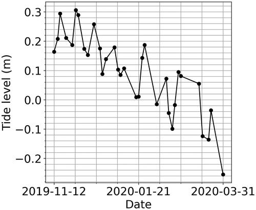
Figure 6. Tide levels at image acquisition time (10:20 am local time) for the Sentinel-2 images analysed.

3.2. Sentinel-2 images analysis

The Sentinel-2 images captured a range of tidal variation from 0.306 m (on 2019-11-30) to −0.255 m (on 2020-03-31) above mean sea level. (Figure 7). This variation in tide levels may cause intertidal features to be exposed during low tide, affecting their appearance and consequently, the classification process.

Figure 7. True colour composite and classified images from Sentinel-2 satellites at high and low tides. (a), (b), and (c) show the true colour composite. (d), (e), (f) show the classification result without water column correction and (g), (h), (i) show the classification result with water column correction. (a), (d), (g) are captured at low tide, (b), (e), (h) at medium tide and (c), (f), (i) at high tide.

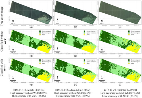
Figure 8 shows the images and classification results at different tide levels. At lower tides (a), the reflectance from the bottom can be seen more clearly than at higher tide (c). Sandy bottom, shown in bright to the east shows the clearest difference in reflectance as tide level changes. Sparse seagrass (light green) and dense seagrass (dark green) are better distinguished at medium or low tide (d, e, g, h). At high tide, especially when the water is optically deep, the distinction between sparse and dense seagrass is challenging (f, i).

Figure 8. Logarithms of reflectance of the blue, green, red, near infrared, short-wave infrared 1 and short-wave infrared 2 of Dense seagrass, Sparse seagrass, and Sand at different tide levels. Red lines show the regression slope of a Theil Sen Robust regression.

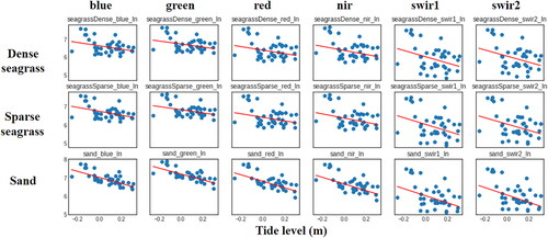
The regression analysis reveals negative correlation between the logarithms of reflectance values and tide levels (Figure 3) for all bands and all bottom types, indicating that the reflectance values at decrease with increasing tide levels. However, points at low tide levels seem to deviate from the trends, with higher reflectance values than predicted, possibly due to the exposure of the intertidal flat during low tide. The correlation has different degrees of strength, shown by the coefficient of determination values from 0.085 to 0.504 (Table 3). Sand seems to have a stronger correlation, especially in the optical bands (red, green, blue), as the coefficients of determination are closer to 1. Those three correlation coefficients were used as attenuation for water column correction to calculate the DII values.

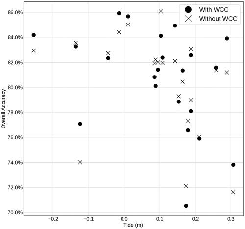
Figure 9 shows that at higher tide levels, lower classification accuracy was achieved, while most of the images captured at lower tide yielded an overall classification accuracy above 82%. Examples of confusion matrices for an image could be found in Tables S3 and S4. Table 5 shows a weak negative relation between tide levels and classification accuracy, both with and without water column correction. The reason for this could be that at lower tide levels, the bottom reflectance is higher as it is less absorbed by the water column, leading to better separation of the classes. At higher tide levels, the water column absorbs more of the upwelling reflectance, impeding the performance of the classifier, which in turn leads to lower accuracy. An example of low accuracy at high tide could be observed in Figure 8c.

Figure 9. Overall accuracy of classification results of seagrass at different tide levels for images with and without water column correction.

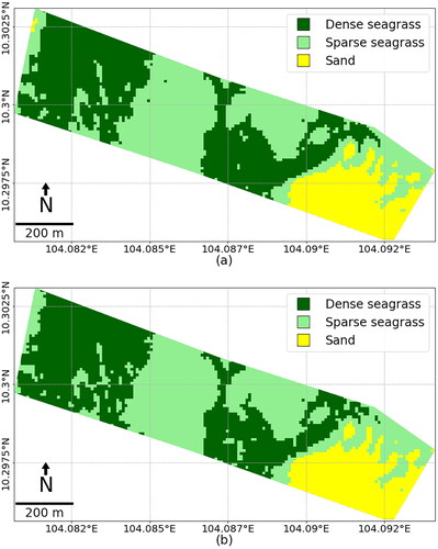
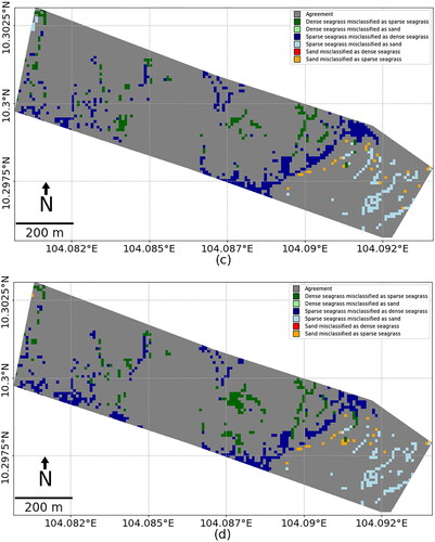
Figure 10 demonstrates the classification results from the multitemporal composite and the difference map from results derived from UAV images. These results are in good agreement with the classification results from UAV (Figure 6), indicating high accuracy. Figure 10(c) and (d) highlight misclassifications in transition zone between dense and sparse seagrass, and between sparse seagrass and sand, but rarely between dense seagrass and sand. The classification using multitemporal composites can achieve high accuracy, and there is no significant difference in the results with or without water column correction.

Figure 10. Classification results from the multitemporal composite, (a) without WCC and (b) with WCC and the difference map from UAV classified image with the multitemporal composite (c) without WCC and (d) with WCC.

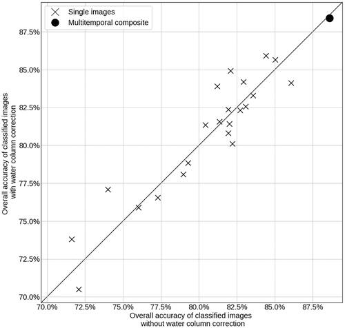
Water column correction had minimal improvement in accuracy for mapping seagrass on an intertidal flat in this study (Figure 11). The average accuracy for classification of images without water column is 80.4%, while with water column correction, it is higher slightly higher at 80.6%. Visual interpretation (Figure S6) suggests that the water column is optically deep in some images, which may obscure the bottom type and lead to low accuracy with or without water column correction. There were cases where the accuracy of the image with water column correction was higher than without (Figure S7). The opposite is also true, as there are cases where the accuracy of the images with WCC have lower accuracy than those without. However, using the multitemporal composite does improve accuracy, with an overall accuracy of 88.4% for the composite without water column correction, and 88.6% with water column correction, signifying an 8% improvement in both cases. This accuracy is higher than the highest accuracy of classification for single images without water column correction (86.1%) and with water column correction (85.9%).

Figure 11. Comparison between the classification accuracy of images with and without water column corrections, and between classifying single images and the multitemporal composite.

4. Discussion

4.1. Relationship between tide levels and classification accuracy

Classifying images at lower tide level appears to result in higher classification accuracy, as shown in Figure 9 and Table 5. This is perhaps due to the shallower water column during low tide, allowing more bottom reflectance to reach the satellite sensors. This results in better distinction between seagrass and sandy pixels, which in turns leads to better accuracy. Therefore, it highlights the necessity to consider tidal stages while selecting images for classification.

While some may argue that choosing the right image, with optimal conditions such as low tide and low turbidity, is sufficient in improving the classification accuracy, this approach has limitations. Firstly, the criteria for selecting such images are not universal and depend on various factors. Previous studies (Hossain et al. 2019) have attempted to filter for such images based on criteria such as tide level thresholds and low turbidity level represented by a low Normalized Difference Turbidity Index (NDTI) (Lacaux et al. 2007). However, NDTI can be affected by bottom reflectance and may not directly correlate with turbidity. Secondly, even if an image is selected based on those threshods, parts of the image could have contamination, such as cloud or local turbidity. Therefore, an approach can account for tidal dynamics in classification for the whole image is desirable.

4.2. Development of a classification method using multitemporal composite

Our results suggest that using a machine learning classifier on the multitemporal composite could provide the more benefits than water column correction, while simplifying data processing. However, the robustness of the method needs to be further discussed, particularly in terms of how the quantity and quality of available images may impact the classification accuracy. In the present study, 33 images were used over a 5-month period, which may not be feasible for datasets with lower revisit periods such as Landsat. In such cases, image selection criteria may need to be adjusted to include more images for meaningful multi-temporal compositing, such as extending the study period across multiple years, although there is a limit to how much compromising can be done given the rapidly changing nature of seagrass ecosystems. Nevertheless, with the increasing availability of satellite images, recent and future changes to seagrass beds can be quantified with higher accuracy.

UAV images played a crucial role in this framework, as the high spatial resolution and the flexible timing of image acquisition provides accurate training data, serving as a cost-effective supplement to ground truth data collected through field surveying (Gray et al. 2018; Komatsu et al. 2020; Carpenter et al. 2022). It was important to capture the image at low tide because the tall seagrass canopy could be clearly observed, validating their appearance in the satellite image. However, there are several limitations to using UAVs for mapping seagrass. The spatial coverage of UAV images is currently limited compared to satellite imagery, due to scalability constraints such as the short time window for capturing images, limitation in resources. Furthermore, there are limitations for assembling UAV images over the water surface. Ortho-mosaicking requires images to have matching features, which is a difficult condition to achieve, as the water surface constantly and chaotically moves. In the UAV images presented in this paper, seagrasses in the deeper areas were not captured. Therefore, for broader application of this method, substitutes for UAV images could be reconsidered, such as high-resolution satellite image, unmanned underwater vehicles, or side scan sonars.

4.3. Comparison among methods for improving classification accuracy

In this study, water column correction did not significantly improve classification accuracy, in both the classification using single images and the multitemporal composite. Water column correction is known to have limited effectiveness in shallow and turbid waters (Uhrin and Townsend 2016). In our approach, the weak correlation between tidal level and reflectance was possibly due to the small tidal variation of 0.6 m or a non-linear relationship. In addition, water quality fluctuations among images could have further hindered the effectiveness of water column correction.

In contrast, the multitemporal composite approach resulted in a larger improvement in accuracy, with an 8% compared to the average and 2% higher than the highest accuracy obtained from single image classification. This suggests that using multitemporal composite is superior to water column correction for improving classification accuracy on intertidal flats. This improvement to 88% accuracy is significant for seagrass mapping, as most studies have been reporting up to 80% accuracy to be high for multispectral seagrass mapping (Hossain et al. 2015; Pham et al. 2019). However, caution must be exercised with overfitting due to the large number of inputs (12 bands multiplied by 17 covariates) for training the classifier, which may undermine the method’s robustness when applying to other areas.

4.4. Broader implications and future work

As the protocol seems to perform well in this location, it is potential to do a time series analysis over decades of currently available imagery to explore change over time, establishing inventories for seagrass distribution. Also, the usage of the multitemporal composite was successful in mapping intertidal flats globally (Murray et al. 2019), and its effectiveness in seagrass mapping beds on tidal flats were discussed in this research. There are potentials for this approach to be applied in a larger region for automatic identification of seagrass beds worldwide.

The current method showed a significant improvement in classification accuracy for an intertidal flat with turbid water. This is an important habitat to quantify well in Vietnam because the majority of seagrass in Vietnam are in this type of habitat (Nguyen 2008; 2013). Furthermore, many countries in the Indo Pacific Ocean region have a similar condition, where potentially highly productive ecosystems are yet to be quantified. (Unsworth et al. 2019) As UAV imagery, Tidal data, and Satellite datasets having high quality and are becoming more accessible, the protocol could help to quantify the remaining uncertainties in tropical seagrass ecosystems. Such development will help advance the understanding of marine carbon cycles and contribute to tackling climate change. However, there are various habitats for seagrass, such as in bays, lagoons, or other coastal areas. This method’s applicability to those habitats needs further research.

This research opened the possibility to consider more applications of using the multitemporal composites for seagrass mapping. Besides improving classification accuracy, by analysing the change over time of the reflectance of seagrass beds, it is possible to quantify its exposure to photosynthesis active radiation, helping to understand more about its primary production and carbon sequestration efficiency. The changes of reflectance in relation to tide levels could be used for shallow bathymetry. The abruptly high reflectance in NIR or SWIR at lower tide levels could perhaps signify emergence of the intertidal flat above the water surface. In this study site, parts of the intertidal flats, especially the sandy area, the short seagrass adjacent to the sandy shore seagrass, and the tall seagrass canopy occasionally emerged from the water surface at low tide. Even though still uncertain, such emergence has some possibilities to be observed by satellite images. That signifies the potential to use a time series with various tide levels to analyse the shallow bathymetry. This is significant as shallow bathymetry is challenging to measure by field surveys, and current bathymetry estimation from satellite images have been majorly done on analysing a single image (Dierssen et al. 2003; Lyzenga et al. 2006; Traganos et al. 2018).

In addition, while downscaling the UAV orthomosaic, it was possible to provide the percentage cover of seagrass (Price et al. 2022). Though this paper did not focus on quantifying seagrass primary production, this could be used for further analysis, as density, species, and canopy heights are important parameters to quantify biomass and photosynthesis (Stankovic et al. 2018).

5. Conclusion

This paper aimed to improve seagrass mapping on an intertidal flat, using a combination of UAV images, tidal data, and satellite images. High-resolution UAV images were analysed using Obect Based Image Analysis and Random Forest classifier to produce accurate training data. Tidal data from the TPXO model were used for water column correction, slightly improving the classification accuracy of satellite images by 0.2% on average. In contrast, the multitemporal composite approach, developed using statistical covariates of the time series of Sentinel-2 image resulted in an overall accuracy of 88.4%, 8% higher overall accuracy compared to single image classification, regardless of water column correction. The study confirmed the hypothesis that using multitemporal composites improved classification accuracy for seagrass mapping on intertidal flats. This protocol could be applied to advance seagrass distribution mapping, especially in challenging areas waters.

Data availability statement

Sentinel-2 datasets were obtained from Google Earth Engine data catalogue at https://developers.google.com/earth-engine/datasets/catalog/sentinel

TPXO Tide model data were obtained from the API at https://www.worldtides.info/

The UAV images, JavaScript and Python code for processing are available on request from the author.

Disclosure statement

No potential conflict of interest was reported by the authors.

References

- Achanta R, Susstrunk S. 2017. Superpixels and polygons using simple non-iterative clustering. In Proceedings of the IEEE conference on computer vision and pattern recognition. 4651–4660.
- Baumstark R, Duffey R, Pu R. 2016. Mapping seagrass and colonized hard bottom in Springs Coast, Florida using WorldView-2 satellite imagery. Estuar Coast Shelf Sci. 181:83–92.
- Borfecchia F, Micheli C, Carli F, de Martis SC, Gnisci V, Piermattei V, Belmonte A, de Cecco L, Martini S, Marcelli M. 2013. Mapping spatial patterns of posidonia oceanica meadows by means of daedalus ATM airborne sensor in the coastal area of Civitavecchia (Central Tyrrhenian Sea, Italy). Remote Sens. 5(10):4877–4899. [accessed 2022 November 21].
- Cao VL, Nguyen VT, Komatsu T, Nguyen DV, Dam DT. 2012. Status and threats on seagrass beds using GIS in Vietnam. Remote Sens Marine Environ II. 8525(October):852512.
- Carpenter S, Byfield V, Felgate SL, Price DM, Andrade V, Cobb E, Strong J, Lichtschlag A, Brittain H, Barry C, et al. 2022. Using unoccupied aerial vehicles (UAVs) to map seagrass cover from sentinel-2 imagery. Remote Sens. 14(3):477. [accessed 2022 November 21].
- Costanza R, Arge R, DeGroot R, Farberk S, Grasso M, Hannon B, Limburg K, Naeem S, Neill RVO, Paruelo J, et al. 1997. The value of the world ’ s ecosystem services and natural capital. Nature. 387(May):253–260.
- Costanza R, de Groot R, Sutton P, van der Ploeg S, Anderson SJ, Kubiszewski I, Farber S, Turner RK. 2014. Changes in the global value of ecosystem services. Global Environ Change. 26(1):152–158.
- Cullen-Unsworth L, Unsworth R. 2013. Seagrass meadows, ecosystem services, and sustainability. Environment. 55(3):14–28.
- de Groot R, Brander L, van der Ploeg S, Costanza R, Bernard F, Braat L, Christie M, Crossman N, Ghermandi A, Hein L, et al. 2012. Global estimates of the value of ecosystems and their services in monetary units. Ecosyst Serv. 1(1):50–61.
- Dewsbury BM, Bhat M, Fourqurean JW. 2016. A review of seagrass economic valuations: gaps and progress in valuation approaches. Ecosyst Serv. 18:68–77.
- Dierssen HM, Bostrom KJ, Chlus A, Hammerstrom K, Thompson DR, Lee Z. 2019. Pushing the limits of seagrass remote sensing in the turbid waters of Elkhorn Slough, California. Remote Sens (Basel). 11(14):13–15.
- Dierssen HM, Zimmerman RC, Leathers RA, Downes TV, Davis CO. 2003. Ocean color remote sensing of seagrass and bathymetry in the Bahamas Banks by high-resolution airborne imagery. Limnol Oceanogr. 48(1 II):444–455.
- Duarte CM. 2002. The future of seagrass meadows. Environ Conserv. 29(2):192–206.
- Duarte CM, Marbà N, Gacia E, Fourqurean JW, Beggins J, Barrón C, Apostolaki ET. 2010. Seagrass community metabolism: assessing the carbon sink capacity of seagrass meadows. Global Biogeochem Cycles. 24(4):1–8.
- Duffy JE, Benedetti-Cecchi L, Trinanes J, Muller-Karger FE, Ambo-Rappe R, Boström C, Buschmann AH, Byrnes J, Coles RG, Creed J, et al. 2019. Toward a Coordinated Global Observing System for Seagrasses and Marine Macroalgae. Front Mar Sci. 6:317. [accessed 2019 July 10].
- Duffy JP, Pratt L, Anderson K, Land PE, Shutler JD. 2018. Spatial assessment of intertidal seagrass meadows using optical imaging systems and a lightweight drone. Estuar Coast Shelf Sci. 200:169–180.
- Dushaw BD, Egbert GD, Worcester PF, Cornuelle BD, Howe BM, Metzger K. 1997. A TOPEX/POSEIDON global tidal model (TPXO.2) and barotropic tidal currents determined from long-range acoustic transmissions. Prog Oceanogr. 40(1–4):337–367.
- Ellis SL, Taylor ML, Schiele M, Letessier TB. 2021. Influence of altitude on tropical marine habitat classification using imagery from fixed-wing, water-landing UAVs. Remote Sens Ecol Conserv. 7(1):50–63. [accessed 2022 January 28].
- Fourqurean JW, Duarte CM, Kennedy H, Marbà N, Holmer M, Mateo MA, Apostolaki ET, Kendrick GA, Krause-Jensen D, McGlathery KJ, et al. 2012. Seagrass ecosystems as a globally significant carbon stock. Nat Geosci. 5(7):505–509.
- Fyfe SK. 2003. Spatial and temporal variation in spectral reflectance: are seagrass species spectrally distinct? Limnol Oceanogr. 48(1 II):464–479.
- Gillanders BM. 2007. Seagrasses, fish, and fisheries. Seagrasses: Biology, Ecology and Conservation. Dordrecht: Springer.
- Gray PC, Ridge JT, Poulin SK, Seymour AC, Schwantes AM, Swenson JJ, Johnston DW. 2018. Integrating drone imagery into high resolution satellite remote sensing assessments of estuarine environments. Remote Sens. 10(8):1257.
- Green EP, Mumby PJ, Edwards AJ, Clark CD. 2000. Remote sensing handbook for tropical coastal management. United Nations Educational, Scientific and Cultural Organization (UNESCO).
- Hansen MC. 2013. High-resolution global maps of 21st-century forest cover change. Science 342:850–854.
- Hossain MS, Bujang JS, Zakaria MH, Hashim M. 2015. The application of remote sensing to seagrass ecosystems: an overview and future research prospects. Int J Remote Sens. 36(1):61–114.
- Hossain MS, Hashim M. 2019. Potential of Earth Observation (EO) technologies for seagrass ecosystem service assessments. Int J Appl Earth Observ Geoinform. 77:15–29.
- Hossain MS, Hashim M, Bujang JS, Zakaria MH, Muslim AM. 2019. Assessment of the impact of coastal reclamation activities on seagrass meadows in Sungai Pulai estuary, Malaysia, using Landsat data (1994–2017). Int J Remote Sens. 40(9):3571–3605. [accessed 2019 July 10].
- Jia M, Wang Z, Mao D, Ren C, Wang C, Wang Y. 2021. Rapid, robust, and automated mapping of tidal flats in China using time series Sentinel-2 images and Google Earth Engine. Remote Sens Environ. 255:112285.
- Koedsin W, Intararuang W, Ritchie RJ, Huete A. 2016. An integrated field and remote sensing method for mapping seagrass species, cover, and biomass in Southern Thailand. Remote Sens (Basel). 8(4):292.
- Komatsu T, Hashim M, Nurdin N, Noiraksar T, Prathep A, Stankovic M Son T, Thu P, Luong C, Wouthyzen S. 2020. Practical mapping methods of seagrass beds by satellite remote sensing and ground truthing. Coast Mar Sci. 43(1):1–25.
- Lacaux JP, Tourre YM, Vignolles C, Ndione JA, Lafaye M. 2007. Classification of ponds from high-spatial resolution remote sensing: application to Rift Valley Fever epidemics in Senegal. Remote Sens Environ. 106(1):66–74.
- Laengner ML, Siteur K, van der Wal D. 2019. Trends in the seaward extent of saltmarshes across Europe from long-term satellite data. Remote Sens 11(14):1653. [accessed 2022 January 28].
- Lee Z, Carder KL, Mobley CD, Steward RG, Patch JS. 1999. Hyperspectral remote sensing for shallow waters: 2 Deriving bottom depths and water properties by optimization. Appl Opt. 38(18):3831–3843.
- Lefebvre A, Thompson CEL, Collins KJ, Amos CL. 2009. Use of a high-resolution profiling sonar and a towed video camera to map a Zostera marina bed, Solent, UK. Estuar Coast Shelf Sci. 82(2):323–334.
- Li Q, Jin R, Ye Z, Gu J, Dan L, He J, Christakos G, Agusti S, Duarte CM, Wu J. 2022. Mapping seagrass meadows in coastal China using GEE. Geocarto Int. [Internet]. Geocarto Int. 37(26):12602-12617.https://www.tandfonline.com/action/showCitFormats?doi=10.1080%2F10106049.2022.2070672.
- Lyons MB, Roelfsema CM, Kennedy EV, Kovacs EM, Borrego-Acevedo R, Markey K, Roe M, Yuwono DM, Harris DL, Phinn SR, et al. 2020. Mapping the world’s coral reefs using a global multiscale earth observation framework. Remote Sens Ecol Conserv. [Internet]6(4):557–568. [accessed 2022 January 28].
- Lyzenga DR. 1978. Passive remote sensing techniques for mapping water depth and bottom features. Appl Opt. 17(3):379–383.
- Lyzenga DR. 1981. Remote sensing of bottom reflectance and water attenuation parameters in shallow water using aircraft and landsat data. Int J Remote Sens. 2(1):71–82.
- Lyzenga DR, Malinas NP, Tanis FJ. 2006. Multispectral bathymetry using a simple physically based algorithm. IEEE Trans Geosci Remote Sens. 44(8):2251–2259.
- Matsunaga T, Hoyano A, Mizukami Y. 2000. Monitoring of coral reefs on Ishigaki Island in Japan using multitemporal remote sensing data. Hyperspectral Remote Sens Ocean. 4154:212–222.
- McFeeters SK. 1996. The use of the Normalized Difference Water Index (NDWI) in the delineation of open water features. Int J Remote Sens. 17(7):1425–1432.
- McLeod E, Chmura GL, Bouillon S, Salm R, Björk M, Duarte CM, Lovelock CE, Schlesinger WH, Silliman BR. 2011. A blueprint for blue carbon: toward an improved understanding of the role of vegetated coastal habitats in sequestering CO2. Front Ecol Environ. 9(10):552–560.
- Merry K, Bettinger P. 2019. Smartphone GPS accuracy study in an urban environment. PLoS One. 14(7):e0219890.
- Mitra A, Zaman S. 2015. Blue carbon reservoir of the blue planet. (pp. 1-299). New Delhi: Springer.
- Miyajima T, Hori M, Hamaguchi M, Shimabukuro H, Adachi H, Yamano H, Nakaoka M. 2015. Geographic variability in organic carbon stock and accumulation rate in sediments of East and Southeast Asian seagrass meadows. Global Biogeochem Cycles. 29(4):397–415.
- Mumby PJ, Clark CD, Green EP, Edwards AJ. 2010. Benefits of water column correction and contextual editing for mapping coral reefs. Int J Remote Sens 19(1):203–210. https://doi.org/10.1080/014311698216521 [Internet]. [accessed 2022 January 28]
- Murray NJ, Phinn SR, DeWitt M, Ferrari R, Johnston R, Lyons MB, Clinton N, Thau D, Fuller RA. 2019. The global distribution and trajectory of tidal flats. Nature. 565(7738):222–225.
- Nahirnick NK, Reshitnyk L, Campbell M, Hessing-Lewis M, Costa M, Yakimishyn J, Lee L. 2019. Mapping with confidence; delineating seagrass habitats using Unoccupied Aerial Systems (UAS). Remote Sens Ecol Conserv. 5(2):121–135. [Internet]. [accessed 2022 January 28].
- Nellemann C, Corcoran E. 2009. Blue carbon : the role of healthy oceans in binding carbon : a rapid response assessment. UNEP/Earthprint.
- Nguyen VT. 2008. Seagrass in the South China Sea. Hai Phong, Vietnam: Vietnamese Academy of Science and Technology. 1–36. http://www.unepscs.org/components/com_remository_files/downloads/National-Report-Seagrass-Vietnam.pdf [accessed 2023 March 4].
- Nguyen VT. 2013. Nguon loi tham co bien Viet Nam [Seagrass resources of Viet Nam]. Khoa Hoc Tu Nhien va Cong Nghe. 35–67.
- Nguyen DTH, Tripathi NK, Gallardo WG, Tipdecho T. 2014. Coastal and marine ecological changes and fish cage culture development in Phu Quoc, Vietnam (2001 to 2011). Geocarto Int. 29(5):486–506.
- Pendleton L, Donato DC, Murray BC, Crooks S, Jenkins WA, Sifleet S, Craft C, Fourqurean JW, Kauffman JB, Marbà N, et al. 2012. Estimating global “blue carbon” emissions from conversion and degradation of vegetated coastal ecosystems. PLoS One. 7(9):e43542.
- Pham TD, Xia J, Ha NT, Bui DT, Le NN, Tekeuchi W. 2019. A review of remote sensing approaches for monitoring blue carbon ecosystems: mangroves, seagrassesand salt marshes during 2010–2018. Sensors (Basel). 19(8):1933.
- Phinn S, Roelfsema C, Kovacs E, Canto R, Lyons M, Saunders M, Maxwell P. 2018. Mapping, monitoring and modelling seagrass using remote sensing techniques. Seagrasses of Australia: Structure, Ecology and Conservation, 445–487.
- Price DM, Felgate SL, Huvenne VAI, Strong J, Carpenter S, Barry C, Lichtschlag A, Sanders R, Carrias A, Young A, et al. 2022. Quantifying the intra-habitat variation of seagrass beds with unoccupied aerial vehicles (UAVs). Remote Sens. 14(3):480. [accessed 2022 November 21].
- Roelfsema CM, Lyons M, Kovacs EM, Maxwell P, Saunders MI, Samper-Villarreal J, Phinn SR. 2014. Multi-temporal mapping of seagrass cover, species and biomass: a semi-automated object based image analysis approach. Remote Sens Environ. 150:172–187.
- Sagawa T, Boisnier E, Komatsu T, Ben Mustapha K, Hattour A, Kosaka N, Miyazaki S. 2010. Using bottom surface reflectance to map coastal marine areas: a new application method for Lyzenga’s model. Int J Remote Sens. 31(12):3051-3064.
- Sen PK, Kumar Sen P. 1968. Estimates of the regression coefficient based on Kendall’s Tau. J Am Stat Assoc. 63:1379–1389. [accessed 2022 November 21].
- Short FT. 2004. World atlas of seagrasses. Choice Rev. 41(06):41–3160–41-3160.
- Stankovic M, Tantipisanuh N, Rattanachot E, Prathep A. 2018. Model-based approach for estimating biomass and organic carbon in tropical seagrass ecosystems. Mar Ecol Prog Ser. 596:61–70. [accessed 2022 April 26].
- Stumpf RP, Holderied K, Sinclair M. 2003. Determination of water depth with high-resolution satellite imagery over variable bottom types. Limnol Oceanogr. 48(1part2):547–556. [accessed 2022 Januay 28].
- Sudo K, Quiros TEAL, Prathep A, van Luong C, Lin HJ, Bujang JS, Ooi JLS, Fortes MD, Zakaria MH, Yaakub SM, et al. 2021. Distribution, temporal change, and conservation status of tropical seagrass beds in Southeast Asia: 2000–2020. Front Mar Sci. 8(July):637722.
- Tamondong AM, Blanco AC, Fortes MD, Nadaoka K. 2013. Mapping of seagrass and other benthic habitats in Bolinao, Pangasinan using Worldview-2 satellite image. International Geoscience and Remote Sensing Symposium (IGARSS):1579–1582.
- Tamondong AM, Cruz CA, Guihawan J, Garcia M, Quides RR, Cruz JA, Blanco AC. 2018. Remote sensing-based estimation of seagrass percent cover and LAI for above ground carbon sequestration mapping. 1077803.
- Theil H. 1950. A rank-invariant method of linear and polynominal regression analysis (Parts 1-3). Ned Akad Wetensch Proc Ser A. 53:1397–1412. [accessed 2022 November 21].
- Traganos D, Aggarwal B, Poursanidis D, Topouzelis K, Chrysoulakis N, Reinartz P. 2018. Towards global-scale seagrass mapping and monitoring using Sentinel-2 on Google Earth Engine: the case study of the Aegean and Ionian Seas. Remote Sens (Basel). 10(8):1227.
- Traganos D, Poursanidis D, Aggarwal B, Chrysoulakis N, Reinartz P. 2018. Estimating satellite-derived bathymetry (SDB) with the Google Earth Engine and sentinel-2. Remote Sens (Basel). 10(6):1–18.
- Traganos D, Reinartz P. 2018. Mapping Mediterranean seagrasses with Sentinel-2 imagery. Mar Pollut Bull. 134(March):197–209.
- Tucker CJ. 1979. Red and photographic infrared linear combinations for monitoring vegetation. Remote Sens Environ. 8(2):127–150.
- Uhrin A v, Townsend PA. 2016. Improved seagrass mapping using linear spectral unmixing of aerial photographs. Estuar Coast Shelf Sci. 171:11–22. [accessed 2019 July 3].
- Unsworth RKF, Cullen LC. 2010. Recognising the necessity for Indo-Pacific seagrass conservation. Conserv Lett. 3(2):63–73.
- Unsworth RKF, McKenzie LJ, Collier CJ, Cullen-Unsworth LC, Duarte CM, Eklöf JS, Jarvis JC, Jones BL, Nordlund LM. 2019. Global challenges for seagrass conservation. Ambio. 48(8):801–815. [accessed 2019 June 25].
- Unsworth RKFF, Ambo-Rappe R, Jones BL, la Nafie YA, Irawan A, Hernawan UE, Moore AM, Cullen-Unsworth LC. 2018. Indonesia’s globally significant seagrass meadows are under widespread threat. Sci Total Environ. 634:279–286.
- Ventura D, Bonifazi A, Gravina MF, Belluscio A, Ardizzone G, Ventura D, Bonifazi A, Gravina MF, Belluscio A, Ardizzone G. 2018. Mapping and classification of ecologically sensitive marine Habitats Using Unmanned Aerial Vehicle (UAV) Imagery and Object-Based Image Analysis (OBIA). Remote Sens (Basel). 10(9):1331. [accessed 2019 July 2].
- Vinh MK, Shrestha R, Berg H. 2008. GIS-aided marine conservation planning and management: a case study in Phuquoc Island, Vietnam. International Symposium on Geoinformatics for Spatial Infrastructure Development in Earth and Allied Sciences:6.
- Vo TT, Lau K, Liao LM, Nguyen XV. 2020. Satellite image analysis reveals changes in seagrass beds at Van Phong Bay, Vietnam during the last 30 years. Aquat Living Resour. 33(May):4.
- Waycott M, Duarte CM, Carruthers TJB, Orth RJ, Dennison WC, Olyarnik S, Calladine A, Fourqurean JW, Heck KL, Hughes AR, et al. 2009. Accelerating loss of seagrasses across the globe threatens coastal ecosystems. Proc Natl Acad Sci U S A. 106(30):12377–12381.
- Wicaksono P, Fauzan MA, Kumara ISW, Yogyantoro RN, Lazuardi W, Zhafarina Z. 2019. Analysis of reflectance spectra of tropical seagrass species and their value for mapping using multispectral satellite images. Int J Remote Sens. 40(23):8955–8978.
- Wicaksono P, Lazuardi W. 2018. Assessment of PlanetScope images for benthic habitat and seagrass species mapping in a complex optically shallow water environment. Int J Remote Sens. 39(17):5739–5765. [Internet]. [accessed 2022 January 28] https://doi.org/10.1080/01431161.2018.1506951
- Xu H. 2006. Modification of normalised difference water index (NDWI) to enhance open water features in remotely sensed imagery. Int J Remote Sens. 27(14):3025–3033.
- Zhao C, Qin CZ, Teng J. 2020. Mapping large-area tidal flats without the dependence on tidal elevations: a case study of Southern China. ISPRS J Photogramm Remote Sens. 159:256–270.
- Zoffoli ML, Gernez P, Rosa P, Le Bris A, Brando VE, Barillé AL, Harin N, Peters S, Poser K, Spaias L, et al. 2020. Sentinel-2 remote sensing of Zostera noltei-dominated intertidal seagrass meadows. Remote Sens Environ. 251:112020.