An artificial intelligence based framework to analyze the landside risk of a mountainous highway

Abstract

The present study entails an artificial intelligence-based framework for landslide risk analysis of a highway infrastructure in the Himalayan region. In total, 241 landslide polygons that were inventoried for the study area. The spatial component of landslide susceptibility map was prepared by incorporating drainage density, TWI, geology, elevation and slope gradient as major contributing factors, in the certainty factor–random forest (CF-RF) hybrid model with accuracy of 0.928. The landslide hazard analysis was carried out by multiplying landslide spatial and temporal probabilities. The landslide vulnerability analysis of the highway stretch was carried out by integrating the elements at risk. The built-up area was extracted by using U-Net deep learning algorithm with an accuracy of 0.964. The landslide risk map of the highway stretch prepared by the multiplication of landslide hazard and vulnerability maps depicts that 16.78% and 6.25% of the study area falls in high and very high-risk zones, respectively.

Keywords:

• Landslide risk
• machine learning
• deep learning
• artificial intelligence
• remote sensing

1. Introduction

A landslide is a catastrophic natural hazard, severely threatening socio-economic activities, infrastructure, settlements, wildlife habitat, river water quality and human lives in mountainous regions worldwide. In India, the economic losses from landslides can reach up to 8-10 billion dollars per year, facing over 600 fatal landslide incidences each year. A substantial number of these events occurred in the Himalayan belt of northern India. This region has complex physiography with steep slopes, moderate to high seismicity and heavy precipitation during the monsoon season. Numerous construction activities like highways and hydropower infrastructure projects are some of the causative factors that further facilitate the region’s landslide occurrences.

As a hill state, Himachal Pradesh has road transportation as the primary source that can fulfil all its transportation needs and push the state ahead in its quest for progress. Numerous national highways pass through the state, linking India’s international borders. Hence their serviceability and safety throughout the year are of prime importance. But every year, numerous landslide events disrupt the smooth operations of the highways in the state and hinder the state’s social, economic, and defence development ventures. These landslides are triggered primarily by meteorological, geological, or anthropological factors (Monsieurs et al. 2019). The total length of National Highways in the state is 1628.377 km. Among these National Highways, a total stretch of 993.29 km (61%) falls in the highly vulnerable zone, 516.46 km (32%) falls in moderately vulnerable zones, and 10.96 km (1%) falls in an extremely vulnerable zone. All the major tourist destinations like Shimla, Manali and Dharamshala, etc., connected by these National Highways, fall in one of these vulnerable zones (Vulnerability S, Risk Assessment 2015). Hence the prediction of the impacts of landslides on highways is of prime importance (Mattsson and Jenelius 2015) as landslides can cause unplanned degradation to the highways, which in turn can have disastrous implications (Li et al. 2009).

Landslide occurrence is a temporally dynamic phenomenon having discrete spatial variability (Sufi and Alsulami 2021). The landslide risk is the probability of a landslide event that can potentially cause damage on a regional scale. The landslide risk analysis consists of two major components i.e. landslide susceptibility and vulnerability analysis. Landslide susceptibility mapping (LSM) is the first and most crucial step in landslide risk analysis and mitigation in landslide-prone areas (Saha et al. 2021; Wang et al. 2021). The process of generating LSM requires the information of historical landslides and their corelation with the regional geo-environmental parameters (Nguyen et al. 2020). Hence, adequate knowledge of such factors and their causal relationship with landslide occurrence is paramount in any landslide susceptibility study (Fell 1993; Chen et al. 2018). The accuracy of landslide susceptibility analysis is based on the effective selection of such causative factors (Chen et al. 2019; Pradhan and Siddique 2020). Therefore for a robust LSM model, an accurate spatial inventory of landslides and logical selection of causative factors is crucial (Lee and Talib 2005; Ozioko and Igwe 2020). The purpose of feature selection process is to leave out factors having lower predictive potential and to increase the accuracy and predictability of the modelling algorithms (Dou et al. 2015; Ghosh et al. 2020).

Landslide susceptibility of a region can be described as the probability with which a landslide can occur in a region based on the topographical and geographical conditions of that region (Castellanos Abella and Van Westen; Song et al. 2022). The susceptibility assessment is carried out to identify the areas likely to be affected by landslides based on historical landslide occurrences and slope instability factors (Zhang et al. 2021). Many statistical models were used to analyze landslide susceptibility such as Information Value (IV) (Achour et al. 2017; Versain 2019), Certainty Factor (CF) (Chen et al. 2018; Sharma and Prakash 2022), Weighted Overlay (WO) (Kutlug et al. 2017; Yi et al. 2019) and Shannon Entropy (SE) (Nohani et al. 2019; Sharma et al. 2021) etc. In recent years, due to advancements in computational as well as remote sensing technologies, several new approaches for landslide susceptibility have been developed (Chun et al. 2019; Sufi 2021). The use of artificial intelligence in landslide identification and analysis has become quite common. These methods are based on predetermined algorithms and are suitable when a direct relationship between causative and effective parameters could not be established (Lallianthanga et al. 2013). Lately, non-parametric techniques like Support Vector Machines (SVM), Decision Trees (DT) and boosting methods were widely utilized in regression and classification, including landslide susceptibility modelling (Goetz et al. 2015; Wang et al. 2016). In recent times, various ensemble or hybrid learning techniques are being used, combining multiple modelling approaches to improve the overall predictive potential of the model (Luo et al. 2019). A popular ensemble ML method is Random Forest (RF), which combines multiple decision trees to randomly sample each tree dataset using bootstrapping technique (Monsieurs et al. 2019). A similar ensemble model is Extremely Randomized Trees (EXT), in which the degree of randomness is higher, and the datasets are split randomly and more strongly without using bootstrapping [171]. Both ensemble tree models require hyperparameter tuning for excellent optimized results with minimum overfitting but being black-box models; they have limited scope for result interpretability (Sahin et al. 2020). The integration of ML approaches with bivariate statistical models helps resolve the drawbacks of both the techniques, increases prediction accuracy and reduces errors (Sharma et al. 2022). The ML algorithms provide high predictive potential without human intervention, whereas the results of statistical models can be easily correlated with the subclasses of LCF (Pham et al. 2016; Fang et al. 2020; Sharma et al. 2021). Hence, using a hybrid statistical ML model is beneficial in landslide susceptibility analysis.

The vulnerability is defined in relevance to the conditions of a system that makes it susceptible to the damages in case of a hazardous event (Li et al. 2009). It is crucial for risk analysis to identify the probable areas in which the people or their valuable assets might be affected during a landslide event. (Yang et al. 2013), puts the meaning of vulnerability as an element of a highway transportation system (including humans, vehicles, and highway infrastructure) as not being able to bear the harm or impact of the disaster scenario. The vulnerability analysis is generally carried out subjectively and primarily depends on the historical data’s accuracy, field knowledge, and expert judgments. The application of purely data-driven techniques in risk analysis is limited due to the subjectivity analysis and often spatial variability is observed in their results (Fell 1993; Dai et al. 2002; Azimi et al. 2018). Some of the recent studies in landslide risk analysis lacks the accurate spatial identification of elements at risk and often relates the population density to the same. Since the relative importance of various assets is attributed only qualitatively, therefore it is necessary that the vulnerable sections of a particular region are identified on a micro scale to find the exact spatial regions exposed to a probable landslide event. The present study introduces a novel approach to analyze the spatial landslide risk posed to a highway infrastructure in the mountainous regions of Himachal Pradesh by integrating susceptibility and vulnerability components. The susceptibility analysis was carried out using a hybrid Certainty Factor-Random Forest (CF-RF) model. The vulnerability of the highway infrastructure was analyzed by identifying the built-up areas exposed to landslide hazards using a U-net deep learning framework. The final spatial risk map was prepared by integrating the landslide hazard and vulnerability maps of the area under study.

The key contributions of this manuscript can be summarized as follows:

• Developed and demonstrated a framework for landslide risk analysis and understanding the impact of geophysical and anthropogenic variables on landslide occurrence using geospatial tools on a regional scale.

• Formulated a methodology for generating landslide susceptibility maps using hybrid machine learning algorithms for better predictive potentials in comparison to individual models.

• Demonstrated that deep learning image analysis for identifying elements at risk is highly accurate and less time-consuming technique than manual extraction.

2. Materials and methods

2.1. Study area

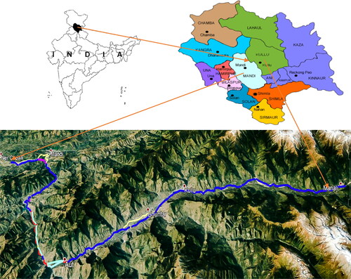
The Ner-Chowk to Manali stretch of National Highway (NH)-21 considered for this study runs through Mandi and Kullu district in the central region of Himachal Pradesh between 77°11'59.308"E 31°46'19.951"N and 77°11'28.124"E 32°14'53.609"N as shown in Figure 1. With a length of about 120 km, this highway stretch passes through the cities of Mandi, Pandoh, Aut, Kullu and Manali. This highway is extremely valuable for socio-economic activities and acts as a feeder to the tourism industry in the region. This highway is also the only source of road connectivity to the Lahul Spiti district, which further connects to the Indo-Pakistan border in Leh district in Jammu and Kashmir. Hence, this highway is of utmost importance from the nation’s socio-economic and strategic defence perspectives. However, the serviceability of this highway is frequently affected by landslides, especially during the monsoon season. Heavy rainfall, ongoing 4 Lanning construction, and complex geo-environmental settings further facilitate the occurrence of landslides in the region.

Figure 1. Location and alignment of highway under study.

2.2. Methodology

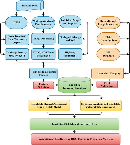
The methodology proposed to carry out the present study incorporates multi-dimensional information acquired from numerous sources to generate the landslide inventory data and the region’s topographical, hydrological, geotechnical, environmental, and anthropological characteristics. These factors were first checked for multicollinearity to identify any correlation between them. The feature selection procedure comprises of the optimum selection of landslide causative factors. These datasets were analyzed using hybrid ML model to produce LSM of the study area. The LSM obtained were classified into five categories and were validated using receiver operating characteristics (ROC) curves and prediction metrics. The ROC curves are well-known techniques to determine the quality of a statistical model by plotting the fraction of true positives values out of total positives values and false positives values out of total negatives values by determining sensitivity and specificity to determine the area under the curve (AUC) values. These curves are indicators of how reliably the areas have been predicted (Vakhshoori and Zare 2018). Further, elements at risk for the highway infrastructure are identified using a deep learning algorithm on a high-resolution LULC map, and the weighted linear combination (WLC) was used to produce the vulnerability map. Finally, the susceptibility and vulnerability maps were integrated to generate the risk map of the highway infrastructure due to landslides. The risk map was further classified into five categories to identify the highway regions that lie in high to very high landslide risk zones. The overall methodology adopted for the present study is summarized through a flow chart as depicted in Figure 2.

Figure 2. Flowchart of methodology for landslide risk analysis.

2.3. Landslide inventory

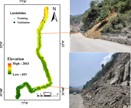
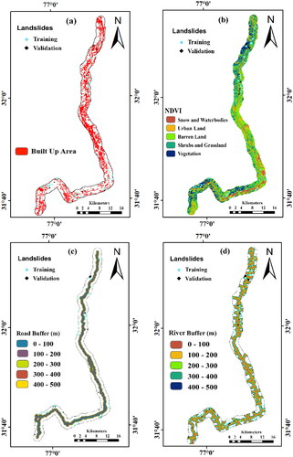
The generation of landslide inventory includes the location of the landslide, damages incurred in terms of life and property, triggering factors, type of landslide and its date and time of occurrence, (Salui 2018; Prakash et al. 2021). In the present study a comprehensive inventory of historical landslides was generated using reports, newspaper articles, Geological Survey of India (GSI), NASA Global Landslide Catalog (GLC), Google earth imagery and was field validated using handheld GPS. The landslide inventory for a highway buffer of 5 km along the alignment was generated. A total of 241 landslide polygons that were identified were further split into training 169 (70%) and 72 (30%) validation dataset as carried out by (Roodposhti et al. 2016; Pham et al. 2019). The maximum and minimum area of landslides was recorded as 2.42x10⁵ m² and 2.1 m^2, respectively as shown in Figure 3. A preliminary investigation of landslide inventory data shows that certain sections of highways were particularly prone to landslides.

Figure 3. Landslide inventory and locations along NH-21.

2.4. Landslide causative factors (LCF)

Identifying and generating landslide causative factors (LCF) is essential for an effective and robust landslide susceptibility model. Several topographical, hydrological, and geological parameters affect the landslide susceptibility of a region, and their selection is generally based on expert options and data availability. The present study incorporates seventeen LCF, which are analyzed for interrelationship using multicollinearity analysis. The Advanced Land Observing Satellite Synthetic Aperture Radar (ALOS PALSAR) 12.5 m digital elevation model generates slope gradient, aspect, plan curvature, elevation, drainage density, distance from rivers, topographic wetness index (TWI), stream power index (SPI) and sediment transport index (STI) maps. Multispectral LANDSAT-8 OLI imagery was used to generate Normalized Difference Vegetation Index (NDVI) and lineament density maps. The geology and lithology maps were procured from the GSI-BHUKOSH portal. The soil map was procured from Bureau of Soil Survey and Land Use Planning (ICAR-NBSS) and digitized in GIS. The state and national highways network present in the study area was procured from the Ministry of Road Transport and Highways (MoRTH) website. The rainfall and temperature data were collected from the Indian Water Portal website and the Indian Meteorological Department (IMD), Shimla and Pune. The high-resolution LULC map of the highway stretch was procured from Himachal Pradesh Council for Science, Technology & Environment (HIMCOSTE). The data obtained from these sources had variable scale and resolution. Hence, the data sources were georeferenced, rasterized, reclassified and resampled to a common raster format of 30 meters.

An optimum selection of LCF's is important for efficient ML modelling process and to reduce the overfitting the model. The selection of these factors also depends upon the data availability and underlying conditions of the study area (Arabameri et al. 2020). Firstly, a multicollinearity test was carried in SPSS software to check the interdependence of LCF's. Any relationship between these factors can decrease the model’s predictability and generate an error in results. In the next step, two feature ranking algorithms chi-squared and random forest feature importance feature ranking algorithms were used to rank LCF's in an ordered manner using a statistical scoring function. The summary of data products and derived information is given in Table 1.

Table 1. Data sources and information derived.

Data	Data Purpose	Data Source	Scale / Resolution
Precipitation Data	Precipitation Characteristics of the Study Area.	https://www.worldclim.org https://weathershimla.nic.in	1:50000
Administrative Reports, Google Earth, (GSI-BHUKOSH)	Historical Landslide Data	https://hpsdma.nic.in/ https://bhukosh.gsi.gov.in/	1:50000
DEM (ALOS-PALSAR)	Curvature, Aspect, Slope, Drainage Density, Elevation, TWI, and SPI	https://search.asf.alaska.edu	12.5 m
Landsat-8 Imagery	LULC, NDVI and Lineament Density	http://earthexplored.usgs.gov	30 m
GSI-BHUKOSH	Lithology, Geology	https://bhukosh.gsi.gov.in/	1:50000
MoRTH	Highway Alignment	https://morth.nic.in/	1:50000
NBSS and LUP	Soil Map	https://www.nbsslup.in/	1:50000
HIMCOSTE	LULC map of the NH-21 stretch	https://himcoste.hp.gov.in/	1:1000

2.5. Certainty Factor (CF) model

The CF is a convenient approach for generating LSM of an area (Kanungo et al. 2011; Devkota et al. 2013). Initially proposed by Buchanan and Shortliffe in 1984, CF model provides a rule-based favourability function to consolidate heterogeneous data layers using Equation (1)(1) $$\mathrm{CF}= \begin{array}{cc}\frac{\mathrm{ }\text{ppa}\mathrm{ }-\mathrm{pps}}{\mathrm{ppa}\left(1-\mathrm{pps}\right)}& \mathrm{ }\text{when}\mathrm{ }\mathrm{ppa}\ge \mathrm{pps}\\ \frac{\mathrm{ppa}-\mathrm{pps}}{\mathrm{pps}\left(1-\mathrm{ppa}\right)}& \mathrm{ }\text{when}\mathrm{ }\mathrm{ppa}<\mathrm{pps}\end{array}$$(1) . (1) $$\mathrm{CF}= \begin{array}{cc}\frac{\mathrm{ }\text{ppa}\mathrm{ }-\mathrm{pps}}{\mathrm{ppa}\left(1-\mathrm{pps}\right)}& \mathrm{ }\text{when}\mathrm{ }\mathrm{ppa}\ge \mathrm{pps}\\ \frac{\mathrm{ppa}-\mathrm{pps}}{\mathrm{pps}\left(1-\mathrm{ppa}\right)}& \mathrm{ }\text{when}\mathrm{ }\mathrm{ppa}<\mathrm{pps}\end{array}$$(1) where CF is the Certainty Factor, ppa is the conditional probability of having a landslide event occurring in class "a", and pps is the prior probability of having the total number of landslides in the study area. The CF value ranges between −1 and +1, where +1 is the measure of belief (definitely true) or increasing certainty of landslide occurrence and −1 is the measure of disbelief (definitely false) or decreasing certainty of landslide occurrence (Zare et al. 2014). The pairwise data layers of all landslides causative factors were combined based on "Z" values obtained from Equation (2)(2) $$\mathrm{Z}=\mathrm{ }\begin{array}{cc}\mathrm{X}+\mathrm{Y}-\mathrm{XY}& X,\mathrm{Y}\ge 0\\ \frac{\mathrm{X}+\mathrm{Y}}{1-\min \hspace{0.17em}\left(\left|X\right|,\left|Y\right|\right)}& \text{X*Y}<0\\ \mathrm{X}+\mathrm{Y}+\mathrm{XY}& X,\mathrm{Y}<0\end{array}$$(2) . (2) $$\mathrm{Z}=\mathrm{ }\begin{array}{cc}\mathrm{X}+\mathrm{Y}-\mathrm{XY}& X,\mathrm{Y}\ge 0\\ \frac{\mathrm{X}+\mathrm{Y}}{1-\min \hspace{0.17em}\left(\left|X\right|,\left|Y\right|\right)}& \text{X*Y}<0\\ \mathrm{X}+\mathrm{Y}+\mathrm{XY}& X,\mathrm{Y}<0\end{array}$$(2)

These pairwise combinations had to be persistently performed on all causative factors using the integration rule until all data layers were combined to prepare final LSM_CF maps using Equation (3)(3) $$\mathrm{LSMCF}=Z_1*\mathrm{CF1}+{ Z}_2\mathrm{*}\mathrm{CF}2+{ Z}_3\mathrm{*}\mathrm{CF}3+\dots +{ Z}_n\mathrm{*}\mathrm{CF}$$(3) . (3) $$\mathrm{LSMCF}=Z_1*\mathrm{CF1}+{ Z}_2\mathrm{*}\mathrm{CF}2+{ Z}_3\mathrm{*}\mathrm{CF}3+\dots +{ Z}_n\mathrm{*}\mathrm{CF}$$(3)

2.6. Random Forest (RF) model

The RF model is an ensemble model that uses a decision tree (DT) supervised classification algorithm and combines multiple trees and branches with random data. (Breiman 2001; Arabameri et al. 2019). Bootstrapping or bagging is the process of sampling by decorrelating the trees to reduce the noise in a single training set. This technique decreases the variance and leads to better model performance. The out-of-bag (OBB) error is used to calculate variable importance and validate RF model (Merghadi et al. 2020). The OBB error estimates the B(x) value over a vector X and can be expressed using Equation (4)(4) $$B{\left(X\right)}^{\mathit{OBB}}=\mathit{argmax}\sum _{t=1}^T{\Vert (b}_t\left(X\right)=y).\Vert (X{∊H}_T)$$(4) . The Gini impurity index measures the probability of incorrectly classified randomly selected variables and is used for determining the split in trees (Sahin et al. 2020). The mean Gini index is derived using Equation (5)(5) $$\text{Ginni Impurity}=1-\sum _{i=1}^{\mathrm{n}}{\left(P_i\right)}^2$$(5) . The features having lowest value are preferred. (4) $$B{\left(X\right)}^{\mathit{OBB}}=\mathit{argmax}\sum _{t=1}^T{\Vert (b}_t\left(X\right)=y).\Vert (X{∊H}_T)$$(4) where $X$ is the vector variable, $y$ is output space, $H_T$ represents number of base learners from 1 to $t$ and $\Vert$ is the if else indicator function. (5) $$\text{Ginni Impurity}=1-\sum _{i=1}^{\mathrm{n}}{\left(P_i\right)}^2$$(5) where $P_i$ is the probability of a sample being classified to a particular class $\mathrm{n}$

A robust RF model requires tuning of hyper-parameters such as (i) number of combined trees (ntree), (iii) maximum features considered at every split (mtree) and (iv terminal node size (nodesize) (Fang et al. 2020; Pourghasemi et al. 2020).

2.7. U-net deep learning network

A U-net network consists of a U-shaped structure that is conventionally designed for biomedical image segmentation to obtain circumstantial and location information simultaneously (Soares et al. 2020). U-net is extensively used in image analysis and segmentation where the inputs and outputs have similar spatial resolution, thereby establishing a cascade of connections during the up-sampling process. The deep learning framework of U-net can distinguish and localize borders precisely by performing classification on every pixel so that the input and output share the same size. The U-net model training requires a number of annotated images and uses data augmentation with elastic deformations and obtains context and location information simultaneously (Li et al. 2021). The structure of a U-net consists of an encoder that extracts and reduces the spatial dimensions in every layer from images and divides the image into different scales and a decoder that increases the spatial dimensions.

3. Analysis of results

3.1. Multicollinearity analysis and optimum feature selection

Selecting a relevant subset of landslide causative factors (LCF) is paramount for generating an efficient and robust landslide risk model and minimizing the interdependence of variables. In the first step the independent variables were analyzed for any corelation using a multicollinearity test. The tolerance (TOL) and Variance Inflation Factor (VIF) parameters are utilized to analyze the multicollinearity among independent variables. Generally, VIF values < 10 and TOL values > 0.1 are acceptable for no multicollinearity among variables. The results of multicollinearity analysis were presented in Table 2. The results indicated no problem of multicollinearity among the selected 17 independent variables.

Table 2. Results of multicollinearity analysis.

Landslide Causative Factors	Collinearity Statistics
	Tolerance	VIF
Slope Aspect	0.698	2.451
Slope Gradient	0.775	1.165
STI	0.286	2.544
Plan Curvature	0.614	8.793
SPI	0.449	5.489
Elevation	0.531	3.037
Distance from rivers	0.486	4.785
Drainage Density	0.612	8.525
LULC	0.489	6.785
Rainfall	0.725	7.354
Geology	0.196	2.976
Lithology	0.825	1.215
NDVI	0.201	7.631
Lineament Density	0.792	5.270
Distance from Roads	0.257	7.638
Soil	0.312	3.365
TWI	0.402	4.686

In the next step two statistical feature ranking methods, i.e. chi-squared and random forest feature importance tests, were used to rank the independent variables. The output produced by the two ranking algorithms indicates that each method has different feature weights and orders Table 3. The results based on expert opinions and various field surveys, a cut off value of 50% was selected for which 9 factors were deemed to be most influential for landslide occurrence and were used for further analysis.

Table 3. Output of feature ranking algorithms.

Chi-Squared		Random Forest Feature Importance
Rainfall	0.577	Distance to Roads	124.96
Elevation	0.545	TWI	111.94
Distance to Roads	0.499	Rainfall	105.32
Drainage Density	0.420	Drainage Density	102.68
TWI	0.391	Distance to Rivers	94.72
Slope Gradient	0.365	Slope Gradient	81.64
Geology	0.329	Elevation	70.61
Distance to Rivers	0.302	NDVI	69.33
NDVI	0.287	Geology	65.73
Plan Curvature	0.136	STI	61.35
Soil	0.098	SPI	69.88
Slope Aspect	0.089	Lineament Density	52.73
LULC	0.805	LULC	45.25
Lineament Density	0.075	Soil	33.35
STI	0.045	Slope Aspect	24.65
SPI	0.023	Lithology	9.15
Lithology	0.015	Plan Curvature	7.149

3.2. Landslide hazard analysis

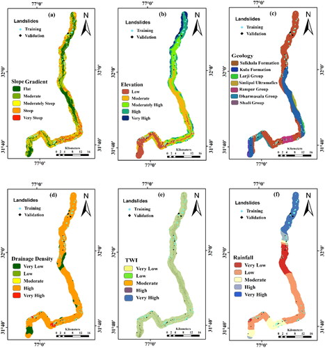
The drainage density, TWI, geology, elevation and slope gradient, which were the major contributing LCF in feature selection were selected for hazard analysis as depicted in Figure 4. The LCF maps indicate that the elevation increases from 693 m in the southern to 2843 m towards the northern region of the highway. The slope of the highway stretch is generally moderate but tends to be high in the southern region. Geologically, the region consists of Salkhala and Kullu formations, both of which have erosion-prone characteristics. As the majority of the highway stretch runs along river Beas, regions with high drainage density and TWI are present in the highway stretch.

Figure 4. LCF for NH-21 stretch (a) Slope Gradient (b) Elevation (c) Geology (d) Drainage Density (e) TWI and (f) Rainfall.

A hybrid CF-RF model was generated for landslide susceptibility analysis. The CF values obtained were used to analyze the contribution of individual LCF classes, and the relative contribution of each LCF was made through Gini impurity index values. The LCF were reclassified using the CF values. The reclassified LCF were then used as an RF model input and a 10 k-fold landslide training dataset. The CF values and Gini impurity index (GI) are shown in Table 4. The final LSM map was classified into very low, low, moderate, high and very high susceptibility classes.

Table 4. CF values of classes and gini impurity index for LCF obtained from CF-RF model.

LCF	Class Pixels	Percent of Pixels	Landslide Pixels	Percent of Pixels	Certainty Factor	Random Forest
					CF Value	Gini Impurity
Slope Gradient (Degree)
Flat (<15°)	521169	0.252	328	0.284	−0.128	458.47
Moderate (15° − 25°)	443364	0.214	245	0.212	0.991
Moderately Steep (25° − 35°)	499527	0.241	259	0.224	0.991
Steep (35° − 45°)	430798	0.208	257	0.222	0.948
Very Steep (>45°)	176411	0.085	67	0.058	0.752
Elevation (m)
Low (400 - 1000)	393024	0.190	42	0.036	0.525	239.82
Moderate (1000 − 1500)	657705	0.318	26	0.022	0.424
Moderately High (1500 − 2000)	507897	0.245	442	0.382	0.827
High (2000 − 2500)	378391	0.183	616	0.533	−0.727
Very High (2500 − 3500)	134252	0.065	30	0.026	−0.562
Drainage Density
Very Low (0 − 0.6)	212186	0.102	89	0.077	−0.561	689.56
Low (0.6 − 1.2)	652865	0.315	73	0.063	−0.543
Moderate (1.2 − 1.8)	857389	0.414	593	0.513	0.316
High (1.8 − 2.4)	214676	0.104	345	0.298	0.477
Very High (2.4 − 3.0)	134153	0.065	56	0.048	0.733
Geology
Larji Group	88325	0.067	42	0.036	0.408	464.89
Shali Group	97377	0.086	126	0.109	−0.455
Salkhala Formation	646414	0.457	369	0.319	0.525
Kullu Formation	316565	0.056	257	0.222	0.326
Simplipal Ultramafic	167318	0.081	130	0.112	0.197
Rampur Group	118914	0.057	89	0.077	−0.536
TWI
Very Low (0.00 − 4.00)	638201	0.308	366	0.317	−0.166	384.27
Low (4.00 − 10.00)	936230	0.452	550	0.476	−0.194
Moderate (10.00 − 16.00)	383547	0.185	163	0.141	0.150
High (16.00 − 22.00)	99116	0.048	57	0.049	0.168
Very High (22.00 − 28.00)	14175	0.007	20	0.017	0.542

The ROC curves are shown in Figure 5, and the values of prediction matrices are given in Table 5. The results indicate that the model had excellent predictive potential with AUC values of (0.939, 0.941), accuracy (0.928) and kappa (0.644). The computational errors indicate that the model has minimal MAE (0.168) and RMSE (0.317) errors.

Figure 5. ROC curves and AUC values for CF-RF model.

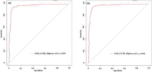
Table 5. Prediction matrices for CF-RF model.

Model	AUCPr	AUCVal	Accuracy	Precision	MAE	RMSE	F1	Kappa	Recall
CF-RF	0.939	0.941	0.928	0.923	0.168	0.317	0.825	0.644	0.837

The temporal probability of landslides was calculated by multiplication of rainfall map with annual exceedance probability. The annual exceedance is the probability of rainfall exceeding a specific threshold value in a given year. Due to the study area’s unavailability of temporal landslide event data, the annual rainfall was plotted against the logarithmic scale return period. The threshold values were obtained for a five-year return period, as shown in Figure 6. The five-year return period was calculated for 110 cm of rainfall, and the temporal probability rainfall map was prepared by taking this value as maximum threshold rainfall. The study area was divided into low, low, moderate, high and very high probabilities. The final landslide hazard map was prepared using multiplying spatial and temporal probabilities and classified into five zones along with percentage of area in each zone, as shown in Figure 7(a).

Figure 6. Annual exceedance rainfall and return period.

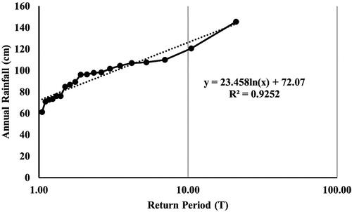
Figure 7. Landslide maps and percentage of area (a) LHM (b) LVM (c) LRM.

3.3. Landslide vulnerability analysis and elements at risk

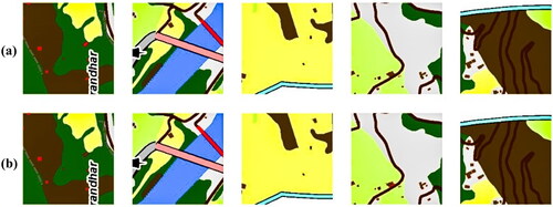
The present study incorporates the built-up area as the major element at risk as such areas have a major concentration of population due to residential or commercial purposes. Such buildings often include slope excavation works resulting in slope instability leading to landslides in their vicinity. The built-up area was extracted from high-resolution imagery using a U-Net deep learning algorithm to delineate the built-up area polygons. The method used for training the mirror image is the rotation of the original image. The output image contains an original built-up area image and a mirror image for the batter training dataset. Separate paths were used for reading ground truth and training image with the proportion of training set: test set: verification set as 8:1:1, with uniform sampling as shown in Figure 8. The training and validation loss of the U-Net deep learning algorithm, along with the number of batches processed, is shown in Figure 9.

Figure 8. Built-up area extraction using U-net (a) Ground Truth (b) Predictions.

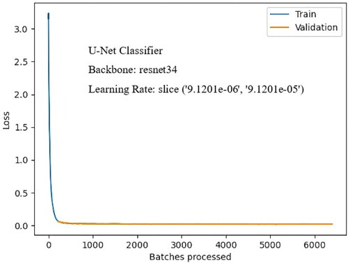
Figure 9. Training and validation loss of U-net model.

Initially, the pixel accuracy of the U-net network model is low and showed high growth after the 200^th epoch. The graph shows minimal fluctuation and indicates that the model is stable. The prediction matrices of the U-Net model are shown in Table 6. The U-Net classifier was able to identify 43,972 polygons of built-up area with an archived classification accuracy of 96.4% in the training data set, and the loss rate of the model training is 0.07 per cent which is comparatively very low.

Table 6. Predictive performance of U-net model.

U-Net	Accuracy	Precision	Recall
Built-Up	0.964	0.958	0.955
No Data	0.994	0.996	0.995

A detailed analysis of vulnerability should take into account the several parameters to spatially estimate the potential to social or economic damage. The landslide vulnerability map of the study area was prepared by the weighted linear combination method (WLC) by assigning relative weights to NDVI, road buffer, river buffer and built-up areas in the GIS environment Figure 10. The weights assigned were based on expert opinions, logical progressions and field observations e.g. the built-up areas are the commercial and residential zones that are prone to landslides and were given maximum weightage. Similarly, the road network which serves as a lifeline for communities living in mountainous regions is given higher priority. The agricultural area and the dwellings along the drainage networks were also considered to be relevant vulnerable spots for landslides. The final vulnerability map was prepared using Equation (6)(6) $$\text{LVM}=\mathrm{(}\text{Built}\mathrm{ }-\mathrm{ }\text{Area}\mathrm{)}*0.3+\mathrm{(}\text{NDVI}\mathrm{)}*0.2+\mathrm{(}\text{Road}\mathrm{ }\text{Buffer}\mathrm{)}*0.3\mathrm{ }+\mathrm{(}\text{River}\mathrm{ }\text{Buffer}\mathrm{)}*0.2$$(6) . (6) $$\text{LVM}=\mathrm{(}\text{Built}\mathrm{ }-\mathrm{ }\text{Area}\mathrm{)}*0.3+\mathrm{(}\text{NDVI}\mathrm{)}*0.2+\mathrm{(}\text{Road}\mathrm{ }\text{Buffer}\mathrm{)}*0.3\mathrm{ }+\mathrm{(}\text{River}\mathrm{ }\text{Buffer}\mathrm{)}*0.2$$(6)

Figure 10. Landslide vulnerability factors (a) Built-Up Area (b) NDVI (c) Distance from Road (d) Distance from Rivers.

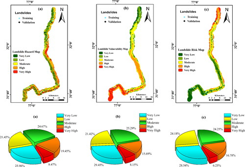
The vulnerability was classified into five categories i.e. very low, low, moderate, high and very high vulnerability. The analysis of the vulnerability map indicates that 15.69% and 8.15% of the total area falls into high to very high vulnerability zone, respectively, as shown in Figure 7(b).

3.4. Landslide risk analysis

The landslide risk in the present study is correlated to damages that might incur in terms of loss of buildings and road infrastructure in a 5 km highway buffer zone. The landslide risk map (LRM) was generated by the multiplication of landslide hazard and vulnerability maps. The landslide risk map was classified into five zones of very low, low, moderate, high and very high-risk zones. The analysis of the risk map indicates that 16.78% and 6.25% of the total area along the 5 km buffer zone of highway alignment is under high and very high landslide risk, respectively as shown in Figure 7(c).

4. Discussion

The stretch NH-21 chosen for the present study faces numerous landslide events, especially during peak monsoon season, due to its complex geo-environmental settings and ongoing 4-lanning construction activities. The landslide inventory for a highway buffer of 5 km along the alignment is generated with 241 landslide polygons. Creating a geospatial landslide inventory of the study area is essential for landslide risk assessment and management by collating information from various sources. The analysis of the LSM using CF-RF model depicted higher predictive potential than similar studies done using individual models by (Zare et al. 2014; Goetz et al. 2015; Bui et al. 2020). This shows that the hybrid integration of such models is beneficial for building a robust model. The model indicated that 19.45% and 8.47% of the highway study area falls in high and very high susceptibility zones, respectively. The highest GI values were obtained for drainage density (689.56), followed by geology (464.89) and slope gradient (458.47), showing a greater correlation to landslide occurrence. The CF values obtained suggest that very high drainage density (0.733) coupled with moderate (0.991) to steep slopes (0.948), especially in the geological regions of Shankhala formation (0.525), are particularly susceptible to landslides. The results show that 8.5% of the study area comes under very high hazard zone especially in the central regions of highway alignment near the Hanogi temple and Aut tunnel regions where extensive slope excavation is being carried out for highway construction. Along the highway alignment, the southern and north-western regions come under low to medium-hazard zones. The hazard map could provide useful information to the development authorities to carry out regional landslide prevention activities. The vulnerability map depicts that the southern and north-eastern regions along the highway alignment, including the location of populated cities like Mandi and Kullu, are particularly vulnerable to landslides. Such information could be very useful to the stakeholders in planning construction activities in the region. The areas near the vicinity of roads having high drainage density were found to be at greater risks. The infrastructure near such areas should have greater impact from a landslide event in the future. In comparison to similar studies to carry out a landslide risk analysis of similar regions (Batista et al. 2019; Dikshit et al. 2020; Mallick et al. 2021), this study was able to predict the landslide risk, spatially with higher accuracy and was able to prcisely identify the elements at risk using deep learning based models. Such a study will provide valuable information to the government authorities about the landslide risk posed to the population and help implement timely mitigation measures.

5. Conclusion

Over the past few decades, the Himalayan region has witnessed a particular increase in landslide events due to climate change and increasing human interference with the environment. Hence, there is a need to constantly evaluate the risk posed to human lives and infrastructure in such regions due to landslide events. This study has generated a landslide risk map for a stretch of NH-21 from Ner-Chowk to Manali which is an important from economic and defence perspective. The methodology of accessing landslide risk is based on the spatial multiplication of landslide hazard and vulnerability. The optimum feature selection is a crucial component in landslide analysis as it increases the prediction capability and minimizes the computational requirements of the model. The landslide hazard map is compiled by determining the spatial and temporal landslide probabilities. The spatial probability (susceptibility) map was prepared using the CF-RF hybrid model. The temporal probability was calculated using the annual exceedance rainfall threshold for the five-year return period. The elements at risk were delineated using a deep learning U-Net framework to identify the built-up areas from a high-resolution LULC map. The deep learning framework is an efficient way of delineating objects by image analysis. The framework is both efficient and time-saving but has high computational requirements. The vulnerability map was prepared using WLC method based on expert opinions and extensive field surveys. The final risk map was classified into five risk zones to determine the areas under high and very high landslide risk. The spatial risk analysis of the NH-21 highway stretch puts 16.78% and 6.25% area under high and very high landslide risk zones, respectively. Such areas should be carefully inspected before any construction planning activities, and adequate warning and mitigation measures should be implemented for the effective functioning of the highway. However, these maps can further be modified by incorporating more detailed data like landslide type, disruption to highway serviceability and population diversity etc. A major hindrance while analyzing the landslide risk in such regions is the lack of precise temporal data records of landslides, rainfall and a true measure of disruptions to the elements at risk. Therefore, a detailed risk analysis of landslides could be carried out by collecting the actual economic damage and social loss due to landslides on a temporal scale for developing a deeper understanding of landslide risk on a regional scale.

Disclosure statement

No potential conflict of interest was reported by the authors.

References

- Achour Y, Boumezbeur A, Hadji R, Chouabbi A, Cavaleiro V, Bendaoud EA. 2017. Landslide susceptibility mapping using analytic hierarchy process and information value methods along a highway road section in Constantine, Algeria. Arab J Geosci. 10(8):1–16.
- Arabameri A, Karimi-Sangchini E, Pal SC, Saha A, Chowdhuri I, Lee S, Bui DT. 2020. Novel credal decision tree-based ensemble approaches for predicting the landslide susceptibility. Remote Sens. 12(20):3389. [accessed 2021 July 26].
- Arabameri A, Pradhan B, Rezaei K, Lee C-WW. 2019. Assessment of landslide susceptibility using statistical- and artificial intelligence-based FR-RF integrated model and multiresolution DEMs. Remote Sens [Internet]. 11(9):999. [accessed 2021 July 31].
- Azimi SR, Nikraz H, Yazdani-Chamzini A. 2018. Landslide risk assessment by using a new combination model based on a fuzzy inference system method. KSCE J Civ Eng. 22(11):4263–4271. [accessed 2021 December 29]. www.springer.com/12205.
- Batista EF, Passini LDB, Kormann ACM. 2019. Methodologies of economic measurement and vulnerability assessment for application in landslide risk analysis in a highway domain strip: a case study in the Serra Pelada Region (Brazil). Sustain 11(21):6130. [accessed 2022 January 3].
- Breiman L. 2001. Random forests. Mach Learn. 45(1):5–32.
- Bui DT, Tsangaratos P, Nguyen VT, Liem NV, Trinh PT. 2020. Comparing the prediction performance of a Deep Learning Neural Network model with conventional machine learning models in landslide susceptibility assessment. Catena [Internet]. 188(July 2019):104426.
- Castellanos Abella EA, Van Westen CJ. 2008. Qualitative landslide hazard and risk assessment using multicriteria analysis; a case study from San Antonio del Sur, Guantánamo, Cuba. Geomorphology 94(3–4):453–466.
- Chen W, Xie X, Peng J, Shahabi H, Hong H, Bui DT, Duan Z, Li S, Zhu A-X. 2018. GIS-based landslide susceptibility evaluation using a novel hybrid integration approach of bivariate statistical based 2 random forest method [Internet]. [accessed 2021 July 31]. http://www.elsevier.com/open-access/userlicense/1.0/2.
- Chen W, Fan L, Li C, Pham BT. 2019. Spatial prediction of landslides using hybrid integration of artificial intelligence algorithms with frequency ratio and index of entropy in Nanzheng County, China. Appl Sci 2020. 10(1):29. [accessed 2021 July 31].
- Chen W, Pourghasemi HR, Naghibi SA. 2018. A comparative study of landslide susceptibility maps produced using support vector machine with different kernel functions and entropy data mining models in China. Bull Eng Geol Environ. 77(2):647–664.
- Chun Z, Shihui P, Junzheng Z, Zhigang T, Wenshuai H, Xuehan Y. 2019. Analysis of slope deformation caused by subsidence of goaf on tonglushan ancient mine relics. Geotech Geol Eng. 37(4):2861–2871.
- Dai FC, Lee CF, Ngai YY. 2002. Landslide risk assessment and management: an overview. Eng Geol. 64(1):65–87.
- Devkota KC, Regmi AD, Pourghasemi HR, Yoshida K, Pradhan B, Ryu IC, Dhital MR, Althuwaynee OF. 2013. Landslide susceptibility mapping using certainty factor, index of entropy and logistic regression models in GIS and their comparison at Mugling-Narayanghat road section in Nepal Himalaya. Nat Hazards. 65(1):135–165.
- Dikshit A, Sarkar R, Pradhan B, Acharya S, Alamri AM. 2020. Spatial landslide risk assessment at Phuentsholing, Bhutan. Geosci. 10(4):131. [accessed 2022 February 10].
- Dou J, Bui DT, Yunus AP, Jia K, Song X, Revhaug I, Xia H, Zhu Z. 2015. Optimization of causative factors for landslide susceptibility evaluation using remote sensing and GIS data in parts of Niigata, Japan. PLoS One. 10(7):e0133262. [accessed 2021 July 31].
- Fang Z, Wang Y, Peng L, Hong H. 2020. Integration of convolutional neural network and conventional machine learning classifiers for landslide susceptibility mapping. Comput Geosci. 139:104470.
- Fell R. 1993. Landslide risk assessment and acceptable risk. (4). Canadian Geotech J. 31(2): 261–272.
- Ghosh T, Bhowmik S, Jaiswal P, Ghosh S, Kumar D. 2020. Generating substantially complete landslide inventory using multiple data sources: a case study in Northwest Himalayas, India. J Geol Soc India. 95(1):45–58. [accessed 2021 July 31].
- Goetz JN, Brenning A, Petschko H, Leopold P. 2015. Evaluating machine learning and statistical prediction techniques for landslide susceptibility modeling. Comput Geosci. 81:1–11.
- Kanungo DP, Sarkar S, Sharma S, Sarkar ÁS, Sharma ÁS, Sarkar S, Sharma S. 2011. Combining neural network with fuzzy, certainty factor and likelihood ratio concepts for spatial prediction of landslides. Nat Hazards. 59:1491–1512.
- Kutlug Sahin E, Ipbuker C, Kavzoglu T. 2017. Investigation of automatic feature weighting methods (Fisher, Chi-square and Relief-F) for landslide susceptibility mapping. Geocarto Int. 32(9):956–977.
- Lallianthanga RK, Lalbiakmawia F, Lalramchuana F. 2013. Landslide hazard zonation of Mamit Town, Mizoram, India using remote sensing and GIS techniques. Int J Geol Earth Environ Sci. 3(1):184–194.
- Lee S, Talib JA. 2005. Probabilistic landslide susceptibility and factor effect analysis. Environ Geol. 47(7):982–990. [accessed 2021 August 5].
- Li L, Qin Z, Zhang Q. 2021. Landslide recognition based on the improved U-net. In Proceedings of the 4th International Conference on Computer Science and Software Engineering (CSSE '21). Association for Computing Machinery, New York, NY, USA, 338–345.
- Li ZH, Huang HW, Xue YD, Yin J. 2009. Risk assessment of rockfall hazards on highways. Georisk. 3(3):147–154.
- Luo X, Lin F, Chen Y, Zhu S, Xu Z, Huo Z, Yu M, Peng J. 2019. Coupling logistic model tree and random subspace to predict the landslide susceptibility areas with considering the uncertainty of environmental features. Sci Reports. 9(1):1–13. [accessed 2021 August 23].
- Mallick J, Alqadhi S, Talukdar S, Alsubih M, Ahmed M, Khan RA, Kahla NB, Abutayeh SM. 2021. Risk assessment of resources exposed to rainfall induced landslide with the development of GIS and RS based ensemble metaheuristic machine learning algorithms. Sustain. 13(2):457. [accessed 2021 December 29].
- Mattsson LG, Jenelius E. 2015. Vulnerability and resilience of transport systems - A discussion of recent research. Transp Res Part A Policy Pract. 81:16–34.
- Merghadi A, Yunus AP, Dou J, Whiteley J, ThaiPham B, Bui DT, Avtar R, Abderrahmane B. 2020. Machine learning methods for landslide susceptibility studies: a comparative overview of algorithm performance. Earth-Science Rev. 207:103225.
- Monsieurs E, Dewitte O, Demoulin A. 2019. A susceptibility-based rainfall threshold approach for landslide occurrence. Nat Hazards Earth Syst Sci. 19(4):775–789.
- Nguyen H-D, Pham V-D, Nguyen Q-H, Pham V-M, Pham MH, Vu VM, Bui Q-T. 2020. An optimal search for neural network parameters using the Salp swarm optimization algorithm: a landslide application. Remote Sens Lett. 11(4):353–362. [accessed 2021 August 5]. https://doi.org/10.1080/2150704X.2020.1716409.
- Nohani E, Moharrami M, Sharafi S, Khosravi K, Pradhan B, Pham BT, Lee S, Melesse AM. 2019. Landslide susceptibility mapping using different GIS-Based bivariate models. Water (Switzerland). 11(7):1402–1424.
- Ozioko OH, Igwe O. 2020. GIS-based landslide susceptibility mapping using heuristic and bivariate statistical methods for Iva Valley and environs Southeast Nigeria. Environ Monit Assess [Internet]. 192(2):119–133 [accessed 2021 August 5].
- Pham BT, Shirzadi A, Shahabi H, Omidvar E, Singh SK, Sahana M, Asl DT, Ahmad BB, Quoc NK, Lee S. 2019. Landslide susceptibility assessment by novel hybrid machine learning algorithms. Sustain. 11(16):1–25.
- Pham BT, Tien Bui D, Prakash I, Dholakia MB. 2016. Rotation forest fuzzy rule-based classifier ensemble for spatial prediction of landslides using GIS. Nat Hazards. 83(1):97–127.
- Pourghasemi HR, Kariminejad N, Amiri M, Edalat M, Zarafshar M, Blaschke T, Cerda A. 2020. Assessing and mapping multi-hazard risk susceptibility using a machine learning technique. Sci Rep. 10(1):1–11. [accessed 2021 November 16].
- Pradhan SP, Siddique T. 2020. Stability assessment of landslide-prone road cut rock slopes in Himalayan terrain: A finite element method based approach. J Rock Mech Geotech Eng. 12(1):59–73.
- Prakash N, Manconi A, Loew S. 2021. A new strategy to map landslides with a generalized convolutional neural network. Sci Reports. 11(1):1–15. [accessed 2021 November 16].
- Roodposhti MS, Aryal J, Shahabi H, Safarrad T. 2016. Fuzzy Shannon entropy: A hybrid GIS-based landslide susceptibility mapping method. Entropy. 18(10):343. [accessed 2021 September 16].
- Saha S, Arabameri A, Saha A, Blaschke T, Ngo PTT, Nhu VH, Band SS. 2021. Prediction of landslide susceptibility in Rudraprayag, India using novel ensemble of conditional probability and boosted regression tree-based on cross-validation method. Sci Total Environ. 764:142928.
- Sahin EK, Colkesen I, Acmali SS, Akgun A, Aydinoglu AC. 2020. Developing comprehensive geocomputation tools for landslide susceptibility mapping: LSM tool pack. Comput Geosci. 144:104592.
- Sahin EK. 2020. Comparative analysis of gradient boosting algorithms for landslide susceptibility mapping. Geocarto Int. 37:2441–2465. [accessed 2021 December 5]. https://doi.org/10.1080/10106049.2020.1831623.
- Salui CL. 2018. Methodological validation for automated lineament extraction by LINE method in PCI geomatica and MATLAB based Hough transformation. J Geol Soc India. 92(3):321–328. [accessed 2021 July 31].
- Sharma A, Prakash C, Manivasagam VS. 2021. Entropy-based hybrid integration of random forest and support vector machine for landslide susceptibility analysis. Geomatics. 1(4):399–416. [accessed 2021 December 3].
- Sharma A, Prakash C, Sharma A, Sharma P. 2022. Hybrid machine learning and optimum feature selection based landslide susceptibility analysis inventory of glaciers and evolution of glacial lake changes using remote sensing techniques in Himachal Pradesh view project hybrid machine learning and optimum feature selection based landslide susceptibility analysis. Artic Int J Geoinformatics. 18(3):67–87. [accessed 2022 October 16]. https://www.researchgate.net/publication/361310466.
- Sharma A, Prakash C. 2022. Predicting landslide susceptibility of a mountainous region using a hybrid machine learning-based model. In: Ashish, D.K., de Brito, J. editors. Environmental Concerns and Remediation. Cham: Springer. [accessed 2022 October 16].
- Soares LP, Dias HC, Grohmann CH. 2020. Landslide segmentation with U-net: evaluating different sampling methods and patch sizes. ArXiv [accessed 2022 April 19].
- Song S, Zhao M, Zhu C, Wang F, Cao C, Li H, Ma M. 2022. Identification of the potential critical slip surface for fractured rock slope using the Floyd algorithm. Remote Sens. 14(5):1284. [accessed 2023 January 21].
- Sufi FK, Alsulami M. 2021. Knowledge discovery of global landslides using automated machine learning algorithms. IEEE Access. 9:131400–131419.
- Sufi FK. 2021. AI-Landslide: software for acquiring hidden insights from global landslide data using artificial intelligence. Softw Impacts. 10:100177.
- Vakhshoori V, Zare M. 2018. Is the ROC curve a reliable tool to compare the validity of landslide susceptibility maps? Geomatics, Nat Hazards Risk. 9(1):249–266. [accessed 2023 January 20]. http://www.tandfonline.com/action/journalInformation?show=aimsScope&journalCode=tgnh20#VsXodSCLRhE.
- Versain LD. 2019. Bi-variate statistical approach in landslide hazard zonation: central Himalayas of Himachal Pradesh, India. Int J Appl Eng Res. 14(2):415–428.
- Vulnerability S, Risk Assessment. 2015. Preparation of Hazard, Vulnerability & Risk Analysis atlas and report for the state of Himachal Pradesh. (March).
- Wang H, Zhang L, Yin K, Luo H, Li J. 2021. Landslide identification using machine learning. Geosci Front. 12(1):351–364.
- Wang L-J, Guo M, Sawada K, Lin J, Zhang J, Wang L-J, Guo M, Sawada K, Lin J, Zhang J. 2016. A comparative study of landslide susceptibility maps using logistic regression, frequency ratio, decision tree, weights of evidence and artificial neural network. GescJ. 20(1):117–136. [accessed 2021 August 5].
- Yang J, Sun H, Wang L, Li L, Wu B. 2013. Vulnerability evaluation of the highway transportation system against meteorological disasters. Procedia - Soc Behav Sci. 96(Cictp):280–293.
- Yi Y, Zhang Z, Zhang W, Xu Q, Deng C, Li Q. 2019. GIS-based earthquake-triggered-landslide susceptibility mapping with an integrated weighted index model in Jiuzhaigou region of Sichuan Province, China. Nat Hazards Earth Syst Sci. 19(9):1973–1988.
- Zare M, Jouri MH, Salarian T, Askarizadeh D. 2014. Comparing of bivariate statistic, AHP and combination methods to predict the landslide hazard in northern aspect of Alborz Mt. (Iran). Int J Agric Crop Sci:7:543–554.
- Zhang X, Zhu C, He M, Dong M, Zhang G, Zhang F. 2021. Failure mechanism and long short-term memory neural network model for landslide risk prediction. Remote Sens. 14(1):166. [accessed 2023 January 21].