Estimation of grassland aboveground biomass combining optimal derivative and raw reflectance vegetation indices at peak productive growth stage

Abstract

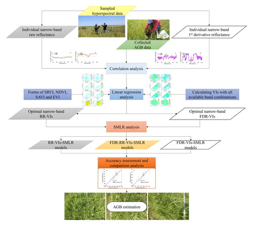
In this paper, field spectroradiometer and aboveground biomass (AGB) data were acquired at the harvest stage at two sites in semiarid grasslands in Inner Mongolia, China. Four forms of commonly used vegetation indices (VIs) using all possible combinations of narrow-band first derivative (FDR) and raw reflectance (RR) were calculated, and the best FDR-VIs and RR-VIs were chosen by a linear regression analysis against AGB. The stepwise multiple linear regression (SMLR) models using the optimal FDR-VIs, RR-VIs, and both FDR-VIs and RR-VIs as input variables were developed for estimating the AGB. Results demonstrated that the estimation performance using the best FDR-VIs were comparable with the best RR-VIs, while the accuracy has been further improved by combining the best FDR-VIs and RR-VIs (maximum decrease in RMSE of 44% and minimum RMAE of 4.7%). The approach was found to be an important step for more accurate and effective grassland AGB estimation.

Graphical Abstract

Keywords:

• Grassland aboveground biomass
• derivative spectral analysis
• hyperspectral vegetation indices
• stepwise multiple regression model
• field experiments

1. Introduction

Grasslands are one of the most important natural ecosystems for human beings and have diverse functions (Wang et al. 2022). They not only occupy the majority of the global agricultural lands, but also play indispensable roles in ecosystems service and livestock production systems on all continents (Li et al. 2015). Quantification of the grassland aboveground biomass (AGB), an indicator of the forage yield, is critical in understanding grassland productivity for animal grazing, evaluating livestock carrying capacity, providing improved management of rangeland resources, and achieving sustainable development (Kumar and Mutanga 2017; Schucknecht et al. 2017; He et al. 2019; Bayaraa et al. 2021). Though the conventional “mow-dry-and-weigh” approaches of measuring AGB are accurate, they are destructive, costly, labor-intensive, time-consuming and it is difficult to obtain real-time AGB properties (Barrachina et al. 2015; Li et al. 2017; Bretas et al. 2021; Zhang et al. 2021). Alternatively, hyperspectral remote sensing techniques, which can collect dozens or hundreds of narrow spectral bands, are known as a nondestructive and cost-effective way and have exhibited the capability to measure vegetation variables. Ground-based and airborne hyperspectral systems have been used as a rapid and non-destructive method to obtain the variability of AGB, and to deepen our understanding of plant characteristics as well as nutritional status in both agricultural and environmental ecosystems (Fricke and Wachendorf 2013; Mahajan et al. 2017; Moeckel et al. 2017; Xu et al. 2017; Eon et al. 2019; Singh et al. 2022).

Vegetation indices (VIs) are linear or nonlinear combinations of different sensitive spectral bands, which can reflect more additional implicit information than a single spectral band (Chen et al. 2009). Statistical approaches and hyperspectral VIs have been widely adopted to accurately and efficiently characterize plant biomass, leaf area index, and grain yield within different agricultural applications (Fava et al. 2009; Foster et al. 2017; Tao et al. 2020; Costa et al. 2021; Zhang et al. 2021). Moreover, estimation of grassland AGB by hyperspectral remote sensing is usually done by using the unique spectral reflectance characteristics of green vegetation, selecting different raw or derivative reflectance bands to construct suitable VIs, and then employing the VIs to build models to estimate the AGB. Most VIs only use spectral reflectance information from two fixed wavelength ranges of visible and near-infrared (NIR), i.e. by comparing the strong absorption in the red bands caused by chlorophyll with high reflection in the near-infrared bands caused by multiple scattering. Even so, accurate and rapid estimation of AGB is still a challenging task for hyperspectral remote sensing studies, particularly in a high vegetation cover (VC) or leaf area index (LAI) period (Luo et al. 2017a). One main obstacle is saturation in the estimation, and this problem is characterized by the lower sensitivity of VIs calculated from the red and NIR reflectance in the presence of dense canopy. That is, high biomass and LAI is obtained, due to the red and NIR reflectance asymptotically approaching a saturation level (Gao et al. 2000).

Several studies have been conducted to prove the feasibility of the optimal delineation of grassland AGB using hyperspectral measurements in recent decades (Boschetti et al. 2007; Fava et al. 2009; Fava et al. 2010; Foster et al. 2017; Luo et al. 2017b; Moeckel et al. 2017; Obermeier et al. 2019). The application of narrow-band VIs derived from hyperspectral data can provide additional and implicit information, and reduce the influences of atmospheric and water absorption, soil background, and the saturation problem of broadband VIs (Chen et al. 2009; Gnyp et al. 2014a; Zandler et al. 2015). Furthermore, the VIs constructed by the derivative reflectance were successfully applied in many studies, such as monitoring of the leaf nitrogen content (Liang et al. 2018; Wen et al. 2019), estimation of AGB (Gnyp et al. 2014b; Marshall and Thenkabail 2015), and evaluation of yield prediction models (Kanke et al. 2016). Derivative spectral analysis is another technique that can provide positive effects such as separating overlapping peaks and suppressing background signals (Demetriades-Shah et al. 1990). It brings two benefits: minimization of the radiative effect of additional constants (e.g. illumination changes) and reduction of linear functions (e.g. linear increase in background reflectance with wavelength) to constants (Curran et al. 1990). However, some spectral information could be lost because shapes of nth and (n + 1)th differentiation curves are not close to each other in a qualitative sense, additionally, high-frequency noise will be amplified during derivative transformation (Kharintsev and Salakhov 2004).

Most of the studies mentioned above were conducted using samples from whole growth stages, and employed analytical methods with either raw reflectance VIs (RR-VIs) or derivative reflectance VIs (DR-VIs) to estimate crop growth parameters. To the best of our knowledge, only a few studies have been conducted, based on the simultaneous use of RR-VIs and DR-VIs which were computed from all available band combinations, to estimate the grassland AGB in natural conditions at the peak productivity period (Tao et al. 2020). For a grassland in a semi-arid region, the production highly varies in each single year, and consideration of this variability could better manage grassland resources, animal grazing, and forage harvesting (Schucknecht et al. 2017). Harvesting forage timely is important to avoid yield loss caused by the senescence of grasslands. In some underdeveloped agricultural areas, reaping is usually done manually by herdsmen. To enhance well-organized and efficient management and improve forage yield in those areas, selecting high productivity from low productivity grasslands to match the optimal harvest area at the end of the growing season is in great demand. From this point of view, approaches based on hyperspectral narrow-band VIs, not only the RR-VIs or DR-VIs alone, but also combined use both of them, are necessary, however, the usefulness of these approaches remains to be determined.

In this paper, optimal RR-VIs and first derivative reflectance vegetation indices (FDR-VIs) using specific narrow bands chosen from all available wavebands were constructed. The stepwise multiple linear regression (SMLR) algorithm was used to optimize the modeling method to evaluate if and how much derivative spectral analyses can improve the estimation of grassland AGB compared to the RR-VIs at the peak productive growth stage. This could deliver new insights on appropriate selection of methods and predictors to enable more accurate and effective AGB estimates. To achieve the objective, the following steps were taken: (i) evaluating the correlation between AGB and hyperspectral first derivative, raw reflectance; (ii) screening out the optimal band combination to construct the best narrow-band FDR-VIs and RR-VIs; and (iii) investigating and comparing the capability of SMLR models using the best FDR-VIs, RR-VIs, as well as the combined use of both types of VIs as input variables for estimating AGB with the data collected from field experiments at the peak productive period.

2. Materials and methods

2.1. Study area

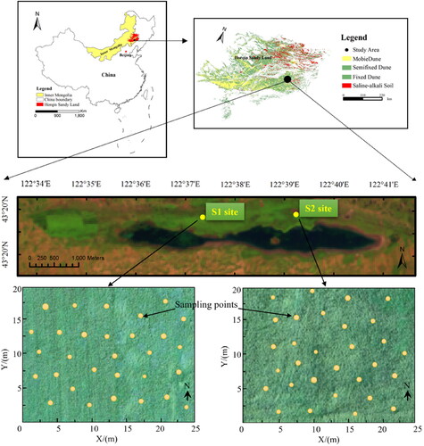
In situ experiments were set up in the study area (latitude 43°18′48′′N to 43°21′24′′N, longitude 122°33′00′′E to 122°41′00′′E) of Agula Eco-hydrological Experimental Station. It is located in the southern Horqin sandy land, eastern Inner Mongolia, Tongliao City, China. The climate is monsoon-influenced temperate semiarid with hot moist summers and cold windy dry winters, a long-term mean annual rainfall of 389 mm and a mean annual temperature of 6.6 °C (Tong et al. 2016).

Sand-grassland ecotone is the main geomorphologic characteristic of the study area, and there is a long narrow lake in the middle part. The grasslands are the major economic basis for the people living there, providing forage for livestock, e.g. cattle, sheep, horses and goats. Livestock grazing and forage planting are two dominant types of land use of the grasslands. The grazing strategies between three grazing systems in this area, controlled, rotational, and uncontrolled, vary considerably. Pasturing is forbidden during the whole growing season in the grasslands located around the lake, whereas forage harvesting usually begins in mid-July. The grass then dries, to be served as hay forage. Under the domestic grazing prohibition policy, livestock can be herded to the grasslands in the ecotones from July to the end of March of the next year. A small portion of grasslands, used as a rangeland specific to horses, is unrestricted.

Two sites within the grazing-controlled flat grasslands, S1 and S2, were chosen for experimental data collection (Figure 1). Leymus chinensis was the dominant plant species at S1 site. Besides the Leymus chinensis, S1 site also had a small proportion of Phragmites australis. But for S2 site, the dominating species, Phragmites communis, covers almost all of the area. The two sites were located in the grasslands with little topographic variability, which had no grazing histories for nearly a decade, and they offered the main forage supplies for a village located in the north.

Figure 1. Two experimental sites and sampling points in the study area.

2.2. Data collection

The FieldSpec HandHeld spectroradiometer (Analytical Spectral Devices, Inc., Boulder, CO, USA) was used for measuring the reflectance spectral data on August 13, 2015. It was a sunny, cloudless and windless day. This spectroradiometer measured the reflectance data in the wavelength domain from 325 nm to 1075 nm with a sampling interval of 1.5 nm and a resolution of 3.5 nm, and these measurements were resampled to spectra with 1 nm resolution by the manufacturer’s software. A post level was anchored to it to ensure nadir view (Figure 2a), resulting in a field of view (FOV) of 25° full conical angle. Before spectra measurements, the spectroradiometer was fully warmed up, and it was optimized and calibrated with a white reference Spectralon® panel (Labsphere, Inc., North Sutton, USA) with 100% reflectance, i.e. the spectrum reflected from the panel was used to normalize the spectrum reflected from each sample, for every 10 min or in case of solar illumination change.

Figure 2. (a) Post level anchored to the spectroradiometer. Schematic diagram of (b) sampling spectral reflectance, (c) cutting grass within the circumscribed quadrilateral of ground-projected FOV, and (d) square field calibration plot and circular ground-projected FOV of each sampling point.

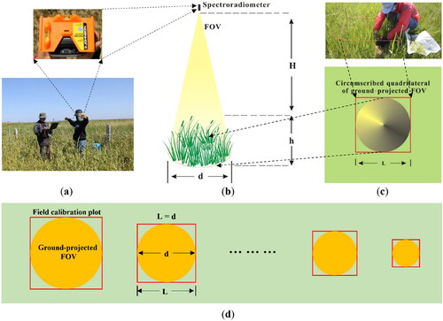
The reflectance measurements started at 12:10 and 13:05 local time (GMT + 8) and both lasted around 40 min on S1 and S2 sites, respectively. For each site we chose sampling points across a wide range of grass abundance from sparse to dense, and 30 points covering different grassland biomass levels were chosen. After measuring the canopy height at each point, the reflectance was sampled at a distance of 0.7 m at nadir above the grass canopy (Figure 2b). Spectra from three measurements were averaged, resulting in one spectrum per field point, which was used for further analysis. AGB sampling campaigns were carried out right after reflectance measurements. Considering the practical operability and feasibility and the need to minimize the mismatch in spatial scales between field calibration plots and ground-projected FOVs, for each sampling point the grass within a square area, which was the circumscribed quadrilateral of the ground-projected FOV, was cut at the ground surface (Figure 2c). In this way, although the field calibration plots were slightly larger than ground-projected FOVs (Figure 2d), the co-registration error that occurs between AGB and spectroradiometer samples was quite small due to the very high degree of spatial overlap between them (Frazer et al. 2011; Réjou-Méchain et al. 2014). The square areas at S1 site ranged from 0.57 to 1.65 m², and from 0.57 to 1.46 m² at S2 site. The grass was weighed immediately in the field to calculate the aboveground fresh biomass (AGFB, g m⁻²). Then, those grass samples were put into the ventilated oven at 105 °C for 30 min and then dried at 70 °C until the constant weight for the calculation of aboveground dry biomass (AGDB, g m⁻²).

2.3. Data analysis

In order to focus on the wavelengths most sensitive to vegetation characteristics, and to avoid the low signal-to-noise ratio of both sides of the reflectance spectrum, the spectral wavelength domain used in this study was 400-900 nm. The raw reflectance spectra were preprocessed with the mean filter smoothing to compute the first derivative spectra. A filter size of 5 nm was chosen, as smooth derivative spectra could be obtained and a coarse resolution may result in the loss of spectral details. The first derivative reflectance was defined as (1) $$\mathrm{FDR}\left({\lambda }_i\right)=\frac{R\left({\lambda }_i\right)-R\left({\lambda }_j\right)}{\mathrm{\Delta }\lambda }$$(1) where $\mathrm{ }\mathrm{FDR}({\lambda }_i)$ is the first derivative reflectance at wavelength λ_i; R(λ_i) and R(λ_j) are the reflectances at wavelength λ_i and λ_j, respectively; and Δλ is the wavelength increment, Δλ = λ_i - λ_j and λ_i > λ_j. A large increment can cause the loss of important spectral features, however, artifacts can be introduced if a wavelength increment is smaller than the spectroradiometer spectral resolution. In this study, an increment of 5 was selected, which was equal to the mean filter size and slightly larger than the spectral resolution of the raw hyperspectral reflectance data.

The correlation analysis was done between the first derivative and raw reflectance at each of 501 individual narrow bands and the AGB at both sites. To overcome the limitations of fixed band VIs, all possible band combinations were subsequently used to construct the FDR-VIs and RR-VIs in the forms of four commonly used VIs, i.e. SR, NDVI, SAVI, and EVI (Table 1). The coefficient of determination (R²) of each band combination was determined using the linear regression analysis between FDR-VIs, RR-VIs and AGB, respectively. Then, optimal FDR-VIs (FDR-SR, FDR-NDVI, FDR-SAVI, and FDR-EVI) and RR-VIs (RR-SR, RR-NDVI, RR-SAVI, and RR-EVI), based on the waveband selection from all available wavelengths, were determined.

Table 1. Selected VIs used in this study.

Index	Designation	Equation	References
SR	Simple ratio vegetation index	$\mathrm{SR}=\frac{{\rho }_1}{{\rho }_2}$	Jordan (1969)
NDVI	Normalized difference vegetation index	$\mathrm{NDVI}=\frac{{\rho }_1-{\rho }_2}{{\rho }_1+{\rho }_2}$	Rouse et al. (1974)
SAVI	Soil adjusted vegetation index	$\mathrm{SAVI}=\frac{1.5({\rho }_1-{\rho }_2)}{{\rho }_1+{\rho }_2+0.5}$	Huete (1988)
EVI	Enhanced vegetation index	$\mathrm{EVI}=2.5\frac{({\rho }_1-{\rho }_2)}{{\rho }_1+{6\rho }_2-{7.5\rho }_3+1}$	Huete et al. (1997)

ρ_i refers to reflectance in band i.

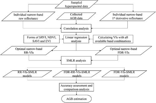
The SMLR models using four optimal FDR-VIs (FDR-VIs-SMLR models), four optimal RR-VIs (RR-VIs-SMLR models), and both FDR-VIs and RR-VIs (FDR-RR-VIs-SMLR models) as input variables were developed for estimating AGFB and AGDB. On the basis of the SMLR algorithm, the most predictive VIs from all available VIs were selected to build the predictive models with reduced variables. The flowchart of data processing and statistical analysis is shown in Figure 3.

Figure 3. Flowchart of data processing and statistical analysis in this study.

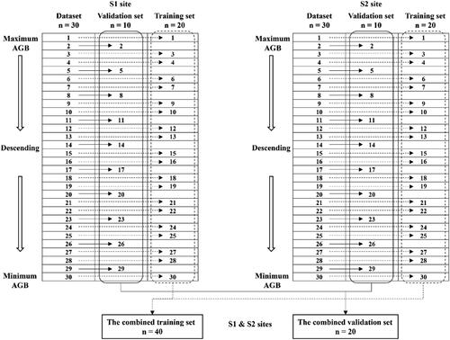
A ‘data-splitting’ approach similar to systematic sampling design was adopted to support regression model training and validation, with two-thirds of the entire dataset reserved for training and the rest one-third for validation (Figure 4). More specifically, as for S1 site and S2 site, 30 samples were ranked in descending order based on AGB values. Then starting from the second sample, every third sample was selected into validation dataset, and the remaining samples were put into training dataset, resulting in 20 samples reserved for training and 10 samples for validation at each site. Considering the limited amount of data, the leave-one-out cross-validation procedure was applied to optimize SMLR models. In cross-validation, each sample of training set was excluded in turn and the model was built with all remaining samples and used to predict that sample. Model performances were evaluated using the cross-validated coefficient of determination (R²_CV) and root-mean-square error (RMSE_CV). The optimized FDR-VIs-SMLR models, RR-VIs-SMLR models and FDR-RR-VIs-SMLR models with optimal VIs were subsequently developed using all samples in training dataset, and the samples in validation dataset were used for model validation with the R² and RMSE as evaluation metrics. In order to build a general AGB estimation model with chosen recommended VI variables, the training and validation datasets of both S1 and S2 sites were combined together as larger training (n = 40) and validation (n = 20) datasets for testing the applicability of the estimation model.

Figure 4. Strategy of dataset segmentation.

Data handling and analyses of linear regression and SMLR were implemented using MATLAB R2016a software (MathWorks, Inc., Natick, USA).

3. Results

3.1. Spatial variations of AGB

The descriptive statistics of AGFB and AGDB at both S1 and S2 sites show a wider interval of variability, i.e. an average of 3-fold variation (the ratio of maximum to minimum) in these two indicators (Table 2). For each site, even though sampling points were all in the same biome, the spatial discrepancy of AGB was still noticeable. The vegetation communities of the S1 and S2 sites are illustrated in Figure 5.

Figure 5. Vegetation communities of the S1 (a, b and c) and S2 (d, e, and f) sites.

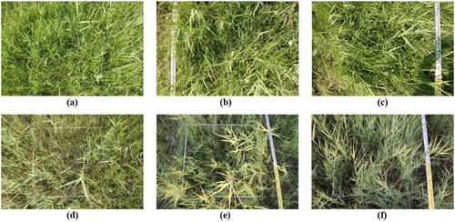
Table 2. Statistic parameters of the aboveground fresh biomass (AGFB) and dry biomass (AGDB) for the S1 and S2 sites, respectively (n = 30).

Indicator	Site	Minimum (g m^-2)	Maximum (g m^-2)	Range (g m^-2)	Mean (g m^-2)	Standard Deviation (g m^-2)
AGFB	S1	1009.99	3109.30	2099.31	1635.95	370.25
	S2	680.83	1695.60	1014.77	1338.43	232.72
AGDB	S1	287.94	919.06	631.12	490.30	107.09
	S2	245.39	712.59	467.20	534.67	111.61

3.2. Correlations between reflectance and AGB

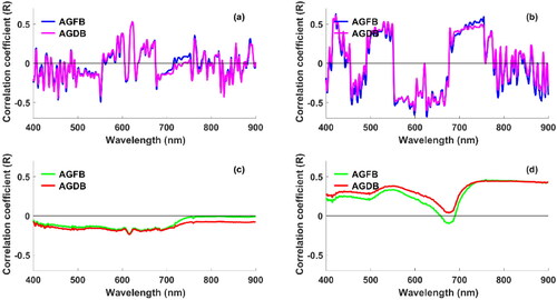
Correlograms were constructed by the sequential correlation analysis of the first derivative reflectance and raw reflectance at each of 501 individual narrow bands in the 400-900 nm domain against one type of AGB at a time and subsequent plotting of the correlation coefficient (R) against wavelength at both sites (Figure 6). For the S1 site, unlike the correlogram of raw reflectance and AGB, i.e. negative correlation was observed over the entire wavelength (Figure 6c), the correlogram of first derivative reflectance (FDR) and AGB fluctuated up and down around the “zero” line (Figure 6a), with no significant relationship regions. For the S2 site, six regions with relatively significant relationships between FDR and AGB were found: 415–429 nm, 450–475 nm, 502–550 nm, 554–602 nm, 625–669 nm and 689–755 nm (Figure 6b), whereas positive correlation was observed between two types of AGB and raw reflectance (RR) over the entire wavelength except for 650-700 nm spectral region in the correlogram of RR and AGFB (Figure 6d). Overall, the discrepancies of relationship between two indicators and FDR at each wavelength were small. The correlogram patterns of the S1 and S2 sites were quite different.

Figure 6. Correlograms derived from a correlation analysis of the first derivative (upper two figures) and raw reflectance (lower two figures) against AGFB and AGDB at the S1 (left two figures) and S2 (right two figures) sites, respectively.

3.3. Relationship between VIs and AGB

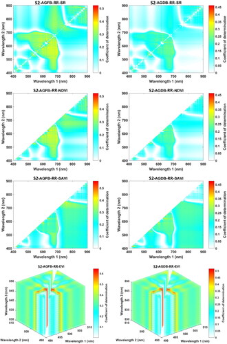
The matrix plots in Figures 7–10 illustrate the patterns of R² derived from the linear regression analysis between FDR-VIs and RR-VIs computed from all available narrow-band combinations and two indicators under study. Results of FDR-NDVI, RR-NDVI, FDR-SAVI, and RR-SAVI from the matrix below the diagonal were shown, since the R² values were symmetrically distributed along the diagonal in the plots. The matrix plots allowed the intuitive identification of waveband domains with high R² between the FDR-VIs and RR-VIs against the AGB. For each site, either for FDR-VIs or RR-VIs, similar R² patterns were observed for AGFB and AGDB due to the significant positive correlation between the two indicators. Irrespective of asymmetry, the patterns of FDR-SR and RR-SR were close to those of FDR-NDVI and RR-NDVI, respectively. It can be seen that the R² patterns of FDR-VIs and RR-VIs were quite different for each site, and the matrix plots of FDR-VIs against AGB showed a clear patchiness. In addition, for both FDR-VIs and RR-VIs, the R² patterns of the S1 site were different from that of the S2 site, and no broad expanse of the region with the highest R² values between 95% and 100% of the total best FDR-VIs or RR-VIs was noticeable for the two sites.

Figure 7. Matrix plots of the coefficient of determination (R²) between FDR-SR, FDR-NDVI, FDR-SAVI and FDR-EVI against AGFB and AGDB at the S1 site.

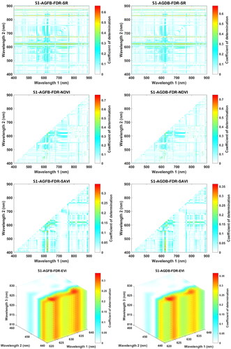
Figure 8. Matrix plots of the coefficient of determination (R²) between RR-SR, RR-NDVI, RR-SAVI and RR-EVI against AGFB and AGDB at the S1 site.

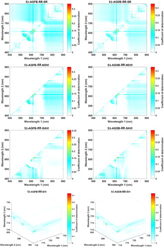
Figure 9. Matrix plots of the coefficient of determination (R²) between FDR-SR, FDR-NDVI, FDR-SAVI and FDR-EVI against AGFB and AGDB at the S2 site.

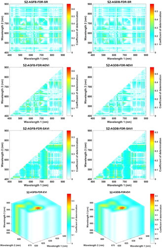
Figure 10. Matrix plots of the coefficient of determination (R²) between RR-SR, RR-NDVI, RR-SAVI and RR-EVI against AGFB and AGDB at the S2 site.

The optimal FDR-VIs and RR-VIs, based on all possible wavebands for simulating the two indicators at both sites, are given in Tables 3 and 4, respectively. For both S1 and S2 sites, the best fitting performances of the optimal RR-VI based on all available wavebands for AGB were provided by RR-EVI, with R² values of 0.730 and 0.688 for AGFB and AGDB at the S1 site, and R² values of 0.644 and 0.524 for AGFB and AGDB at S2 site. The best fitting performances of the optimal FDR-VIs were FDR-SR and FDR-NDVI at the S1 site, while four optimal FDR-VIs showed similar performance at the S2 site. Additionally, the selected spectral band combinations from entire available wavelengths for the RR-VIs were different with those for FDR-VIs.

Table 3. Optimal RR-VIs (darker background) and FDR-VIs against AGFB and AGDB based on all possible wavebands at the S1 site.

Index	Indicator	R^2	Band1	Band2	Band3	R^2	Band1	Band2	Band3
			(nm)	(nm)	(nm)		(nm)	(nm)	(nm)
SR	AGFB	0.335	623	622		0.660	816	872
	AGDB	0.327	494	491		0.677	816	872
NDVI	AGFB	0.333	623	622		0.758	804	650
	AGDB	0.326	494	491		0.748	804	650
SAVI	AGFB	0.353	624	622		0.346	887	829
	AGDB	0.332	624	622		0.363	623	445
EVI	AGFB	0.730	711	582	718	0.347	887	829	900
	AGDB	0.688	532	750	887	0.364	623	445	813

Spectral bands with purple, blue, green, yellow, red, magenta and black highlighting represent the violet, blue, green, yellow, red, red-edge and near-infrared wavebands, respectively. Waveband domains are defined according to Bruno and Svoronos (2006), and Sims and Gamon (2002).

Table 4. Optimal RR-VIs (darker background) and FDR-VIs against AGFB and AGDB based on all possible wavebands at the S2 site.

Index	Indicator	R^2	Band1	Band2	Band3	R^2	Band1	Band2	Band3
			(nm)	(nm)	(nm)		(nm)	(nm)	(nm)
SR	AGFB	0.523	594	592		0.670	683	538
	AGDB	0.462	827	820		0.587	498	539
NDVI	AGFB	0.523	594	592		0.649	683	538
	AGDB	0.461	827	820		0.578	498	539
SAVI	AGFB	0.560	627	624		0.578	626	679
	AGDB	0.474	496	490		0.518	626	679
EVI	AGFB	0.644	498	497	833	0.582	626	679	897
	AGDB	0.524	488	490	900	0.521	626	679	897

Spectral bands with blue, green, orange, red and black highlighting represent the blue, green, orange, red and near-infrared wavebands, respectively. Waveband domains are defined according to Bruno and Svoronos (2006), and Sims and Gamon (2002).

3.4. SMLR models optimized for AGB

Table 5 presents the results of the SMLR models using the most sensitive RR-VIs (RR-VIs-SMLR models), the most sensitive FDR-VIs (FDR-VIs-SMLR models), and the combined most sensitive FDR-VIs and RR-VIs (FDR-RR-VIs-SMLR models) for estimating AGFB and AGDB at both sites. The estimation performances of FDR-VIs-SMLR models were slightly better than that of RR-VIs-SMLR models for both training and validation datasets at the S1 site. As for the S2 site, the FDR-VIs-SMLR models showed similar performance to the RR-VIs-SMLR models with an increase in RMSE_CV of 4.29% for AGFB and a decrease in RMSE_CV of 8.82% for AGDB for the training sets, and a decrease in RMSE of 2.79% for AGFB and an increase in RMSE of 24.19% for AGDB for the validation sets. Compared with the previous two types of models, the FDR-RR-VIs-SMLR models had better performance with higher R²_CV (maximum increase of 17%) and lower RMSE_CV (maximum decrease of 30%) for the training datasets, and higher R² (maximum increase of 61%) and lower RMSE (maximum decrease of 44%) for the validation datasets.

Table 5. Results of the SMLR models using best RR-VIs, FDR-VIs, and fused RR- and FDR-VIs with related accuracy parameters for estimating AGFB and AGDB of two sites.

Site	Indicator	FDR-RR-VIs-SMLR model					FDR-VIs-SMLR model					RR-VIs-SMLR model
		Index	Training (n = 20)		Validation (n = 10)		Index	Training (n = 20)		Validation (n = 10)		Index	Training (n = 20)		Validation (n = 10)
			R^2CV	RMSECV	R^2	RMSE		R^2CV	RMSECV	R^2	RMSE		R^2CV	RMSECV	R^2	RMSE
				(g m^-2)		(g m^-2)			(g m^-2)		(g m^-2)			(g m^-2)		(g m^-2)
S1	AGFB	EVI SAVI’	0.76	172.94	0.74	167.72	NDVI’ SAVI' EVI’	0.81	173.39	0.70	174.05	SR EVI	0.78	179.91	0.65	180.37
	AGDB	SR NDVI SR' NDVI’ EVI’	0.85	45.19	0.71	47.70	NDVI’ EVI’	0.80	52.29	0.64	48.73	EVI	0.73	61.79	0.48	52.43
S2	AGFB	SR NDVI SAVI SAVI’ EVI’	0.90	78.03	0.68	167.91	NDVI’ SAVI' EVI’	0.79	111.78	0.50	171.00	SR NDVI SAVI	0.80	107.18	0.57	175.91
	AGDB	SR NDVI SAVI EVI SAVI’ EVI’	0.80	50.67	0.81	44.74	SR’ NDVI’ SAVI’ EVI’	0.77	54.63	0.51	80.28	SR SAVI EVI	0.72	60.33	0.66	64.64

VI’ refer to the FDR-VI.

The general recommended model employing the same preferred VI variables, using separate training and validation datasets, as well as the combined training and validation datasets for estimating AGFB and AGDB was determined (Table 6). The RR-SAVI, RR-EVI, FDR-NDVI, FDR-SAVI, and FDR-EVI were the five most preferred input VI variables to develop the recommended FDR-RR-VIs-SMLR model, which overall provided better estimating performance for AGFB than for AGDB. The AGFB validation results from the general recommended FDR-RR-VIs-SMLR model were shown in Figure 11.

Figure 11. Scattergrams of measured versus estimated AGFB using the recommended FDR-RR-VIs-SMLR model with the combined validation dataset (a), separate validation datasets of S1 site (b) and S2 site (c).

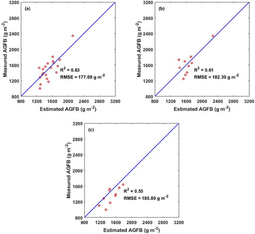
Table 6. Accuracy parameters of the recommended FDR-RR-VIs-SMLR model using the preferred VI variables for estimating AGFB and AGDB.

Index	Indicator	S1 & S2 sites (n = 60)				S1 site (n = 30)				S2 site (n = 30)
		Training (n = 40)		Validation (n = 20)		Training (n = 20)		Validation (n = 10)		Training (n = 20)		Validation (n = 10)
		R^2CV	RMSECV	R^2	RMSE	R^2CV	RMSECV	R^2	RMSE	R^2CV	RMSECV	R^2	RMSE
			(g m^-2)		(g m^-2)		(g m^-2)		(g m^-2)		(g m^-2)		(g m^-2)
SAVI EVI NDVI' SAVI' EVI'	AGFB	0.76	176.39	0.63	177.09	0.77	174.77	0.61	182.30	0.84	58.82	0.55	185.89
	AGDB	0.45	87.82	0.40	71.91	0.75	46.27	0.50	51.05	0.73	47.51	0.69	56.16

VI’ refer to the FDR-VI.

4. Discussion

4.1. Local spatial variations of AGB

Grassland areas often show considerable soil, topography and species heterogeneity (Bretas et al. 2021). At a small spatial scale, local spatial variability of AGB represented in this study was noticeable (Table 2). This is because environmental factors, such as micro-topography, soil property, water and heat status of a relatively small region, still have spatial heterogeneity, which consequently impacts spatial variations of AGB in grasslands at small scales (Gasch et al. 2015; Tamme et al. 2016).

4.2. Correlations between reflectance and AGB

Differences in vegetation communities and their canopies at the two sites resulted in different correlogram patterns of either RR or FDR and AGB (Figure 6). As shown in Figure 5, the vegetation canopy at S1 site was denser than that at S2 site, consequently, the impact of saturation problem was more pronounced for S1 site, as the correlograms were less undulating and correlation between raw red and NIR reflectance and AGB was weaker. The grass density, cover, geometric characteristics of canopy (e.g. leaf size, shape, angle and stratification), species composition, and richness of the two sites were factors influencing the biophysical relationship between the raw spectral reflectance and AGB (Campos et al. 2014; Zhang et al. 2021), hence the correlation relationships between the raw individual waveband reflectance and AGB were weak (Figure 6c and d). However, the correlations between the most sensitive FDR and AGB were much better than those between the most sensitive RR and AGB. These results confirmed that the derivative of the raw reflectance (i.e. FDR spectra) is a useful way to reduce the effect of low-frequency noise (soil background) and enhance subtle and weak canopy spectral features, thereby producing more straightforward and better correlations (Demetriades-Shah et al. 1990; Chen et al. 2010; Gnyp et al. 2014b; Liang et al. 2018). In addition, six relatively significant correlation regions between FDR and AGB for S2 site involve all visible wavelengths, except for the near-infrared wavelengths, indicating that for less dense vegetation canopies the sensitive fluctuation of the correlation between FDR in the multiple scattering NIR bands and AGB was greater than that in the visible absorption bands.

4.3. Optimal VIs based on all possible wavebands against AGB

Among all the optimal RR-VIs and FDR-VIs, only the wavebands of optimal FDR-NDVIs against AGFB and AGDB at S1 site belonged to the traditionally used wavelengths, i.e. near-infrared and red bands for NDVI. Other optimal VIs were all computed with band combinations from all available wavebands instead of traditional waveband extents. This emphasized the importance of taking advantage of full-extent suitable narrow wavebands to construct the optimal VIs for AGB estimation. These selected important wavebands were mainly distributed at red (including red-edge) bands, such as 622 nm to 627 nm, 650 nm, 679 nm, 683 nm, 711 nm, 718 nm and 750 nm, and near-infrared bands, such as 804 nm to 833 nm, 872 nm, 887 nm to 900 nm. The red and near-infrared bands occupied 37.50% and 29.17% of all selected wavebands, respectively. The red and near-infrared waveband regions were the most useful for computation of optimal VIs to simulate the grassland AGB (Jiang et al. 2008; Bayaraa et al. 2021).

4.4. Evaluation of SMLR models optimized for AGB

The most sensitive narrow two- or three-band combination RR-VIs used in RR-VIs-SMLR models extended spectral features from the one-dimensional scale to two- or three-dimensional scale. Thus, they can provide additional spectral information beyond the weak correlation between the individual RR and AGB, and effectively improve the sensitivity to AGB. Bayaraa et al. (2021) developed linear regression models with different VIs to estimate AGDB in Mongolian grassland, and their best results for all data were R² value of 0.62 and RMSE value of 60.96 g m⁻². For both training and validation datasets at both S1 and S2 sites, the optimal RR-VIs-SMLR models in this study showed better performance (Table 5). Nevertheless, the ultimate estimating performance might be influenced by the fact that narrow band RR-VIs extracted not only the significant spectral signals but also low-frequency noise (Aneece et al. 2017; Liang et al. 2018). Overall, the estimation performances of the FDR-VIs-SMLR models were comparable with that of RR-VIs-SMLR models. Gnyp et al. (2014b) developed the optimum multiple narrow band reflectance models using the SMLR method for estimating the rice AGB at later growth stage with high canopy closure. They also found that the FDR-based and the RR-based regressions produced nearly the same degree of performance. Under the derivative transformation, the optimal FDR-VIs calculated from all available narrow-band reflectance combinations could reduce the influence of low-frequency noise or trends, and enhance the weak spectral characteristics as compared with RR-VIs. However, the derivative processing may also cause the loss of some potentially useful spectral features related to the AGB, and the high-frequency noise would be amplified, and the signal-to-noise ratio would be reduced (Kharintsev and Salakhov 2004; Cheng et al. 2021). As a result, the estimation accuracy of FDR-VIs-SMLR models was still limited.

Compared to the FDR-VIs-SMLR and RR-VIs-SMLR models, the FDR-RR-VIs-SMLR models that integrated with the best FDR-VIs and RR-VIs performed better both for the training and validation datasets (Table 5). This methodology allowed increasing the accuracy of both indicators’ estimation at the two sites, with minimum relative mean absolute error of 4.7% and maximum relative mean absolute error of 11.0% for training datasets, as well as minimum relative mean absolute error of 6.8% and maximum relative mean absolute error of 12.1% for validation datasets. This indicates that the earlier mentioned two shortcomings of using only one type of VIs were overcome by the FDR-RR-VIs-SMLR model, which is a useful approach for more accurate prediction of the AGB at high productive growth stages. Consistent with the findings of Tao et al. (2020), the estimates of AGB obtained using a combination of optimal RR-VIs and FDR-based parameters were superior to those using optimal RR-VIs or FDR-based parameters standalone.

The normalized forms, soil adjusted forms and three-band EVI forms of narrow-band VIs played an important role in AGB estimation with the generally recommended FDR-RR-VIs-SMLR model at the peak productive growth stage when vegetation canopy almost totally covered the soil surface (Table 6), indicating that they have the capability to avoid the saturation of traditional broad-band VIs to a certain extent, although there was a slight underestimation in areas with high values of AGB, due to saturation effects (Figure 11). A similar result was found in a previous study, which found that narrow-band three-band VIs, such as EVI and visible atmospherically resistant index (VARI), were able to partly overcome the saturation problems (Zhang et al. 2021). In addition, AGFB might be a better indicator for herbage yield for grasslands because the process of acquiring AGFB is less complicated than that of AGDB, although AGFB and AGDB are both basic indicators of herbage yield of a grassland. Similar results could be found in the studies of Boschetti et al. (2007).

The significant optimal FDR-VIs and RR-VIs were chosen by the FDR-VIs-SMLR and RR-VIs-SMLR models which had a good accuracy in the AGB estimation at the two sites. In addition, the FDR-RR-VIs-SMLR models achieved further improvements. These results emphasized the benefit and potential of in-depth investigations of hyperspectral narrow band information (e.g. full spectral reflectance analysis, all available waveband extent VIs, derivative-based analysis, and combined use of multiple ways etc.) for developing more accurate AGB models (Tao et al. 2020). Even though hyperspectral remote sensing can provide high-dimensional sufficient spectral features, effective utilization of available spectral information from a large number of individual waveband reflectance is also a challenging task in the analysis of hyperspectral data. It has been shown that, compared to full width half maximum (FWHM), small shifts in band selection can lead to large differences in AGB estimates in grasslands (Fava et al. 2009). Selection of important hyperspectral remote sensed variables and modelling algorithms can significantly affect the performance of AGB estimation (Chen et al. 2009; Cheng et al. 2021). Indeed, VIs can suppress the influence of interference factors, such as canopy architecture, background effects, and the sensor and sun view-angles (Broge and Leblanc 2001; Boegh et al. 2002), and improve the vegetation spectral signature required for the accurate estimation of physiological and biochemical parameters of vegetation (Liang et al. 2015; Adams et al. 2021). Furthermore, derivative processing is a useful way to eliminate background signals, resolve overlapping spectral features, and enhance spectral contrast, thereby increasing the estimation accuracy of target information (Zhang et al. 2004; Wang et al. 2020). SMLR based on sensitive hyperspectral RR-VIs or FDR-VIs, especially on the application of both RR- and FDR-VIs, allowed to increase the accuracy of estimation of AGFB and AGDB, showing it as a reliable and appropriate method for accurate assessment of grassland productivity during the peak biomass period. Further research is needed to assess estimating the grassland AGB with optimal FDR- and RR-VIs using hyperspectral UAV or satellite images, together with other auxiliary information like texture metrics and topography data to further increase the estimation accuracy.

5. Conclusions

This study evaluated the ability to improve the estimation of grassland aboveground biomass (AGB) at the peak productive growth stage relative to the stepwise multiple linear regression (SMLR) models using optimal raw reflectance vegetation indices (RR-VIs-SMLR models) by the use of SMLR models using optimal first derivative reflectance vegetation indices (FDR-VIs-SMLR models) and both FDR-VIs and RR-VIs (FDR-RR-VIs-SMLR models). Field spectroradiometer and AGB data collected from grasslands under natural conditions without fertilization, constituted the primary data for this study. We conclude that with suitable band combinations, the SMLR models using optimized FDR-VIs or RR-VIs can produce good estimates of grassland AGB at the peak biomass stage. Via the derivative analysis, FDR-RR-VIs-SMLR models can further improve the accuracy of AGB estimation over FDR-VIs-SMLR and RR-VIs-SMLR models by incorporating both FDR-VIs and RR-VIs. This is an important step for more accurate forage yield estimation and harvest decision.

Disclosure statement

No potential conflict of interest was reported by the authors.

Data availability statement

The data supporting the findings of this study are available from the corresponding author upon reasonable request.

Additional information

Funding

This study was financially supported by the Inner Mongolia Agricultural University High-level Talents Research Launch Fund Project (NDYB2017-24), the National Natural Science Foundation of China (Grant Nos 51809141, 52169002, 51939006, U2243234, and 51620105003), the Major Science and Technology Projects of Inner Mongolia Autonomous Region (2020ZD0009), the Science and Technology Plan Project of Inner Mongolia Autonomous Region (2022YFSH0105 and 2021GG0071), the Inner Mongolia Natural Science Foundation (Grant Nos 2018BS05001 and 2018ZD05), the Ministry of Education Innovative Research Team (IRT_17R60), the Ministry of Science and Technology Innovative Team in Priority Areas (2015RA4013), the Inner Mongolia Autonomous Region Science and Technology Leading Talent Team (2022LJRC0007) and the Inner Mongolia Industrial Innovative Research Team (Grant No. 2012). The authors would like to thank the reviewers for their useful comments.

References

- Adams CB, Ritchie GL, Rajan N. 2021. Cotton phenotyping and physiology monitoring with a proximal remote sensing system. Crop Sci. 61(2):1317–1327.
- Aneece IP, Epstein H, Lerdau M. 2017. Correlating species and spectral diversities using hyperspectral remote sensing in early-successional fields. Ecol Evol. 7(10):3475–3488.
- Barrachina M, Cristóbal J, Tulla AF. 2015. Estimating above-ground biomass on mountain meadows and pastures through remote sensing. Int J Appl Earth Obs Geoinf. 38:184–192.
- Bayaraa B, Hirano A, Purevtseren M, Vandansambuu B, Damdin B, Natsagdorj E. 2022. Applicability of different vegetation indices for pasture biomass estimation in the north-central region of Mongolia. Geocarto Int. 37(25):7415–7430.
- Boegh E, Soegaard H, Broge N, Hasager CB, Jensen NO, Schelde K, Thomsen A. 2002. Airborne multispectral data for quantifying leaf area index, nitrogen concentration, and photosynthetic efficiency in agriculture. Remote Sens Environ. 81(2–3):179–193.
- Boschetti M, Bocchi S, Brivio PA. 2007. Assessment of pasture production in the Italian Alps using spectrometric and remote sensing information. Agric Ecosyst Environ. 118(1–4):267–272.
- Bretas IL, Valente DSM, Silva FF, Chizzotti ML, Paulino MF, D’Áurea AP, Paciullo DSC, Pedreira BC, Chizzotti FHM. 2021. Prediction of aboveground biomass and dry-matter content in Brachiaria pastures by combining meteorological data and satellite imagery. Grass Forage Sci. 76(3):340–352.
- Broge NH, Leblanc E. 2001. Comparing prediction power and stability of broadband and hyperspectral vegetation indices for estimation of green leaf area index and canopy chlorophyll density. Remote Sens Environ. 76(2):156–172.
- Bruno TJ, Svoronos PDN. 2006. CRC handbook of fundamental spectroscopic correlation charts. Boca Raton: CRC Taylor & Francis; p. 2006.
- Campos I, Neale CMU, López M-L, Balbontín C, Calera A. 2014. Analyzing the effect of shadow on the relationship between ground cover and vegetation indices by using spectral mixture and radiative transfer models. J Appl Remote Sens. 8(1):083562.
- Chen J, Gu S, Shen M, Tang Y, Matsushita B. 2009. Estimating aboveground biomass of grassland having a high canopy cover: an exploratory analysis of in situ hyperspectral data. Int J Remote Sens. 30(24):6497–6517.
- Chen P, Haboudane D, Tremblay N, Wang J, Vigneault P, Li B. 2010. New spectral indicator assessing the efficiency of crop nitrogen treatment in corn and wheat. Remote Sens Environ. 114(9):1987–1997.
- Cheng H, Wang J, Du Y, Zhai T, Fang Y, Li Z. 2021. Exploring the potential of canopy reflectance spectra for estimating organic carbon content of aboveground vegetation in coastal wetlands. Int J Remote Sens. 42(10):3850–3872.
- Costa V, Serôdio J, Lillebø AI, Sousa AI. 2021. Use of hyperspectral reflectance to non-destructively estimate seagrass Zostera noltei biomass. Ecol Indic. 121:107018.
- Curran PJ, Dungan JL, Gholz HL. 1990. Exploring the relationship between reflectance red edge and chlorophyll content in slash pine. Tree Physiol. 7(1_2_3_4):33–48.
- Demetriades-Shah TH, Steven MD, Clark JA. 1990. High resolution derivative spectra in remote sensing. Remote Sens Environ. 33(1):55–64.
- Eon RS, Goldsmith S, Bachmann CM, Tyler AC, Lapszynski CS, Badura GP, Osgood DT, Brett R. 2019. Retrieval of salt marsh above-ground biomass from high-spatial resolution hyperspectral imagery using PROSAIL. Remote Sens. 11(11):1385.
- Fava F, Colombo R, Bocchi S, Meroni M, Sitzia M, Fois N, Zucca C. 2009. Identification of hyperspectral vegetation indices for Mediterranean pasture characterization. Int J Appl Earth Obs Geoinf. 11(4):233–243.
- Fava F, Parolo G, Colombo R, Gusmeroli F, Della Marianna G, Monteiro AT, Bocchi S. 2010. Fine-scale assessment of hay meadow productivity and plant diversity in the European Alps using field spectrometric data. Agric Ecosyst Environ. 137(1–2):151–157.
- Foster AJ, Kakani VG, Mosali J. 2017. Estimation of bioenergy crop yield and N status by hyperspectral canopy reflectance and partial least square regression. Precision Agric. 18(2):192–209.
- Frazer GW, Magnussen S, Wulder MA, Niemann KO. 2011. Simulated impact of sample plot size and co-registration error on the accuracy and uncertainty of LiDAR-derived estimates of forest stand biomass. Remote Sens Environ. 115(2):636–649.
- Fricke T, Wachendorf M. 2013. Combining ultrasonic sward height and spectral signatures to assess the biomass of legume–grass swards. Comput and Electron Agric. 99:236–247.
- Gao X, Huete AR, Ni W, Miura T. 2000. Optical–biophysical relationships of vegetation spectra without background contamination. Remote Sens Environ. 74(3):609–620.
- Gasch CK, Huzurbazar SV, Stahl PD. 2015. Small-scale spatial heterogeneity of soil properties in undisturbed and reclaimed sagebrush steppe. Soil till Res. 153:42–47.
- Gnyp ML, Bareth G, Li F, Lenz-Wiedemann VIS, Koppe W, Miao Y, Hennig SD, Jia L, Laudien R, Chen X, et al. 2014a. Development and implementation of a multiscale biomass model using hyperspectral vegetation indices for winter wheat in the North China Plain. Int J Appl Earth Obs Geoinf. 33:232–242.
- Gnyp ML, Miao Y, Yuan F, Ustin SL, Yu K, Yao Y, Huang S, Bareth G. 2014b. Hyperspectral canopy sensing of paddy rice aboveground biomass at different growth stages. Field Crop Res. 155:42–55.
- He L, Li A, Yin G, Nan X, Bian J. 2019. Retrieval of grassland aboveground biomass through inversion of the PROSAIL model with MODIS imagery. Remote Sens. 11(13):1597.
- Huete AR, Liu HQ, Batchily K, van Leeuwen W. 1997. A comparison of vegetation indices over a global set of TM images for EOS-MODIS. Remote Sens Environ. 59(3):440–451.
- Huete AR. 1988. A soil-adjusted vegetation index (SAVI). Remote Sens Environ. 25(3):295–309.
- Jiang Z, Huete AR, Didan K, Miura T. 2008. Development of a two-band enhanced vegetation index without a blue band. Remote Sens Environ. 112(10):3833–3845.
- Jordan CF. 1969. Derivation of leaf-area index from quality of light on the forest floor. Ecology. 50(4):663–666.
- Kanke Y, Tubaña B, Dalen M, Harrell D. 2016. Evaluation of red and red-edge reflectance-based vegetation indices for rice biomass and grain yield prediction models in paddy fields. Precision Agric. 17(5):507–530.
- Kharintsev SS, Salakhov MK. 2004. A simple method to extract spectral parameters using fractional derivative spectrometry. Spectrochim Acta A. 60(8-9):2125–2133.
- Kumar L, Mutanga O. 2017. Remote sensing of above-ground biomass. Remote Sens. 9(9):935.
- Li Y, Liu Y, Wu S, Wang C, Xu A, Pan X. 2017. Hyper-spectral estimation of wheat biomass after alleviating of soil effects on spectra by non-negative matrix factorization. Eur J Agron. 84:58–66.
- Li Z, Han G, Zhao M, Wang J, Wang Z, Kemp DR, Michalk DL, Wilkes A, Behrendt K, Wang H, et al. 2015. Identifying management strategies to improve sustainability and household income for herders on the desert steppe in Inner Mongolia, China. Agr Syst. 132:62–72.
- Liang L, Di L, Huang T, Wang J, Lin L, Wang L, Yang M. 2018. Estimation of leaf nitrogen content in wheat using new hyperspectral indices and a random forest regression algorithm. Remote Sens. 10(12):1940.
- Liang L, Di L, Zhang L, Deng M, Qin Z, Zhao S, Lin H. 2015. Estimation of crop LAI using hyperspectral vegetation indices and a hybrid inversion method. Remote Sens Environ. 165:123–134.
- Luo S, Wang C, Xi X, Pan F, Peng D, Zou J, Nie S, Qin H. 2017a. Fusion of airborne LiDAR data and hyperspectral imagery for aboveground and belowground forest biomass estimation. Ecol Indic. 73:378–387.
- Luo S, Wang C, Xi X, Pan F, Qian M, Peng D, Nie S, Qin H, Lin Y. 2017b. Retrieving aboveground biomass of wetland Phragmites australis (common reed) using a combination of airborne discrete-return LiDAR and hyperspectral data. Int J Appl Earth Obs Geoinf. 58:107–117.
- Mahajan GR, Pandey RN, Sahoo RN, Gupta VK, Datta SC, Kumar D. 2017. Monitoring nitrogen, phosphorus and sulphur in hybrid rice (Oryza sativa L.) using hyperspectral remote sensing. Precision Agric. 18(5):736–761.
- Marshall M, Thenkabail P. 2015. Developing in situ non-destructive estimates of crop biomass to address issues of scale in remote sensing. Remote Sens. 7(1):808–835.
- Moeckel T, Safari H, Reddersen B, Fricke T, Wachendorf M. 2017. Fusion of ultrasonic and spectral sensor data for improving the estimation of biomass in grasslands with heterogeneous sward structure. Remote Sens. 9(1):98.
- Obermeier WA, Lehnert LW, Pohl MJ, Makowski Gianonni S, Silva B, Seibert R, Laser H, Moser G, Müller C, Luterbacher J, et al. 2019. Grassland ecosystem services in a changing environment: the potential of hyperspectral monitoring. Remote Sens Environ. 232:111273.
- Réjou-Méchain M, Muller-Landau HC, Detto M, Thomas SC, Toan TL, Saatchi SS, Barreto-Silva JS, Bourg NA, Bunyavejchewin S, Butt N, et al. 2014. Local spatial structure of forest biomass and its consequences for remote sensing of carbon stocks. Biogeosciences. 11(23):6827–6840.
- Rouse JW, Haas RH, Schell JA, Deering DW, Harlan JC. 1974. Monitoring the vernal advancement of retrogradation of natural vegetation. Greenbelt, MD: NASA/GSFC.
- Schucknecht A, Meroni M, Kayitakire F, Boureima A. 2017. Phenology-based biomass estimation to support rangeland management in semi-arid environments. Remote Sens. 9(5):463.
- Sims DA, Gamon JA. 2002. Relationships between leaf pigment content and spectral reflectance across a wide range of species, leaf structures and developmental stages. Remote Sens Environ. 81(2–3):337–354.
- Singh P, Srivastava PK, Mall RK, Bhattacharya BK, Prasad R. 2022. A hyperspectral R based leaf area index estimator: model development and implementation using AVIRIS-NG. Geocarto Int. 37(26):12792–12809.
- Tamme R, Gazol A, Price JN, Hiiesalu I, Pärtel M. 2016. Co-occurring grassland species vary in their responses to fine-scale soil heterogeneity. J Veg Sci. 27(5):1012–1022.
- Tao H, Feng H, Xu L, Miao M, Long H, Yue J, Li Z, Yang G, Yang X, Fan L. 2020. Estimation of crop growth parameters using UAV-based hyperspectral remote sensing data. Sensors. 20(5):1296.
- Tong X, Liu T, Singh VP, Duan L, Long D. 2016. Development of in situ experiments for evaluation of anisotropic reflectance effect on spectral mixture analysis for vegetation cover. IEEE Geosci Remote Sensing Lett. 13(5):636–640.
- Wang XY, Pan PP, Lu J. 2022. Estimation of shrubland aboveground biomass of the desert steppe from optical and C-band SAR data. Geocarto Int. 37(15):4509–4526.
- Wang Z, Zhang X, Zhang F, Chan N, Kung H-t, Liu S, Deng L. 2020. Estimation of soil salt content using machine learning techniques based on remote-sensing fractional derivatives, a case study in the Ebinur Lake Wetland National Nature Reserve, Northwest China. Ecol Indic. 119:106869.
- Wen P-F, He J, Ning F, Wang R, Zhang Y-H, Li J. 2019. Estimating leaf nitrogen concentration considering unsynchronized maize growth stages with canopy hyperspectral technique. Ecol Indic. 107:105590.
- Xu S, Zhao Y, Shi X, Wang M. 2017. Rapid determination of carbon, nitrogen, and phosphorus contents of field crops in China using visible and near-infrared reflectance spectroscopy. Crop Sci. 57(1):475–489.
- Zandler H, Brenning A, Samimi C. 2015. Potential of space-borne hyperspectral data for biomass quantification in an arid environment: advantages and limitations. Remote Sens. 7(4):4565–4580.
- Zhang J, Rivard B, Sanchez-Azofeifa A. 2004. Derivative spectral unmixing of hyperspectral data applied to mixtures of lichen and rock. IEEE Trans Geosci Remote Sens. 42(9):1934–1940.
- Zhang Y, Xia C, Zhang X, Cheng X, Feng G, Wang Y, Gao Q. 2021. Estimating the maize biomass by crop height and narrowband vegetation indices derived from UAV-based hyperspectral images. Ecol Indic. 129:107985.