Automated geometric precise correction of medium remote sensing images based on ASTER global digital elevation model

Abstract

Accurate and unified information from the increasingly remote sensing (RS) scenes is important for RS applications in multi-sectoral association services of natural resource management. However, these applications in mountain areas are limited by the challenging issues of random geometric distortions and erroneous spatial associations. The paper introduces digital elevation model (DEM) maps as a unified geographic reference to search and match homonymy ground points (HGPs). The proposed computer-based procedure was tested with Landsat TM, ETM and HJ-1B satellite images using ASTER global DEM in the Longitudinal Rang-gorge Valley Region of Southwest China. 1322, 3551 and 694 pairs of HGPs were identified and acquired the geometric accuracies with 43 m (TM), 14 m (ETM) and 123 m (HJ), respectively. The deviations are significantly reduced and the disjoint ground objects are matched. The study satisfies the application requirement of multispectral satellite imagery with less labour and time costs.

Keywords:

• Digital elevation model
• remote sensing image
• terrain feature lines
• ground control points
• geometric precise correction

1. Introduction

Remote sensing (RS) images are widely used in land-use/land-cover mapping, biodiversity protection, ecological disaster monitoring and other Earth surface dynamic monitoring. These applications usually rely on accurate and unified information from RS scenes (Kardoulas et al. 1996). However, there are contradictions between the increasingly developed RS data and application demands due to some limits of geometric precise correction, such as the random geometric distortions (Wu et al. 2019; Gu et al. 2010), the inconsistent projection coordinate systems (Wu et al. 2008), the geometric inconsistencies among multi-source base maps (Zheng et al. 2022), the difficulties of collecting adequate ground control points (GCPs) in mountainous areas (Han et al. 2019; Kardoulas et al. 1996), and the large labour and time costs of manual geometric precise correction (Ding et al. 2010). It is significant to overcome these limits and develop automatic techniques for geometric precise correction with high accuracy.

Geometric precise correction is one of the essential pre-processing operations in RS applications (Gu et al. 2010; Vogelmann et al. 2001; Jenson and Domingue 1988). Most RS optical images contain regional geometric distortions, which are introduced by the Earth curvature, topography, sensor and system and other interference sources. Even the RS images geo-referenced to L2 or L1T level still have random geometric distortions and erroneous spatial association (Devaraj and Shah 2014). The geometric accuracy of Landsat TM is found to be approximately on the order of 3–4 pixels, and HJ-1A/1B may reach 1 km. In most cases, adjacent RS scenes have some spatial dysconnectivity, characterized by deformations of lakes and breaks of rivers, roads, mountain valleys and other ground objects. Therefore, precisely eliminating these senseless errors is crucial for ensuring the accuracy of subsequent works, e.g. spatial overlying and joining analysis and mapping (Ye and Shan 2014).

Precise correction can be classified into two categories: image-to-image and image-to-map (Gianinetto and Scaioni 2008). For the case of image-to-image, a set of homologous ground control points are extracted from one reference image and are used by image-matching algorithms. However, no matter which algorithm is used, problems of geometric error transmits and accumulations exist eternally due to various shifts and rotations of the reference images. These issues would lead to a bad match with other geographic data in the follow-up work.

Another case of image-to-map uses a digital topographic map to derive ground control points to ensure that the derived information from RS images could be matched properly to other RS or geographic data. Previous studies have shown that large-scale topographic maps tend to be suitable for developed areas with dense road networks and river systems, and small-scale maps or GPS technologies obtain a resolution for developing areas where these recognizable features are not contained in a satellite image (Cheng and Po 2009; Smith and Atkinson 2001; Kardoulas et al. 1996). However, the projection coordinate systems of small-scale maps are often inconsistent in cooperation at the cross-regional level, and they are usually digitalized by the base topographic maps depicted by local surveying and mapping departments in varying periods. The digitalization process may produce equivocal geometric errors due to project transformation, map registration and manual vectorization. As well, both small-scale maps and GPS consume huge labour and time costs in mountainous areas where there is abundant natural resource information but complex terrains.

The above issues could be resolved by a reliable reference with enough ground control points in natural geographic areas. The ASTER global digital elevation model (DEM) with a resolution of 30 m and SRTM DEM with a resolution of 90 m are the two types of well-known global DEM data. They are available to all users with high geometric accuracy and frequently used coordinate systems (Rawat et al. 2019; Li et al. 2016). Technically, using DEM as the base topographic map can avoid the problems of inconsistency and low accuracy of previous references. One positive piece of evidence is that SRTM DEM has been employed to geo-reference the Landsat L1T images (Devaraj and Shah 2014). However, many crushed deformations still need to be corrected in mountainous areas. Meanwhile, rivers, roads and other traditional references for extracting ground control points are sparse and difficult to be identified out. Their spectral information is often submerged by other adjoining image objects in the low and moderate satellite images (Aguilar et al. 2013). These objects are not stable due to the intensifying human activities and seasonal volatility (Weser et al. 2008). DEM maps contain abundant terrain objects in mountainous areas, such as mountain ridges, valleys and other terrain features, which are widespread, readily available and relatively stable (Ding et al. 2010). Therefore, DEM maps are appropriate substitutes for the traditional references to collect GCPs.

To collect GCPs for batch processing, it is essential to design a computer-based procedure for searching and matching GCPs. Many reports focus on urban scenes and man-made or regular objects, e.g. buildings and individual trees (Fraser and Ravanbakhsh 2009; Inglada 2007; Chen et al. 2006). Few studies have investigated mountainous scenes and natural objects of mountain ridges and valleys, i.e. terrain feature lines (TFLs). For a Landsat TM scene, skilled professionals need to spend at least five to seven days manually searching over a thousand GCPs. Based on the experience, computer-based procedures provide assistance from two aspects: TFL extracting and GCP searching and matching from the TFL crossing or turning points. The matched GCP pairs refer to the same ground objects on the earth’s surface on both the DEM map and the RS images, so they are called homonymy ground points (HGPs) in this study.

Aiming at the random distortions of RS images in mountainous areas, this study presents an automated geometric precise correction method based on ASTER GDEM. First, by using a simple water flow simulation approach to extract TFLs from DEM maps, RS TFLs are obtained by introducing a marker-based watershed segmentation algorithm. Then, a computer-based procedure of HGP searching and matching from DEM maps and RS images is proposed. In this procedure, the arc-node topology of TFLs and their crossing points are identified for HGP searching, and three criteria are designed for HGP matching. The contributions of the proposed method to the desired efficiency are demonstrated by geometrically correcting Landsat TM, Landsat ETM and HJ-1B images in the mountains of the Longitudinal Rang-gorge Valley Region of Southwest China. The RS deviations with DEM terrain feature lines are significantly reduced, and the disjoint ground objects are matched.

2. Materials and methods

2.1. Study area

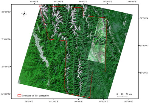
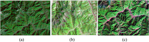
The experimental area is located in the Longitudinal Range-Gorge region of Yunnan Province, Southwest China. This mountain area has a complex topography and poor basic geographic information about rivers and roads. The three experimental RS images of Landsat TM, Landsat ETM and HJ-1B CCD were designed with different boundaries to verify the effects of correcting random geometric distortions in the junction of two image scenes and random geometric distortions over different images. Firstly, the TM image over the mountain area in Yunnan Province was clipped according to our archive DEM data, as shown by the boundary line in Figure 1. Secondly, the overlaying part of an HJ scene with the experimental TM scene was clipped out for the HJ correction experiment. Thirdly, the middle part of the HJ image was for the ETM. Visual interpretations show that the topographic deviation reaches several pixels among the RS images and between the RS image and the referencing DEM map. This indicates that the L2 or L1T RS products still contain significant geometric errors for the following qualitative or quantitative overlaying analysis.

Figure 1. The locations of the experimental Landsat TM, Landsat ETM and HJ-1B CCD images.

2.2. Data collection

The experimental RS images included a Landsat TM image, Landsat ETM image and HJ-1B CCD image, as shown in Figure 1. The Landsat TM image with a spatial resolution of 30 m, was captured on November 18, 2006. Its orbit path and row in its worldwide reference system are 130 and 043, respectively. Another experimental image is a part of the Landsat ETM scene with a spatial resolution of 15 m, captured on April 21, 2002. Its centre latitude and longitude are 24.55°and 109.27°, respectively. The third experimental image is the HJ-1B CCD image, which has a spatial resolution of 30 m and was captured on April 22, 2014. Its orbit path and row are 18 and 84, respectively. All the above images are Level 2 products, TM and HJ images were selected as representative RS data on a medium scale, and ETM was selected as higher-level data.

The experimental DEM data is ASTER DEM with a larger extent than the experimental RS images, and its resolution is 30 m. ASTER DEM is currently the most extensive coverage of global elevation data with high accuracy. It covers 99% of the land surface, and its resolution is the same as the main series of Landsat satellite images, which are the most widely used and effective RS data source for regional resources. By contrast, the publicly available SRTM global DEM only has a resolution of 90 m (Li et al. 2013). SRTM DEMs offer more precise elevation while ASTER DEMs offer more geomorphologic details (Bolch et al. 2005). Therefore, ASTER DEM is more suitable for the research goals than SRTM DEM.

2.3. Method

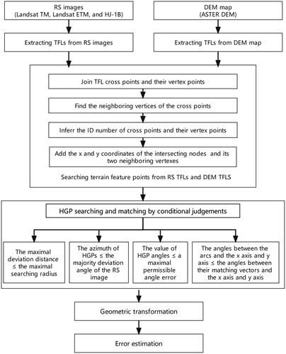
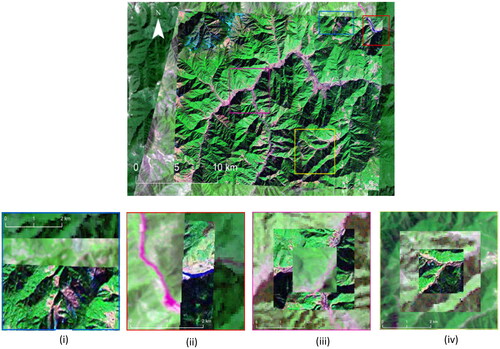
Geometric precise correcting RS images involves the following preliminary steps: extracting TFLs from DEM maps, extracting TFLs from RS images, searching terrain feature points from TFLs of RS images and DEM map, HGP searching and matching, geometric transformation, and error estimation. The flow of geometric correction is shown in Figure 2.

Figure 2. The flowchart of the geometric correction methodology.

2.3.1. Extracting TFLs from DEM maps

The water flow simulation approach has been proven to be effective for extracting TFLs from DEM maps. It describes the movement of surface flow from high to low elevations. Corresponding to hydrographic analysis, valleys of genuine topographic terrains are hydrographic basins and catchment areas of water. When the hydrographic flow accumulation of one cell in gully topography surpasses a predetermined threshold, the cell is considered a valley point. Therefore, valley lines of TFLs are the vectorized river networks in theory.

Based on this approach, identification of the cells for valley raster includes three steps: (1) calculate the flow direction grid from each cell to its steepest downslope neighbours (Jenson and Domingue 1988; Greenlee 1987); (2) produce the flow accumulation grid to by accumulating the for all that into downslope (Tarboton 1991; Jenson and Domingue 1988); (3) select pixels of valley lines by a speckle removal and thinning operation. In this process, an appropriate threshold value T needs to be defined by expertise or multiple experiments, which correlates to the DEM scale and cell size. Finally, valley line raster data are converted into vector data. Based on inversed computation of the DEM, high-elevation pixels are converted to low-elevation pixels, and the same approach is applied to extract points on ridge lines.

The study selects valley lines as the TFLs to identify the feature points because they are more straightforward to interpret than the ridge lines from anti-stereoscopic RS images and can supply a large number of control points. Based on the manual work of graduate students participating in the previous project and research, about two or three thousand feature points could be identified from the valley lines in a full Landsat TM scene (Ding et al. 2010).

2.3.2. Extracting TFLs from RS images

Matching with TFLs from DEM, automated extracting TFLs from RS images is equally important for searching control points. The pixel values of the digital RS image indicate the gray altitude of geo-objects. The highest or the lowest altitude pixels in a mountainous scene can be connected to feature lines of a mountain, i.e. TFLs. They are similar to ‘watershed lines’ of watershed segmentation, which is one of the image segmentation algorithms (Zhang and Wang 2009; Mei et al. 2004). Therefore, the study introduces the marker-based watershed segmentation algorithm to extract RS TFLs.

The marker-based watershed segmentation algorithm is a well-known image segmentation algorithm, which regards an image as a topography of geodesy and applies mathematical morphology to delineate the clustering objects by linear features (Mei et al. 2004). This study introduces this algorithm to extract TFLs from RS images. Two algorithm parameters needed to be predefined and provided to the running program: the radius of the circular structural element, and the square structural element. They work for labelling the foreground and background of the gray RS image to carry out morphological opening and closing, denoted by R and A.

However, the watershed segmentation process by mathematical matrix calculation will miss the coordinate information of the RS image. To address this issue, it is significant to add coordinate information to the segmented result to match with the original RS images. A worthwhile attempt is to export the RS image and the segmented image to BIL format and use the header file of the RS image to substitute that of the segmented image. The header file with a suffix‘.hdr’ contains the projection information that provides coordinates to display in GIS software. If this solution fails, image georeferencing will be a further solution.

2.3.3. Searching terrain feature points from TFLs of RS images and DEM map

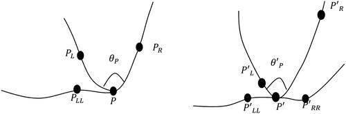
Cross points of TFLs are selected as terrain feature points owing to their identifiable information in computers. According to arc storage and indexing rules in ESRI ArcGIS software, one arc of TFL consists of a series of sequential indexed vertex points, of which the first vertex is called the from-node and the last vertex is the to-node. The node connecting two or more TFL arcs is a cross point, which is the from-node as well as to-node. As a vertex, a cross points possesses two or more vertex records and is numbered regularly in the vertex attribute tables. In addition, it has two or more neighbouring vertices, which are employed to match HGPs. Therefore, searching terrain feature points from TFLs of RS images and DEM maps is to identify the TFL cross points and their neighbouring vertices from RS images and DEM maps. There will be two resulting tables: one is for RS cross points and another is for DEM cross points.

Two attribute tables are related to our searching operation: the node attribute table and the vertex attribute table. The computer rules to identify the cross points and their neighbouring vertices can be defined by making use of their linked relationships and the internal ID numbers of these features. Depending on whether the vertex of the crossing point i.e. intersecting node, is the first vertex or the last in the connecting arc, the ID numbers of their neighbouring vertices are obtained (see Figure 3). The neighbouring vertex number is its vertex number plus one if it is the first vertex, or minus one if it is the last vertex. Denote a node with a vertex ID of FID, if the vertex is a ‘from-node’ in the arc (labeled FNOD in the node attribute table), its neighbouring vertex number is denoted as FID_Neighbor, then FID Neighbor = FID + 1; if a ‘to-node’ (labeled TNODE in the node attribute table), its neighbouring vertex number FID_Neighbor = FID + 1. The obtained ID numbers of the cross points and their neighbouring vertices can be used to relate with the node and the vertex table, thus associating with their XY coordinates for search and match HGPs.

Figure 3. The nodes and their neighbouring vertices in TFLs. The node P has three neighbouring vertices, of which the vertex P_L and P_R form the angle θ_P with P. P corresponds to the node P’ and the two nodes are a pair of HGP, where P’_L and P’_R form angle θ’_P with P’.

The procedure proposed for searching crossing points involves the following steps:

1. Build TFL topological relationships to obtain an indexed arc table.

2. Create node points for these arcs to obtain a node attribute table and add XY coordinates. If the node records in the node attribute table do not have internal numbers, an arc-node topology also needs to be built.

3. Extract all feature points from TFL arcs to produce a vertex attribute table and add XY coordinates.

4. Calculate the number of arcs connected to each node and select the nodes that connect more than two arcs.

5. Export the selected nodes to a new point file.

6. Join the selected node and vertex with the spatial join function by taking the selected nodes as target features and the vertex points as the join features. The joined result will identify the vertex ID numbers of the intersecting from-node and end-node from the vertex attribute table.

7. Find the neighbouring vertices of the selected nodes. Depending on the elaborated relationship between the vertex number of the crossing point and its neighbouring vertex number, the FID_Neighbor of each selected node can be inferred. By traversing all vertex records of the vertex attribute table, the neighbouring vertex numbers of the selected nodes are written to the above joined attributes table.

8. Add the x and y coordinates of the intersecting nodes $\left(P_x,P_y\right)$ and its two neighbouring vertexes $\left(P_{Lx},P_{Ly}\right)$ and $\left(P_{Rx},P_{Ry}\right).$ Relate the above output table with the node table and the vertex table by the selected node ID number and the vertex FID_Neighbor number, respectively. Finally, the XY coordinates of the intersecting nodes and their neighbouring vertices are prepared well to search and match HGPs.

2.3.4. HGP searching and matching

The cross points and their neighbouring points are associated with HGP searching and matching according to three criteria. From the manual experience of HGP collection, a pair of HGP in an L2 or L1T RS image and DEM map are the same ground objects with similar geometric shapes and the direction of geometric deviation, and their locations generally are in a range of several pixels. Accordingly, this study presents three criteria: the spatial neighbourhood selection criterion, the vector similarity criterion, and the similarity criterion of directional deviation. The spatial neighbourhood selection criterion indicates that the HGPs in an RS image are in a neighbourhood and a broad direction of its referencing HGP in the DEM. The vector similarity criterion indicates the TFLs connecting HGPs in RS images and DEMs must have similar geometry, including the angles and the vector line direction. The similarity criterion of directional deviation indicates that all HGPs in RS images offset in a general direction because the RS image usually exhibits an overall shift from its corresponding DEM.

HGP searching and matching is to find pairs of crossing points from RS images and the DEM map that satisfy the above criteria. With x and y coordinates of the crossing points and their neighbouring points, the three criteria for matching a point ($P$ in Figure 2) with its referencing point ($P^{\prime }$ in Figure 2) as a pair of HGP are represented as follows:

1. Supposing that $P$ is the point to be matched in the RS image, $P^{\prime }$ is the reference point in DEM, the Euclidean spatial distance ${L\_PP}^{\prime }$ between $P$ and $P^{\prime }$ satisfies ${L\_PP}^{\prime }\le D\_\max ,$ where $D\_\max$ is the maximal deviation distance determined by the accuracy of systematic correction, and it is a predefined parameter requiring interactions; ${L\_PP}^{\prime }$ is the maximal searching radius and can be calculated by the projected horizontal and vertical coordinates of $P$ and $P^{\prime }.$ Suppose the coordinates of the cross point $P$ and $P^{\prime }$ on a two-dimensional plane are respectively $\left(P_x,P_y\right)$ and $\left({P\prime }_x,{P\prime }_y\right),$ ${L\_PP}^{\prime }$ can be calculated as follows: (1) $${L\_PP}^{\prime }=\sqrt{{(P_x^{\prime }-P_x)}^2+{(P_y^{\prime }-P_y)}^2}$$(1)

2. $\lambda$ is the azimuth of $P^{\prime }$ relative to $P$ and $\phi$ is the majority angle of the RS image deviated from the geographic base map, then $\lambda \le \phi .$ The angle $\phi$ is the second parameter that needs to be predefined. Supposing the difference between $P_x$ and ${P\prime }_x$ is $\Delta \mathrm{x}$ and the difference between $P_y$ and ${P\prime }_y$ is $\Delta y,$ the azimuth $\lambda$ is calculated by the following sectional function:

3. By the vector similarity criterion, the value of HGP angles should be the same. ${\theta }_P$ and ${\theta }_{P\prime }$ satisfy $\left|{\theta }_P-{\theta }_{P\prime }\right|\le \delta .$ Here, $\delta$ is the HGP maximal permissible angle error, and it is the third interactive parameter. Supposing the projection coordinates of the left neighbouring point $P_L$ is $\left(P_{Lx},P_{Ly}\right),$ $\overrightarrow{a}$ is a vector formed by P and its neighbouring vertex $P_L,$ whose projected coordinates in the two-dimensional plane are $\mathrm{a}=\left\{\left(P_{Lx}-P_x\right),\left(P_{Ly}-P_y\right)\right\}.$ Similarly, P and $P_R$ constitute a vector $\overrightarrow{b}$ with the coordinates $\mathrm{b}=\left\{\left(P_{Rx}-P_x\right),\left(P_{Ry}-P_y\right)\right\},$ where $\mathrm{ }(P_{Rx},P_{Ry}$) is the projected coordinates of $P_R.$ Then, the angle ${\theta }_P$ is calculated by the following function: (2) $${\theta }_P=\mathit{arccos}\left[\frac{\left(P_{Lx}-P_x\right)\times \left(P_{Rx}-P_x\right)+\left(P_{Ly}-P_y\right)\times \left(P_{Ry}-P_y\right)}{\sqrt{{\left(P_{Lx}-P_x\right)}^2+{\left(P_{Ly}-P_y\right)}^2}\times \sqrt{{\left(P_{Rx}-P_x\right)}^2+{\left(P_{Ry}-P_y\right)}^2}}\right]\times \frac{180}{\pi }$$(2)

Similarly, the angle ${\theta }_{P\prime }$ between the reference feature point $P\prime$ and their neighbouring vertexes ${P\prime }_L$ and ${P\prime }_R$ can also be calculated.

1. Besides the value approximation, the crossing arcs should be in the same orientation. Denote ${\alpha }_L$ and ${\beta }_L$ as the angles between the vector $\overrightarrow{P{P}_L}$ and the $X$-axis and $Y$-axis, and denote ${ \alpha \prime }_L$ and ${\beta \prime }_L$ as the angles between their matching vector $\overrightarrow{P\prime {P\prime }_L}$ and the $X$-axis and $Y$-axis. Then, ${\alpha }_L-{\alpha \prime }_L\le \xi$ and ${\beta }_L-{\beta \prime }_L\le \xi ,$ where $\xi$ is the maximal angle offset that needs to be defined. Similarly, the other vector $\overrightarrow{ P{P}_R}$ and its corresponding vector $\overrightarrow{P\prime {P\prime }_R}$ also satisfy the above conditions. Take the calculation of ${\alpha }_L$ and ${\beta }_L$ as an example:

Depending on the above judgement rules, the computer procedure for searching and matching HGP is easy to be developed. Spatial searching steps by the first two rules will give a rough pair of control points in which the objective point in the RS image is related to several points in the DEM. Moreover, if the selected point pair satisfies ${\alpha }_L-{\alpha \prime }_L\le \xi ,$ ${\beta }_L-{\beta \prime }_L\le \xi ,$ and $\left|{\theta }_P-{\theta }_{P\prime }\right|\le \delta ,$ then the two points are considered as one HGP pair.

When multiple mountain ranges or gorges connect with the main big mountain or deep gorge, three or more angles will be formed by TFLs, just like that three angles will be formed by the neighbouring vertices $P_L,$ $P_R$ and $P_{LL}$ with the node P and four angles will be formed by the neighbouring vertices ${P\prime }_L,$ ${P\prime }_R,$ ${ P\prime }_{LL}\text{ and }{ P\prime }_{RR}$ with the node $P\prime$ in Figure 2. Each angle and direction of its side arcs need to be calculated and stored in the crossing point attribute tables for identifying the referencing angle for all the RS crossing points. It is suggested that the identification approach should calculate the directions of arc vectors first and search for the satisfying vectors. Then, the angle formed by the searched adjacent vectors is calculated to determine whether the current RS node is needed. Therefore, two loop programs should be designed in HGP searching and matching applications.

In the above, $D\_\max ,$ $\phi ,$ $\delta$ and $\xi$ are predefined parameters. They vary with the original parameters of RS images and the geometric accuracies of their previous corrections. Many trials are needed to obtain the desired results. Therefore, computer-based programs are recommended for these recycled processes. This study used ArcObjects in ArcGIS software to develop two interfaces for automated HGP searching and matching, where one interface is for identifying cross points with their coordinates and their adjacent vertex coordinates, and the other interface is for HGP searching and matching.

With the batch processing of the HGP searching and matching program, one-to-one control points cannot be matched very well due to an anomaly that two or more densely distributed reference points are related to one point. A delete operation might deal with this situation.

2.3.5. Geometric transformation

The Delaunay triangulation of the geometric transformation model and the nearest neighbour resampling method (Mei et al. 2002) are used to adjust the RS images. The triangle transformation divides the whole data surface into several triangles with the three nearest HGPs, and a local polynomial model is constructed for each triangle surface, where the correction is only related to the HGPs of the target triangle. Meanwhile, the nearest neighbour resampling method is employed to perform the fastest interpolation that assigns a pixel value by its nearest neighbour.

2.3.6. Error estimation

The point estimation method by sampling with a fishnet is adopted to estimate the geometric accuracy. First, a fishnet with a cell width of M and a height of M is created, and then n cells are selected randomly. Then, one or more pairs of control points are chosen from each selected cell, and the average distances from the corrected control points to their reference points are calculated. Next, error samples composed of the average distances $x_1,x_2,x_3,\dots \dots ,x_n$ of all selected cells are used to estimate the population error. If $n<30,$ the sample size meets the requirements of a small-sample hypothesis test. The geometric population error $\mathrm{\mu }$ of the corrected RS image is estimated by the mean error $\overline{x}$ as follows (Xu 2006): (3) $$\overline{x}=\frac{x_1+x_2+x_3,\dots \dots +x_n}{n}$$(3)

If the confidence level of $\mu$ is $1-\alpha ,$ the lower confidence limit is $\overline{x}-t_{\alpha /2}\times s/\sqrt{n}$ and the upper confidence limit is $\overline{x}+t_{\alpha /2}\times s/\sqrt{n},$ where $s$ is the sample standard error, and $s=\sqrt{\frac{{\sum }_{i=1}^n\left(x_i-\overline{x}\right)}{n-1}}.$

3. Results

3.1. TFLs and the feature points of DEM

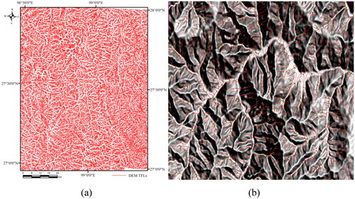
The threshold $T$ for selecting valley pixels was set to 10 in the water flow simulation procedure of extracting DEM TFLs. A large number of valley lines and their feature points were extracted from the DEM, as shown in Figure 4(a). 80,862 valley lines and 37,682 feature points were obtained over the experimental area of 19,662 km². Meanwhile, zoomed in to a mountain area of 472 km², 1984 valley lines and 884 feature points were obtained, as shown in Figure 4(b). This type of GCP significantly outnumbers traditional GCPs, like roads and rivers.

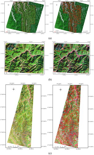
Figure 4. DEM TFLs of valleys in (a) part of the Longitudinal Range-Gorge region of Yunnan Province and their cross points in (b) the zoom-in area overlaid with the hill-shade texture.

By overlaying the extracted DEM valley lines, valleys generally had a deviation of several pixels in roughly the same direction. As shown in Figure 5(a,b), the TM image shifted northward, and the HJ image shifted southward overall. The geometric distortion of the ETM image was more complex as northward, southward and eastward shifts were distributed in different parts, as shown in Figure 5(c). By selecting several samples to measure these geometric errors, it was found that the maximum error of the TM image reached 300 m, and the minimum was greater than 100 m. Meanwhile, the geometric deviation of the HJ image was abnormally large, where the maximum error reached 1000 m. For the ETM image, the geometric deviation was about 100 m.

Figure 5. The deviation of DEM valley lines between (a) TM, (b) HJ and (c) ETM images.

As shown in Figure 6, there were many spatial discontinuities of the terrain features in the overlaid ETM, HJ and TM images, such as (i) the valleys in ETM and HJ images, (ii) the rivers in ETM and HJ images, (iii) the rivers in ETM, HJ and TM images and (iv) the valleys in ETM, HJ and TM images. This highlights the geometric inaccuracy in different images and will lead to the failure of integrated applications.

Figure 6. The spatially disjoint terrain features indicate geometric inaccuracies in the following integrated applications.

3.2. TFLs and feature points of RS images

The marker-based watershed segmentation generated a large number of TFLs and feature points from the experimental RS images, as shown in Figure 7. Through multiple attempts, the values of the two parameters R and A of the structural elements were determined to be 2 and 1 for the TM image, 20 and 2 for the HJ image and 22 and 5 for the ETM image, respectively. The experiments acquired 10,731 lines from the TM image over 19662 km² areas, 12,387 lines from the HJ image over 2386 km² areas and 14,263 lines from the ETM image over 472 km² areas. From these TM, HJ and ETM TFLs, the experiments automatically identified 7516, 7618 and 4982 crossing points, all of which were used as feature points for collecting HGPs. Visual interpretations show that the RS TFLs are primarily valley lines of large mountain bodies. It is consistent with the previous practices of visual interpretation and manual GCP selection that valley lines are more feasible to select GCPs. The distribution density of the RS TFLs is also significantly higher than that of the ordinary references.

Figure 7. The TFLs and HGPs of (a) the TM image, (b) the ETM image and (c) the HJ image.

The initial result of RS TFLs by vectoring operations contains lots of broken and short lines that lead to more feature lines than TFLs of DEM. By further removing the short lines, the number of RS TFLs dropped and was smaller than that of DEM TFLs, which determined the number of the final HGPs. Considering that the short lines are arcs with no cross points and would be filtered out in the next HGP matching operation, this study did not perform that delete operation.

3.3. HGP searching and matching

Through several experiments, the parameters of the three criteria for HGP searching and matching from RS images were set up, as shown in Table 1. Due to the biggest deviation, the value of D_max was set to 1 km, 500 m and 200 m for the HJ image, TM image and ETM image. Both the maximum angle and angle offset between two adjacent feature vectors were set to 15°, which represented that the permissible difference of angular maximum was 30°. The HGP searching azimuth range of the TM image and HJ image were defined as the first and the fourth quadrants according to the main shift azimuth. Omnidirectional searching was performed for the ETM image because of the random geometric shift in all directions.

Table 1. The parameters and the HGP pair numbers of the three types of experimented images.

RS image	D_max	$\delta$	$\zeta$	$\varphi$	HGP pairs
TM	500	15	15	$[0,90]\cup [270,360]$	1322
HJ	1000	15	15	$[0,90]\cup [270,360]$	3551
ETM	200	15	15	[0,360)	694

The number of HGP pairs was more than that of the traditional referencing elements. The procedure matched 1322, 3551 and 694 HGP pairs from TM, HJ and ETM feature points, respectively, as shown in Figure 7. If the traditional referencing elements, such as roads and rivers, were sampled as ground control points in these mountainous regions, only a few points could be obtained. After all, it is difficult to find multiple roads or rivers over high mountains from images with a resolution of 30 m or 25 m.

Our previous experiences with GCP manual collection indicate that manually about one thousand GCPs can be obtained manually from one scene of TM image in almost one week (Ding et al. 2010). Experimental results showed the orders of magnitude of HGP automated collection were as high as that of manual collection. It took twenty or thirty minutes for our computer with an Intel Core i3 3250M processor and 4GB main memory to perform automatic loops by a least efficient algorithm. This time-cost gap demonstrated that the time cost of the automated procedure was significantly lower than that of manual processing.

Experiment results showed the key factor affecting the numbers of matched HGPs was the parameter D_max instead of the corrected image area. Among the three RS images, the HJ image had a larger area but the most HGP pairs; on the contrary, the TM image had the largest area but more HGP pairs. This phenomenon was caused by the spatial neighbourhood selection procedure during the process of HGP searching and matching.

3.4. Visual interpretation of geometric correction results

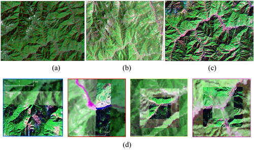
The visible comparison of the geometric correction results indicated that the deviation was significantly reduced and RS valleys were more consistent with DEM, as shown in Figure 8(a–c). Among the three experimented RS images, valleys in TM and ETM images highly matched with DEM valley lines, and therefore more impressive results were obtained. There were still some derivations in the HJ corrected image due to the large geometric offsets of the HJ original image. In addition, corrected by the unified references of DEM TFLs, the rivers, roads and mountain valleys in the three RS images were joined properly, as shown in Figure 8(d). The visual interpretation indicated that the correction procedure contributed to the desired effect.

Figure 8. The corrected (a) TM, (b) HJ and (c) ETM images overlaid with DEM TFLs and the disjoint ground objects were matched together of the three corrected images, as shown in (d) sub-maps.

3.5. Geometric accuracy

To obtain the geometric accuracy of the corrected images, a fishnet grid was first built and indexed. It was the same coverage as the TM image and its cells were set up to 500 m * 500 m size by the experienced knowledge. Then, 30 cells were randomly selected from the whole fishnet grid because 30 sampling points form a large sample population according to the mathematical sampling rule. And, a few cells with cloud covering were deleted. Next, a pair of HGP points was manually assigned to each sampling cell by overlaying the corrected image and the DEM map. The manually created points from the RS image were taken as the estimated ground points, and points from the DEM map were the true ground points. Finally, the distances of the HGP pair were measured to calculate the geometric accuracy.

Taking the TM image as an example, there were 27 cells with no cloud cover, and thus 27 error samples were obtained by measuring the Euclidean distance between each pair of sampling points, as shown in Table 2. By Formula (4), a mean error of these samples was generated at $\overline{x}$ = 43, and the standard error s = 19. If the confidence level was set to 90%, the experiment yielded $t_{0.1/2}(26)=1.71$ by looking up the bilateral quantile table of t-distribution with 27 degrees of freedom. The permissible error of the samples was 61, with an upper confidence limit of 49 and the lower confidence limit of 37. The above hypothesis test results indicated that the population error $\mu$ was 43 m, and the estimated interval of error was (37 m, 49 m). Also, the geometric mean error was less than 2 pixels of the RS image. Judging at a confidence level of 90%, the overall population error was on the order of 1.5 pixels. Considering that the permissible error for the GPC of RS images over mountainous areas is 2–3 pixels (Mei, et al. 2002), the experiment accuracy satisfies the requirements for most industries.

Table 2. The error samples of geometric precision correction.

ID	x (m)	ID	x (m)	ID	x (m)
1	33	10	21	19	43
2	58	11	78	20	13
3	18	12	28	21	61
4	42	13	54	22	42
5	39	14	34	23	29
6	47	15	47	24	42
7	41	16	37	25	72
8	72	17	43	26	16
9	84.	18	28	27	37

The geometric accuracies of most samples were less than 60 m, which is two pixels of the corrected TM image. The statistical overview of the error samples in Table 2 showed that the error of 7 samples was less than 30 m, the error of 15 samples was between 30 m and 60 m, and the error of 5 samples was between 60 m and 90 m. The larger errors happened in the cells with fewer control points. In the fishnet cells with low errors, there were more control points. This result is consistent with the characteristic of the Delaunay triangulation transformation.

The fishnets and sample cells for accuracy tests on ETM and HJ images were set up in the same way as the TM image, and 27 and 29 sample points respectively with no cloud covered were used. The mean geometric deviation in the corrected ETM image was 14 m, and the standard error was 14 m, whereas the mean error before the correction was 70 m. For the HJ image, the mean error was 741 m before correction and the corrected mean error was 123 m, with a standard error of 76 m. The corrections of ETM produced a mean absolute error at a pixel level, which was similar to the correcting result of the TM image. The mean error of the HJ image was at a level of four pixels, which was lower than that of TM and ETM images. This correction of HJ images still produced a significant effect compared with a mean error of 25 pixels before correction. The corrected RMSE errors for the three RS images were similar to the mean errors with small differences of about 0.5 pixels (Table 3).

Table 3. Error statistics for TM, HJ and ETM images before and after correction.

Errors	TM (m)		HJ (m)		ETM (m)
	Before	After	Before	After	Before	After
Mean	189	43	741	123	70	14
Std. dev.	47	18	185	76	41	14
Max	305	84	1039	379	158	43
Min	125	13	145	48	22	0
RMSE	192	46	750	142	80	19

4. Discussion

Fully utilizing RS image features and their physical representations helps to resolve the problems of traditional geometric precise correction in mountainous areas. A satellite image scene contains rich topographical information on mountainous areas, such as mountain ridges, valleys and other terrain features. Meanwhile, as one of the famous geographic base maps, the free DEM is relatively invariable. It can present most of these topographical features of mountains. Once these features are identified, the results could be saved in computers for correcting multi-images on a suitable scale. Therefore, DEM maps can be taken as a unified geographic reference that helps to avoid the problems of geometric error transmits and accumulations for the co-registration in an image-to-image manner. This uniform topographic reference is free, stable and well-known, and is thus more acceptable to users than an accidental referencing image or other topographic maps. The experiment results demonstrate that this solution can adjust random geometric distortions and erroneous spatial association in or among RS images, which facilities the geometric preprocessing for subsequent integration applications. Additionally, the HGPs obtained from valley lines and their crossing points indictate that the proposed methodology is only suitable in hilly areas and not suitable for plains or other areas where topographic features do not exist.

Both ASTER and SRTM DEMs contain sufficient topographical features of mountainous areas where the big mountains have many branches and bends that are large enough to show on these maps. Accuracy assessments in different regions showed that the errors of ASTER DEM range from −7.95 m to 26 m and that SRTM DEM range from −0.25 m to 23 m (Njimu and Odera 2019; Li et al. 2013; Zhao et al. 2011). The level of RMSE is equivalent to the pixel size of the Landsat TM images. The accuracy of ASTER DEM and SRTM DEM is negligible for the registration of these medium-resolution images because the control points are generally large mountain turns and crossings with several image pixels. In our previous study, 1175 HGPs were manually collected from SRTM over an area of over 1000 km² in the Anning region, Yunnan, China, and an average correction accuracy of no more than 1 pixel was obtained on the Landsat TM image (Ding et al. 2010). It seems that control points from RS images and HGP distribution have more impact on the correction accuracy. After all, as many as 500 feature points were extracted from an average area of 1 km² on a 30 m DEM by the experiment, and matching most of these points requires RS image enhancement or better feature extraction algorithms to increase the number of RS feature points.

The DEM scale and the threshold of flow accumulation determine the DEM TFL density (Li et al. 2014a; Sun et al. 2014; Valeo and Moin 2000). DEM with a resolution of 30 m can be used to adjust the medium-resolution images. When the scale is fixed, the higher the threshold, the sparser the TFLs. With a higher threshold, the feature lines of some important mountain bodies may be neglected, leading to the loss of many useful feature points. Conversely, when minor terrains are marked, excessive high-density TFLs will be created with too many short lines. The probable range of the thresholds can be determined by building a simple linear regression model based on the densities of hydrological networks (Li et al. 2014b). The study suggests that this threshold can be determined by multiple experiments and research experience.

Structural elements are critical to the marker-based watershed segmentation method. When the parameters of structural elements are set to large values, a significant number of control points and lines of major topography would be lost. Taking the TM image as an example, the sparse TFLs distributed across a few mountains when the parameters of the structural elements, i.e. R and A, were set to 5 and 6, respectively, while many mountain bodies were covered by dense TFLs when the parameters were set to 2 and 1, respectively. Some non-valleys and non-ridges with distinctive spectral features were identified as TFLs, such as the lines in the cloud-shaded regions. This is the limitation of the image segmentation algorithm, but it does not affect the study. Those non-TFLs only appear in some localities, and they do not have any correlation with the DEM feature lines. Those lines would be discarded in the subsequent matching operations.

Matching topographic feature points (or lines) is essentially matching the geometric points (or lines), and the general geometry matching methods are theoretically applicable. Previous studies proposed many measurement indicators for matching points or lines (Yasuda and Yin 2001). Some studies compared these indicators and found the matching based on the Euclidean geometric distance and direction achieved good results but had difficulty in selecting thresholds (Li et al. 2014c). The principles of matching HGPs in this paper are similar to the Euclidean distance measurement of point elements and the direction similarity measurement of linear elements. Therefore, there is also difficulty in confirming the thresholds of the measurement indicators, which demands pre-interpretation to identify the best values.

The TFLs present a significant influence on the control points. In mountainous areas with large relief, the valley lines can provide adequate control points for correction. Especially, in the case of a large number of cells with insufficient valley lines, inversing the DEMs to extract the feature points from ridge lines can complement the effective HGPs. Thus, after the geometric precision correction, the RS images can be better matched to the geographic base maps. In some flat lands with mild terrain undulation of a mountain area, the spectra of different slopes are similar, and the TFLs are undistinct because the RS images are subject to only minimal topographical influences. In this manner, fewer TFLs are provided. The solution to this problem is to design a fishnet and overlap it with the control point layer. Control points are manually added from rivers or roads. In addition, as a response to the characteristics of the self-adaptive TIN method, more control points with little deviation will be complemented for cells with insufficient control points.

The correction result is also affected by the original geometric accuracy of the input RS image. The L2 product of the HJ satellite image had a deviation of about 1 km (Xiong et al. 2014). The corrected result of the experimented HJ image exhibited a deviation of 200 m in some mountains. These regions need more corrections though the first correction had achieved considerable effects. More corrections need even fewer efforts such as manually adding a few control points.

Automation without user intervention is not feasible (Dare and Dowman 2001). Intervention is required to select optimal parameters for the feature extraction algorithms and verify the quality of the result. Experiments showed that manually capturing control points can reduce the geometric error to about one pixel (Ding et al. 2010). In most regions, the automated correction procedure can also match the pairs of GCPs to about one pixel. The registration accuracy is slightly lower in some special places. However, it is remarkably efficient in terms of time and labour consumption compared with the manual correction procedure.

5. Conclusions

Aiming to correct random geometric distortions and erroneous spatial association of RS images in mountainous areas, the study proposes an automated geometric precision correction based on DEM maps to overcome the limitations of the traditional topographic maps and the difficulties of GCP selection. The computer-based procedure for HGP searching and matching is illustrated by applying the arc-node topology and three criteria of cross points from DEM and RS TFLs. The experiments demonstrate that the number of automated HGPs is up to the order of magnitude of HGP manual collection, and the geometric accuracy satisfies the application requirement of meso-sale satellite imagery. The proposed method overcomes the difficulty of the traditional manual GCP selection and GPS measurement in vast mountainous areas. The study would fill in the gap of the increasing RS data and meet the demands for RS application, and it can be used in forestry, agriculture, land resource management, and monitoring with less labour and fewer time costs, especially in developing and underdeveloped countries where middle-resolution RS images are the dominating Earth observation data. The study shows that just using valley lines is likely to meet the demand for HGP collection. These HGPs can provide a sufficient sample space for building mathematical transformation models, constructing databases of known reference elements, and designing the spatial distribution of GCPs. By combing the methods of HGP searching and matching to construct an HGP database, the accuracy of other correction methods for satellite imagery could be further improved.

Moreover, the ASTER can provide sufficient HGPs in the skeletons of medium and big mountains. As long as it is used as the only geo-reference, registration and integration of RS images at middle or low scales can be achieved, regardless of how it coincides with the actual information. As satellite imagery with a high resolution demonstrates more microscopic topographic features, future quantified registration accuracy of the proposed procedure should focus on larger-scale RS images (SPOT, IRS, etc.) using the ASTER or ALOS (Advanced Land Observing Satellite) DEM with a resolution of 12.5 m.

Acknowledgement

This work was supported by the National Natural Science Foundation of China (Grant No. 42061004), the Joint Special Project of Agricultural Basic Research of Yunnan Province (Grant No. 202101BD070001-093) and Young Talent Special Project of Yunnan Xing Dian Talent Plan Project. The authors would like to thank all the reviewers who participated in the review, as well as MJEditor (www.mjeditor.com) for providing English editing services during the preparation of this manuscript.

Additional information

Funding

This work was supported by the National Natural Science Foundation of China (Grant No. 42061004), the Joint Special Project of Agricultural Basic Research of Yunnan Province (Grant No. 202101BD070001-093) and Young Talent Special Project of Yunnan Xing Dian Talent Plan Project. The authors would like to thank all the reviewers who participated in the review, as well as MJEditor (www.mjeditor.com) for providing English editing services during the preparation of this manuscript.

References

- Aguilar MA, Saldaña MDM, Aguilar FJ. 2013. Assessing geometric accuracy of the orthorectification process from GeoEye-1 and WorldView-2 panchromatic images. Int J Appl Earth Observ Geoinf. 21(1):427–435.
- Bolch T, Kamp U, Olsenholler J. 2005. Using ASTER and SRTM DEMs for studying geomorphology and glaciation in high mountain areas. In: New Strategies Eur Remote Sens. Millpress, Rotterdam, pp. 119–127.
- Chen N, Shi BQ, Liu C. 2006. Line based geo-correction model for HRSI. Remote Sens Technol Appl. 21(6):547–551.
- Cheng CL, Po LC. 2009. Automatic extraction of ground control regions and orthorectification of remote sensing imagery. Opt Express. 17(10):7970–7984.
- Dare P, Dowman I. 2001. An improved model for automatic feature-based registration of SAR and SPOT images. ISPRS J Photogramm Remote Sens. 56(1):13–28.
- Devaraj C, Shah CA. 2014. Automated geometric correction of multispectral images from high resolution CCD camera (HRCC) on-board CBERS-2 and CBERS-2B. ISPRS J Photogramm Remote Sens. 89(2):13–24.
- Ding K, Long XM, Wang YX, Zhou RL. 2010. Highly accurate geometric correction of satellite images of mountainous areas. J Remote Sens. 14(2):272–282.
- Fraser CS, Ravanbakhsh M. 2009. Georeferencing accuracy of GeoEye-1 imagery. Photogramm Eng Remote Sens. 75(6):634–638.
- Gianinetto M, Scaioni M. 2008. Automated geometric correction of high-resolution pushbroom satellite data. Photogramm Eng Remote Sens. 74(1):107–116.
- Greenlee DD. 1987. Raster and vector processing for scanned linework. Photogramm Eng Remote Sens. 53(10):1383–1387.
- Gu LJ, Ren RZ, Wang HF. 2010. MODIS imagery geometric precision correction based on longitude and latitude information. J China Univ Posts Telecommun. 17(Suppl):73–78.
- Han X, Thomasson J, Xiang Y, Gharakhani H, Yadav P, Rooney W. 2019. Multifunctional ground control points with a wireless network for communication with a UAV. Sensors. 19(13):2852–2867.
- Inglada J. 2007. Automatic recognition of man-made objects in high resolution optical remote sensing images by SVM classification of geometric image features. ISPRS J Photogramm Remote Sens. 62(3):236–248.
- Jenson SK, Domingue JO. 1988. Extracting topographic structure from digital elevation data for geographic information system analysis. Photogramm Eng Remote Sens. 54(11):1593–1600.
- Kardoulas NG, Bird AC, Lawan AI. 1996. Geometric correction of SPOT and Landsat imagery: a comparison of map and GPS derived control points. Photogramm Eng Remote Sens. 62(10):1173–1177.
- Li P, Li Z, Muller JP, Shi C, Liu J. 2016. A new quality validation of global digital elevation modelsfreely available in China. Surv Rev. 48(351):409–420.
- Li P, Shi C, Li ZH, Muller JP, Drummond J, Li XY, Li T, Li YB, Liu JN. 2013. Evaluation of ASTER GDEM using GPS benchmarks and SRTM in China. Int J Remote Sens. 34(5):1744–1771.
- Li WT, Wang C, Li P, Gu LW. 2014a. Accuracy analysis of multi-source DEMs on extracted hydrological factors. Resource Dev Market. 30(4):387–389.
- Li YY, Wang JC, Xu L, Zhou RL. 2014b. Geometric similarity measure of geographical elements method research. Geomatics Spatial Inf Technol. 37(3):31–34.
- Li Y, Zhou ZL, Lu S. 2014c. Application of hydrological information extracting in shangri-la. Geospatial Inf. 12(6):120–123.
- Mei AX, Peng WL, Qin QM, Liu HP. 2002. Introduction to remote sensing. 5th ed. Beijing, China: Higher Education Press.
- Mei TC, Li DR, Qin QQ. 2004. Extraction of linear feature from remote sensing image based on watershed transform. Geomatics Inf Sci Wuhan Univ. 29(4):338–341.
- Njimu SK, Odera PA. 2019. Assessment of classical, ASTER and SRTM DEMs in Nairobi region, Kenya. J Agric Sci Technol. 18(2):109–119.
- Rawat KS, Singh SK, Singh MI, Garg BL. 2019. Comparative evaluation of vertical accuracy of elevated points with ground control points from ASTER(DEM) and SRTMDEM with respect to CARTOSAT-1(DEM). Remote Sens Appl soc Environ. 13(18):289–297.
- Smith DP, Atkinson SF. 2001. Accuracy of rectification using topographic map versus GPS ground control points. Photogramm Eng Remote Sens. 67(5):585–587.
- Sun L, Zang W, Huang S. 2014. Impact of DEM spatial resolution on hydrological characteristics information extraction and runoff simulation. Hydrology. 34(6):21–25.
- Tarboton DG, Bras RL, Rodriguez-Iturbe I. 1991. On the extraction of channel networks from digital elevation data. Hydrol Process. 5(1):81–100.
- Valeo C, Moin SMA. 2000. Grid-resolution effects on a model for integrating urban and rural areas. Hydrol Process. 14(14):2505–2525.
- Vogelmann JE, Helder D, Morfitt R, Choate MJ, Merchant JW, Bulley H. 2001. Effects of landsat 5 thematic mapper and landsat 7 enhanced thematic mapper plus radiometric and geometric calibrations and corrections on landscape characterization. Remote Sens Environ. 78(1–2):55–70.
- Weser T, Rottensteiner F, Willneff J, Poon J, Fraser CS. 2008. Development and testing of a generic sensor model for pushbroom satellite imagery. Photogramm Record. 23(123):255–274.
- Wu YD, Di LP, Ming Y, Lv H, Tan H. 2019. High-resolution optical remote sensing image registration via reweighted random walk based hyper-graph matching. Remote Sens. 11(23):2841–2862.
- Wu D, Li SJ, Yu CX, Wang SX. 2008. Geographic coordinate system and projection in RS & GIS. Proc Inf Technol Environ Syst Sci. 2(2008):1226–1231.
- Xiong WC, Shen WM, Wang Q, Shi YL, Xiao RL, Fu Z. 2014. Research on HJ-1A/B satellites data automatic geometric precision correction design. Eng Sci. 16(3):37–42.
- Xu, JH. 2006. Mathematical methods in contemporary geography. Fourth Edition, Beijing, China: Higher Education Press.
- Yasuda K, Yin Y. 2001. A dissimilarity measure for solving the cell formation problem in cellular manufacturing. Comput Ind Eng. 39(1–2):1–17.
- Ye YX, Shan J. 2014. A local descriptor based registration method for multispectral remote sensing images with non-linear intensity differences. ISPRS J Photogramm Remote Sens. 90(2014):83–95.
- Zhang Q, Wang ZL. 2009. Proficient in Matlab image processing. Beijing, China: Publishing House of Electronics Industry.
- Zhao SM, Cheng WM, Zhou CH, Chen X, Zhang SF, Zhou ZP, Liu HJ, Chai HX. 2011. Accuracy assessment of the ASTER GDEM and SRTM3 DEM: an example in the Loess Plateau and North China Plain of China. Int J Remote Sens. 32(23):8081–8093.
- Zheng B, Di KC, Liu B, Wang J, Liu ZQ, Xin X, Cheng ZQ, Yin JK. 2022. High-precision registration of lunar global mapping products based on spherical triangular mesh. Remote Sens. 14(6):1442–1459.