Assessment of ensemble learning for object-based land cover mapping using multi-temporal Sentinel-1/2 images

Abstract

Accurate land cover mapping is challenging in Southeast Asia where cloud coverage is prevalent and landscape is heterogenous. Object-based mapping, multi-temporal images and combined use of optical and microwave data, provide abundant features in spectral, spatial, temporal, geometric and polarimetric dimensions. And random forest is usually employed due to robustness and efficiency in handling high-dimensional and noisy data. This study assesses whether feature selection and ensemble analysis, which are rarely adopted, yield improved result. Recursive feature elimination decreases original 568 features into a subset of 53 features, achieving the optimal combination of features. Ensemble analysis of random forest, support vector machine, and K-nearest neighbors leads to an overall accuracy of 0.816. Comparison experiments demonstrated the merits of the multi-temporal, multi-source approach, feature elimination and ensemble analysis.

Keywords:

• land cover mapping
• multi-temporal
• Sentinel
• object-based

1. Introduction

Land cover mapping has a long history in the remote sensing community to provide basic data for management and land policy-making. Random forest and deep learning (DL) of neuron network are usually employed in recently published land cover products (Ma et al. 2019; Krishna Karra et al. 2021; Zanaga et al. 2021; Brown et al. 2022; Zanaga et al. 2022). It has been shown that these relatively new non-parametric algorithms are generally superior to their previous parametric counterparts in overcoming the limitations of the data, such as multi-modal, noise, or missing samples, or data with large and complex measurement spaces (Huang et al. 2002). DL models are not investigated in the study, because its requirement of large training data is not fulfilled (Ma et al. 2019). In the random forest classification process, the importance of the input variables is evaluated, which guides the elimination of low-information or noisy features to improve its classification accuracy (Breiman 2001). Researchers have used one classifier or compared several classifiers for land cover mapping, but the application of an ensemble analysis is uncommon. The merits of the ensemble analysis of multiple classifiers to produce more reliable results have been validated in land cover mapping for heterogeneous environments (Zhang et al. 2018). Although great advancements have been made in classification algorithms, further improvements in the accuracy of land cover maps will be derived from the input data rather than classification techniques (Zhu et al. 2012).

Inputs from optical sensors are widely used in land cover mapping due to the rich information contained in multi-spectral images. However, most previous studies tended to use single-temporal optical data with emphasis on spectral dimension information. The information from temporal and spatial dimensions has received relatively less attention because the required computing resources and images are often scarce, this information is commonly extracted from multi-temporal and fine spatial resolution images. Early images, such as those acquired by the Advanced Very High-Resolution Radiometer (AVHRR) or MODIS, which have low spatial resolutions and contain limited spatial dimension information, are the primary data sources for land cover products. To enhance the classification accuracy, a temporal stack is used as the main input for large-scale land cover map products, such as Globe500 (Friedl et al. 2010). The temporal dimension information can improve the accuracy of land cover classification, especially for vegetation. The differences in phenology for different vegetation types can discriminate them, e.g. deciduous and evergreen forest, which are well reflected in multi-temporal images. A significant improvement was observed when multi-temporal Landsat Thematic Mapper (TM) images were utilized to discriminate different types of forests (Wolter et al. 1995).

The spatial dimension information in remote sensing imagery, i.e. texture information, provides the local spatial structure and variations in the land cover types, which can improve the classification accuracy of heterogeneous landscapes. In general, better spatial resolutions lead to richer texture information in the imagery. A significant increase in the classification accuracy has been observed when the texture information was added as a complement to spectral information in optical-based land cover classification, such as SPOT (Franklin and Peddle 1990) and Landsat (Almeida et al. 2016).

The traditional classification approaches for images acquired from the preceding moderate spatial resolution sensors are based solely on the pixel value and not on groups of pixels as an object (Walter 2004). However, detailed features exhibited in higher spatial resolution images cause per-pixel spectral heterogeneity, known as ‘salt and pepper noise’, limiting the improvements to classification, especially in urban environments where several small objects are concentrated in compact areas (Myint et al. 2011). The per-pixel spectral homogeneity is another problem in pixel-based classification algorithms, which occurs between different classes with similar spectral signatures, such as asphalt roads vs. asphalt rooftops and cement roads vs. cement rooftops (Venter et al. 2022). Poor discrimination between roads and buildings is anticipated in such circumstances. Thus, we adopt an object-based classification paradigm, in which roads and buildings can be separated based on geometry: roads are elongated while buildings are compact.

The synergistic use of synthetic aperture radar (SAR) data and optical images is a common practice to the improve the land-cover classification accuracy, such as the combined use of the ALOS PALSAR and Landsat datasets (Jhonnerie et al. 2015; Deus 2016; Pavanelli et al. 2018; Pereira et al. 2018), the Radarsat-1/ENVISAT and SPOT 4/5 (Corbane et al. 2008), and the QuickBird and Radarsat SAR (Ban et al. 2010). Unlike optical sensors, which capture the biochemical information of the surface, SAR sensors are sensitive to the spatial structure and dielectric properties of the objects on the ground surface. Some categories that are difficult to discriminate in optical images are easily discriminated in SAR imagery and vice versa. A typical example is the bare soil vs. built-up areas. As some building materials come from sand and rocks, they have similar spectral characteristics, making them difficult to distinguish in optical multi-spectral images. In SAR backscatter images, built-up areas are bright and bare soil is dark. The ubiquitous dihedral and trihedral angles formed by vertical walls and the ground in built-up areas strongly reflect the SAR signal, while the relatively flat bare soil weakly reflects the SAR signal. In addition, SAR has all-weather imaging capabilities, which make up for the fact that optical sensors cannot obtain surface information in some areas that have cloud cover throughout the year.

The publicly available remotely sensed images obtained from the Sentinel-1/2 in the frame of the Global Monitoring for Environment and Security (GMES) Space Component Programme provide global coverage at high spatial (typically 10 m) and temporal resolutions. The Sentinel-1 mission is comprised of a constellation of two polar-orbiting satellites that operate day and night while performing C-band SAR imaging, which enables acquiring imagery regardless of the weather (Sentinel-1 - Missions - Sentinel Online 2020). This program has four nominal measurement modes: interferometric wide-swath (IW), wave, strip map, and extra wide-swath. The IW is the primary mode used for routine image acquisition over territories (Torres et al. 2012). The Copernicus Sentinel-2 mission is comprised of a constellation of two polar-orbiting satellites placed in the same sun-synchronous orbit with a phase difference of 180° (Sentinel-2 - Missions - Sentinel Online 2020). The revisit time of the Sentinel-2 is 10 days at the equator for a single satellite and 5 days with two satellites under cloud-free conditions, or 2–3 days at mid-latitudes.

The Copernicus Programme of the European Space Agency (ESA) which launched satellites imaging the Earth at unprecedented details at 10 m resolution, has laid solid foundation for global land cover mapping. To date, several 10 m global land cover map have been developed, such as Google’s Dynamic World (Brown et al. 2022), Esri’s Land Cover product (Krishna Karra et al. 2021), and ESAs World Cover (Zanaga et al. 2022). They employ either deep learning model or traditional machine learning model as classifier. Deep learning model requires a large amount of training data which is often unavailable in practical application, so this paper focus on traditional machine learning model. Among them, RF is usually employed, because of its robustness and efficiency in handling high-dimensional and noisy data. Since RF conducts internal ensemble analysis of a set of independent decision trees which is trained using a subset of features (Breiman 2001), external ensemble analysis and feature selection seem unnecessary and are rarely adopted. Research question rises that, do these pre- and post-processing steps still yield improved results? Experiment is conducted choosing a city in Southeast Asia as study region, where frequent cloud coverage obscures land cover map.

2. Materials and methods

Southeast China is its most developed region and contributes to more than 50% of China’s GDP in less than 20% of its mainland area (China Statistical Yearbook 2019). Thus, accurate and timely monitoring of land cover and land changes in this region is important for sustainable and environmentally-friendly developments. However, this region is in the tropical and subtropical monsoon zone where cloud cover is prevalent, especially during spring and summer, making it challenging to map land cover using only optical sensors. For example, in a specific region (‘MGRS_TILE’: ‘50RQU’) in Hangzhou, we selected all the Sentinel-2 images from 2019 and found that 118 out of 163 images had a cloud pixel percentage greater than 15%, which is an empirical threshold that determines whether the image is clear. In particular, there are no clear images in February and July, and only one in March.

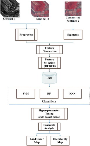
Hangzhou is comprised of 10 districts, one county-level city, and two counties and is the capital and most populous city of Zhejiang Province, People’s Republic of China. The region sits at the head of Hangzhou Bay in Eastern China, which separates Shanghai and Ningbo. Eight urban districts were selected as the study area, as shown in Figure 1: Shangcheng, Xiacheng, Gongshu, Binjiang, Jianggan, Yuhang, Xihu, and Xiaoshan. The climate in Hangzhou is humid subtropical with four distinctive seasons characterized by long, hot, humid summers and chilly, cloudy, dry winters (with occasional snow). The classification scheme from GlobeLand30 (Chen et al. 2015) was adopted and modified by removing some absent classes in Hangzhou, such as tundra, permanent snow, and ice. The main executed steps are summarized in the flowchart presented in Figure 2 and described in the following subsections.

Figure 1. Study area, Hangzhou city, is situated in the estuary of Qiantang River, eastern coastline of China. The major roads are displayed as red lines and topography are displayed using gray shades.

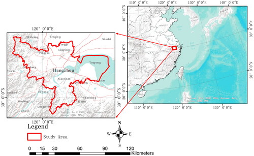
Figure 2. Schematic workflow chart of the proposed classification process.

2.1. Image preprocessing

Twenty-six Sentinel-1 images (–24 in ascending orbit and two in descending orbit) together with −27 Sentinel-2 images were selected as the input data based on the criteria given in Table 1. The images obtained from Sentinel-1 in the Google Earth Engine (GEE) were preprocessed using the Sentinel-1 toolbox. The preprocessing steps are: (1) thermal noise removal; (2) radiometric calibration; (3) terrain correction using SRTM 30 or ASTER DEM for areas greater than 60 degrees latitude when the SRTM is not available; and (4) the final terrain-corrected values are converted to decibels via log scaling [10*log10(x)]. The Sentinel-2 images were computed by running the sen2cor program. We used the three QA bands present in the Sentinel-2 images to indicate the presence of cloud and cloud shadows that mask invalid pixels. The mean values of the four spectral bands with a spatial resolution of 10 m were computed from the stack of cloud-free Sentinel-2 images and used as the inputs to the eCognition 9.0 software to generate the segments.

Table 1. Image selection criteria.

	Sentinel-1	Sentinel-2
Periods	(2019-05-01, 2019-09-30)	(2019-06-01, 2019-09-30)
Bounds	Administrative Boundary of Hangzhou
Cloudy Pixels	–	< 15%
Acquisition Mode	IW	–
Processing Level	GRD	Level-2A
Relative Orbit Number	Asc: 69, Desc: 3	–
Number of Images	Asc: 24, Desc: 2	27

2.2. Segmentation

We used the well-established multi-resolution image segmentation approach implemented in eCognition as it commonly achieves the best results compared with other algorithms (Myint et al. 2011). Several key parameters of the algorithm that need to be assigned appropriate values are the scale, shape, compactness, and weights of the bands. It is noted that though some tools (e.g. Automated Estimation of Scale Parameter Tool) enable automatic determination of optimal parameters for segmentation (Drăguţ et al. 2014), we stick to trial-and-error approach to determine optimal parameters, which allows us to make full use of local experience and expert knowledge about study area. Therefore, we used the trial-and-error approach, which is frequently applied in research, to determine the optimal scale. After the multi-scale segmentation algorithm is completed, the maximum spectral difference algorithm is applied to merge the over-split segments with a user-defined spectral difference threshold. This threshold is set to 2 so that spatially adjacent segments with spectral differences smaller than 2 are considered as homogeneous and merged.

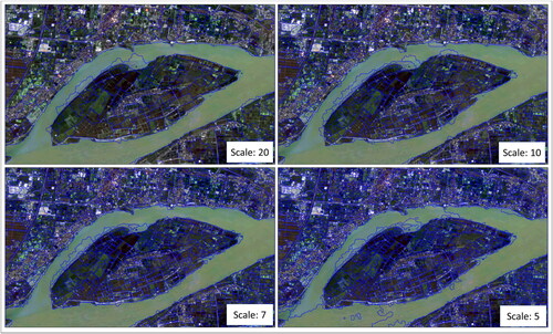
Based on the experimental results, the best segmentation was achieved with a scale of 7 when small objects (e.g. ponds) were identified and boundaries of large objects (e.g. rivers and villages) were delineated. The shape and compactness were set to 0.7 and 0.3, respectively. More emphasis was given to the shape than the spectral information to better preserve the natural boundaries of roads and rivers, where geometric features are good predictors. The weights for bands 2, 3, 4, and 8 were 1, 1, 1, and 2, respectively. The reason band 8 had a higher weight is that the near-infrared band is less correlated with the visible bands, which are highly correlated with each other (Figure 3).

Figure 3. Segmentation examples with different scale values.

2.3. Feature generation

The NDVI (Rouse et al. 1974) and normalized difference water index (NDWI) (Gao 1996), which were designed specifically to enhance the extraction of certain land cover classes, were computed from the composite cloud-free Sentinel-2 images. Their expressions are given as: (1) $$\mathrm{NDVI}=(B8-B4)/(B8+B4)$$(1) (2) $$\mathrm{NDWI}=(B3-B8)/(B3+B8)$$(2) where B3, B4, and B8 represent the third, fourth, and eighth bands of the Sentinel-2 images. The texture features, measured by the gray level concurrence matrix (GLCM), were computed using the wrapped GLCM function as implemented in GEE. The input image, which included the temporally averaged near-infrared band of Sentinel-2 and the VV and VH bands of Sentinel-1, was re-scaled to cover the 16-bit integer range. As suggested by (Stromann et al. 2019), the window size of neighborhood for calculating GLCM is set to 4, and GLCM in four directions ((−1, −1), (0, −1), (1, −1), and (−1, 0)) were calculated and averaged. The outputs are listed in Table 2. For a detailed description of the metrics, readers are referred to (Haralick et al. 1973; Conners et al. 1984).

Table 2. GLCM texture metrics.

Band	Description	Band	Description
contrast	contrast	var	sum of squares: variance
savg	sum average	sent	sum entropy
dvar	difference variance	imcorr1/2	information measures of correlation 1/2
inertia	inertia	asm	angular second moment
corr	correlation	idm	inverse difference moment
svar	sum variance	ent	entropy
dent	difference entropy	diss	dissimilarity

The input layers, such as the bands from the Sentinel-1/2, were aggregated into segments, and the common statistics (mean, max, min, and standard deviation) were calculated. The temporal standard deviation of the Sentinel-1 backscatter bands (VV and VH) in descending orbit was not calculated because there were only two acquisitions (Table 1). Thus, the temporal standard deviation would contain minimal information. Besides, 12 features in the geometric domain were generated from three shapes fit to the segments. In total, 568 features were generated, as shown in Table 3.

Table 3. Overview of all generated features.

Sensor	Input Layers	Segment Statistics (Mean, Min, Max, Std. Dev)	Number of Features
Sentinel-1	temporal mean	4 img (Asc/Desc, VV/VH)	16
	temporal std dev	2 img (Asc, VV/VH)	8
	texture features	6 img * 17 GLCM	408
Sentinel-2	cloud-free composites	12 spectral bands	48
		NDWI, NDVI	8
	NIR 10m band	17 GLCM	68
Geometry	Fitting Shape	Features	Number of Features
	min enclosing circle	radius, areal difference	2
	min area rotated rectangle	height, width, angle, aspect ratio, and areal difference	5
	least-squares-fit ellipse	major-axis, minor-axis, angle, aspect ratio, and areal difference	5
		SUM	568

2.4. Feature selection

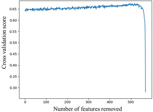
The ‘curse of dimension’ (G. Hughes 1968) is often encountered in classification tasks when there are too many features. If high-importance features are selected as a subset to build the model, the dimension problem will be greatly alleviated. Feature selection methods can be divided into three categories: filter, wrapper, and embedded techniques. The recursive feature elimination (RFE), which is a wrapper feature selection method, has been widely used to select features as derived from remotely sensed data (Pal and Foody 2010; Ma et al. 2017). Given an external estimator that assigns weights to features, the RFE selects features by recursively considering increasingly smaller feature sets. First, the estimator is trained on the initial set of features to obtain their relative importance. Then, the least important feature is pruned from the current set. This procedure is recursively repeated on the pruned feature set until the final feature is pruned. In this study, we used the random forest as the external estimator to calculate the overall accuracy with out-of-bag samples for each iteration. The initial feature set (568 features) and labeled samples were input into the random forest-based RFE function, and the overall accuracy was calculated using a 3-fold cross-validation. As shown in Figure 4, as the number of features decreased, the overall accuracy improved slowly with some initial fluctuations before rapidly decreasing. The highest overall accuracy was achieved for 53 features.

Figure 4. The number of features vs the cross-validation score.

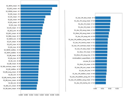
The 53 features were ranked based on their decreasing mean accuracy as evaluated using the random forest (Figure 5). It is noted that there is a defect in this ranking method as the correlation between features is not considered, which results in over-estimating the importance of relevant features. It is seen that eight out of the top 10 most important features come from Sentinel-2, because our definition for different land cover categories or classification schemes is based primarily on the characteristics obtained from optical imagery.

Figure 5. Histogram of feature importance where the label indicates the importance rank (the left shows the features from the Sentinel-2, and the right shows those from elsewhere).

2.5. Classification

Three machine learning algorithms are described in the following subsections. To achieve a better performance, some of the key hyper-parameters for each classifier need to be tuned and were determined using an exhaustive grid search with cross-validation. The candidates of the hyper-parameters and the corresponding model performance are shown in Figures 6–8.

Figure 6. Grid searching results for the hyper-parameters of the SVM. The optimal parameters are 0.1 and 10.0 for Gamma and C, respectively.

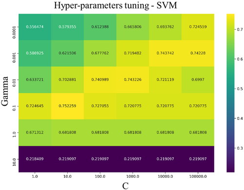
Figure 7. Grid searching results for the hyper-parameters of the RF. The optimal parameters are 9 and 800 for mtry and ntree, respectively.

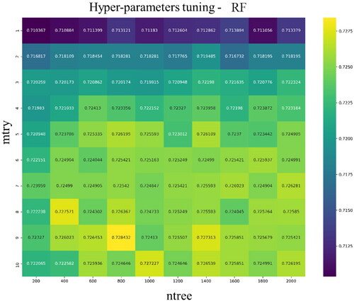
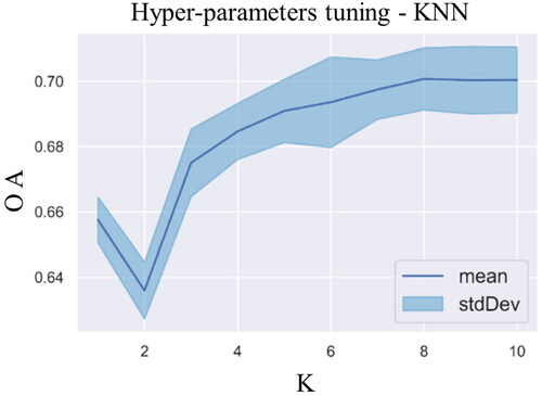
Figure 8. Grid searching results for the hyper-parameters of the KNN. The optimal parameter is 8 for K.

2.5.1. Support vector machine

In contrast to the parameterization classification, which characterizes the feature space for each class, the SVM considers only the samples, called support vectors, that are near the decision boundary between classes (Cortes and Vapnik 1995; Huang et al. 2002; Pal and Mather 2005). For linearly separable datasets, the goal of the SVM is to find the separation that has the widest buffer zone margin between two classes. For linearly inseparable datasets, one approach is to find a ‘soft-margin’ that allows some points to violate the constraints to some extent as captured by the slack variable. Another approach is to map the dataset to a higher dimensional feature space using kernel tricks (Kavzoglu and Colkesen 2009). The well-known kernel for remotely sensed datasets called the radial basis function (RBF) (Huang et al. 2002) was used here. Two key parameters for the RBF-based SVM are the C and gamma. The C parameter, which is the price of slackness, trades the classification correctness against the maximization of the decision boundary margin (Cortes and Vapnik 1995). A larger C usually indicates a smaller margin. The gamma parameter defines the reach for the influence of a single training sample, with a high value indicating ‘close’ and low meaning ‘far.’

2.5.2. Random forest

The RF is an ensemble algorithm that uses a large number of decision trees to overcome the disadvantages of a single decision tree, such as over-fitting and under-fitting problems (Breiman 2001; Pal 2005; He et al. 2017). The predictions for all decision trees are averaged using the majority vote rule to provide a globally optimal prediction. As indicated by its name, randomness is included in two steps: selecting samples to build each tree and selecting features to split each node in a tree. The unused samples rebuilding trees, also called out-of-bag (OOB) samples, can be used to estimate internal errors and measure the variable importance. Two important parameters to implement RF are the number of trees (ntree) and the number of features in each split (mtry).

2.5.3. K-nearest neighbors

The KNN classifier is different from others as it is not trained on labeled samples. Instead, the labeled samples are stored in the learning process of the model. The rationale behind the KNN is that it finds a group of k samples for the calibrated training data that are closest to the unlabeled samples in the feature space. The most common label for these k samples is assigned to the unlabeled sample (N. S. Altman 1992; Maselli et al. 2005). The key parameter of the classifier is k, where a lower value produces more complex decision boundaries, and larger values increase the model’s generalization but require more resources to store and index the training dataset.

2.6. Ensemble analysis

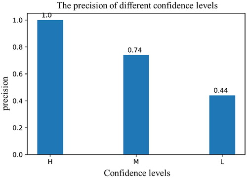
After the three primitive results were produced using the KNN, SVM, and RF, an ensemble analysis was employed to generate the final land cover map from each. Ensemble methods use multiple learning algorithms to obtain better predictive performances than from any of the constituent learning algorithms alone (Du et al. 2012). The majority vote, which is one of the easiest strategies to combine the outputs of several classifiers, assigns equal weights to each classifier and adopts the prediction with the most votes. This approach has the disadvantage that all the classifiers have equal rights to vote without considering their performances in each class. This could be mitigated by weighting the decisions from each classifier based on their accuracies obtained from the training data. The combination of the majority vote and accuracy-based weighting strategy has been widely adopted in combining outputs from three classifiers (Zhang 2015; Zhang et al. 2016), so it is adopted here. On an unknown sample, three classifiers may reach full, partial, or no agreement. In the first, second, and third situations, the samples are assigned the ‘agreed’ label with high confidence, the ‘partially agreed’ label with medium confidence, or the label given by the most accurate classifier, such as the KNN votes class 1, SVM votes class 2, and RF votes class 3. Class 3 is adopted if the RF has the highest accuracy among the KNN, SVM, and RF in identifying class 1, class 2, and class 3, respectively. Consequently, the uncertainty map is produced in conjunction with the final land cover map from the ensemble analysis. To verify whether the uncertainty map can provide insight into the spatial distribution of the error, we randomly selected 100 samples from each confidence level to assess the classification accuracy.

2.7. Accuracy assessment

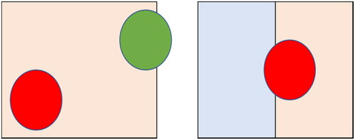
We generated 4,000 random points with a buffer of 10 m (circles) in the study area. These points were labeled by two interpreters with reference to the very-high resolution images of Google Earth. The class of an object was determined by the circle that has largest intersection area with it. For example, the object is assigned the class of the red circle in the left panel of Figure 9 as it has the largest intersection area with the object. The majority of the circle should lie in the object, otherwise, the object cannot be assigned the class of the circle. For example, the left object in the right panel of Figure 9 is not assigned as it contains less than half of the circle while the right object is assigned.

Figure 9. Illustration of how to assign the class of a random point to an object. For simplicity, the objects were abstracted as rectangles.

We determined the quality of the labeled objects, deleted incorrectly labeled objects, and added additional labeled objects into the minority class (e.g. roads). The labeled objects, or samples, were used to train and test the models. We then performed a three-fold cross-validation analysis using the labeled samples. The labeled samples were randomly divided into three groups of equal size. One group was used to assess the performance while the other two were used to train the classifier. This process was repeated three times to reduce the impact of variations in the samples splitting on accuracy. The final result is the average of the three primitive results. The metrics used to evaluate the map were the user accuracy (UA), producer accuracy (PA), and overall accuracy (OA).

2.8. Comparison experiments

2.8.1. Scenario design

We designed a four-scenario comparison experiment to demonstrate the added value to the proposed approach relative to traditional approaches that use single-data sources or single-temporal double-data sources (Table 4). To avoid the impact of segmentation on the classification accuracy, we used the same segmentation results from section B and extracted their geometric features. To reduce the impact of the acquisition time in scenario 1 in the classification accuracy, we used the temporal mean value image as calculated from the stack of cloud-free Sentinel-2 images instead of arbitrarily selected images. The temporal statistics (max, min, and standard deviation) for each band were added in scenario 2 and compared to scenario 1. The features derived from the SAR imagery were added in scenario 3 and compared to scenario 2. In scenario 4, the subset of features that were selected in subsection D was used. The features for the different scenarios were used as inputs to the random forest, which utilized 500 trees and the square root of the total number of features as the number of features for the splitting nodes.

Table 4. Data used in the four scenarios.

Scenario	Data
1	mono-temporal optical data
2	multi-temporal optical data
3	multi-temporal optical + SAR data
4	multi-temporal optical + SAR data (selected features)

2.8.2. Cross-validation paired t-test

The K-fold cross-validation paired t-test procedure is a common method to compare the performances of two models. For instance, models A and B are compared based on their predictions on the same labeled dataset. The k-fold cross-validation accuracies are then ${ϵ}_1^A,$ ${ϵ}_2^A,$…, ${ϵ}_k^A$ and ${ϵ}_1^B,$ ${ϵ}_2^B,$ …, ${ϵ}_k^B,$ where ${ϵ}_i^A$ and ${ϵ}_i^B$ indicate the accuracies of models A and B as obtained from the kth fold. Then, the difference between ${ϵ}_i^A$ and ${ϵ}_i^B$ is calculated as ${\Delta }_i={ϵ}_i^A-{ϵ}_i^B.$ If the performances of the two models are identical, the average of the difference ${\Delta }_i$ (i = 1, 2, …, k) should equal to zero. Thus, the naught hypothesis that model A performs equally well with model B is equivalent to the mean value of the sequence, ${\Delta }_1,$ ${\Delta }_2,$ …, ${\Delta }_k,$ being zero. We calculated the mean µ and the variance ${\mathrm{\sigma }}^2$ from the sequence and performed a t-test. For the statistical significance level of $\mathrm{\alpha },$ if the variable $${\mathrm{\tau }}_t=\left|\frac{\sqrt{k}\mathrm{\mu }}{{\mathrm{\sigma }}^2}\right|$$ is smaller than the threshold $t_{\alpha /2, k-1},$ the naught hypothesis cannot be rejected; else, the naught hypothesis is rejected. The $t_{\alpha /2, k-1}$ is the critical value for the cumulative distribution of $\mathrm{\alpha }/2$ in the tail of the t distribution with l-1 degrees of freedom.

3. Results

3.1. Visual analysis of results

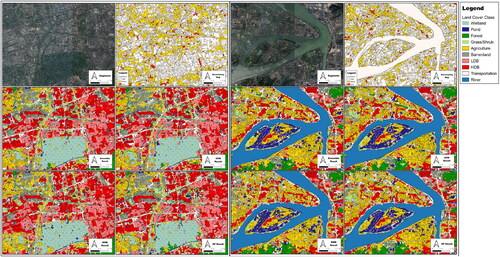
The legend of the land cover map (Figure 10a) and the magnified view of the results in urban (Figure 10b) and in rural (Figure 10c) areas are shown below. The images from left to right and from top to bottom are the very-high resolution base map from Google Earth, the uncertainty map, the ensemble analysis result, The SVM result, the KNN result, and the RF result.

Figure 10. Magnified view of results in urban (left) and rural (right). It shows image segmentation result, uncertainty map and four classification results.

3.2. Accuracy assessment

Shown below are the confusion matrices for the different classifiers in Figure 11, the producer and user accuracies for the outputs of the three classifiers in Table 5, and overall accuracy are in Table 6. The grass and shrubland class (G&S) achieved the lowest accuracy among the four results as suggested by their confusion matrices. A large proportion of the error was due to the misclassification of agricultural lands. A detailed inspection of land cover maps reveals that the main cause of the errors for the G&S was the spatial co-occurrence of the G&S and agricultural land (Figure 12). Agricultural lands are fragmented and separated by grass/shrubs, causing the G&S objects to be a mixture of G&S and agriculture lands. Even by visual inspection, it is difficult to distinguish between these categories. These problem areas tend to be low confidence regions in the uncertainty map, as shown in Figure 10.

Figure 11. Confusion matrices for the three base classifiers and the ensembled analysis.

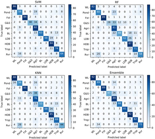
Figure 12. Spatial co-occurrence of grass and shrubland and agricultural land.

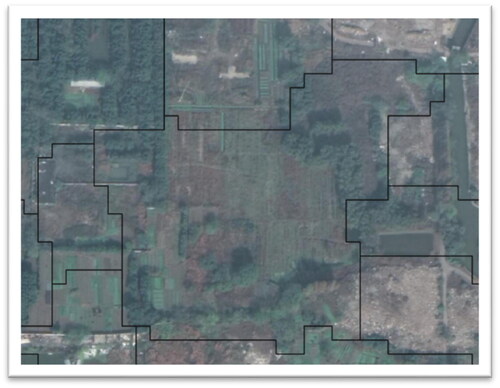
Table 5. Precision and recall of the base classifiers.

	Precision (UA)			Recall (PA)
class	SVM	RF	KNN	SVM	RF	KNN
WL	0.815	0.851	0.673	0.857	0.818	0.883
Pond	0.609	0.611	0.551	0.577	0.598	0.557
Forest	0.931	0.899	0.944	0.838	0.888	0.850
G&S	0.700	0.614	0.605	0.380	0.293	0.250
Agri	0.712	0.690	0.651	0.823	0.815	0.763
BL	0.598	0.568	0.605	0.632	0.483	0.529
LDB	0.731	0.710	0.653	0.681	0.611	0.681
HDB	0.810	0.778	0.783	0.839	0.867	0.853
Trsp	0.721	0.698	0.705	0.740	0.719	0.694
River	0.681	0.682	0.733	0.640	0.600	0.440

Table 6. OA of the classifiers.

	SVM	RF	KNN	Ensemble
OA	0.738	0.717	0.699	0.816

3.3. Uncertainty map assessment

We randomly selected 100 samples from each level to evaluate the classification accuracy of different confidence levels in the uncertainty map, as shown in Figure 13. The precisions for the high, medium, and low levels are 100%, 74%, and 44%, respectively. To further improve the accuracy of the land cover map, manual editing of misclassified samples in post-classification is necessary. As demonstrated that the uncertainty map is a useful tool to visualize the error-prone area, researchers can save a lot of time by focusing only on samples from low and medium levels.

Figure 13. The precision for different confidence levels.

3.4. Comparison analysis

The ‘i/j’ in the parenthesis of the ${\mathrm{\tau }}_{\mathrm{t}}$ column in Table 7 indicates the paired t-test result between scenario i and scenario j, while the ‘*’ and ‘**’ indicate the statistical significance for the 95% and 99% confidence levels. It is seen that the differences in the OA between scenarios are all statistically significant at the 99% level except for ‘1/2,’ which is statistically significant at the 95% level. The overall accuracies of the four scenarios and their associated standard deviations are shown in Figure 14. The overall accuracies increase from scenario 1 to scenario 3 as a result of the additional information in the temporal and polarimetric dimensions. At the same time, the standard deviation increases because additional noise and low-information features are inevitably included. Feature selection was performed in scenario 4 and compared with scenario 3, which led to not only an increased overall accuracy but also a decrease in the standard deviation. Another implicit advantage is that the computational burden was significantly reduced as the number of features decreased from around 600 to 53.

Figure 14. The overall accuracies and associated standard deviations for the four scenarios.

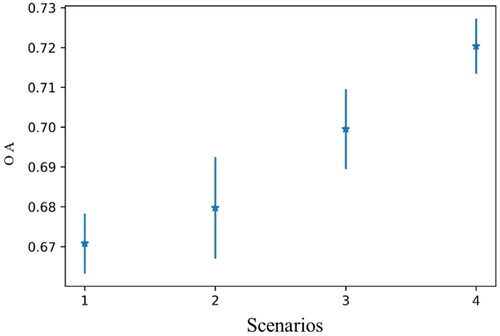
Table 7. The OA, and ${\mathrm{\tau }}_{\mathrm{t}}$ for the four scenarios.

Scenario	OA	${\mathbf{\tau }}_{\mathbf{t}}$
1	0.671	2.615*, 8.99**, 16.757** (1/2, 1/3, 1/4)
2	0.680	6.588**, 12.394** (2/3, 2/4)
3	0.700	15.025** (3/4)
4	0.720	–

4. Discussion

The development of new generation of satellite remote sensing missions leads to big data of Earth observation from different sensors, with improved spatial, temporal, and spectral resolutions. In parallel, greater computing power provided by cloud computing technology is also enabling scientists to manipulate these data to map land cover in a timely and accurate manner. Image processing methodologies are also critical to the improvement of performance, including object-based image analysis, feature engineering and ensemble analysis.

4.1. Object-based image analysis

As fine resolution imagery is increasingly accessible, evolving object-based image analysis has demonstrated preeminence over the traditional pixel-based approach and enable the utilization of diverse spectral, geometrical, and texture information for image classification (Hamedianfar et al. 2022). Besides, object-based classification decreases the computational load, because the number of units to be classified are dramatically reduced after aggregating pixels into objects. Although image segmentation in GEE, currently, is limited to non-iterative clustering algorithm (Shafizadeh-Moghadam et al. 2021) and simple connected pixel neighborhood analysis (Xiao et al. 2021), it can be done outside GEE; the results are then uploaded to GEE for subsequent processing. We integrate the image segmentation algorithm implemented in eCognition into our work flow, because it provides wealth of sophisticated image segmentation algorithms. It should be noted that that trial-and-error approach for threshold offers us flexibility in tuning result at local study, but may not suitable for large-scale studies.

4.2. Feature engineering

Feature engineering is the process of selecting, manipulating, and transforming raw data into features that can be used in supervised learning. A variety of features can be generated from multi-temporal, multi-sensor images and object-based image analysis. ESA World Cover product extracts 12 features from Sentinel-1, 64 features from Sentinel-2, 2 features from digital elevation models, 23 positional features and 14 meteorological features, for a total of 115 features (Zanaga et al. 2022). Feature selection involves considerable expert knowledge. In the absence of such knowledge, random forest can be used to measure feature importance to exclude less important features (Shafizadeh-Moghadam et al. 2021). It is noted that the importance ranking of features is affected by the design of the classification scheme. For example, when classification tends to divide different categories based on texture features in SAR images, the importance of texture features increases. As the design of classification schemes varies depending on goal of land cover map, data source, and landscape of the research area, the automatic selection for an optimal subset of features is useful. The necessity of feature selection was demonstrated by comparing scenarios 3 and 4. In previous study (Schulz et al. 2021), RF performed best with the full number of features, while the application of feature selection in our case resulted in a nearly 2% increase in the overall accuracy with RF, breaking theory-based expectations regarding low sensitivity to overfitting. It can be explained by extreme redundancy and collinearity among nearly 600 features. In (Paul and Kumar 2019), it is found that feature extraction techniques result in better performance compared to feature selection approaches when multi-temporal datasets are employed to map crop types. It’s worth comparing different feature reduction techniques in urban land cover mapping.

4.3. Ensemble learning

Ensemble learning combines a series of good and diverse base classifiers to achieve better performance. Random forests combine arrays of tree predictors such that each tree depends on the values of a random vector sampled independently and with the same distribution for all trees in the forest (Breiman 2001). While most studies employed RF to map land covers (Cao et al. 2021; Du et al. 2021; Zhang et al. 2021; Castro et al. 2022), a few studies further ensembled RF with other classifiers, aiming to improve mapping. Schulz et al. (2021) ensembled RF with maximum likelihood classifier and SVM for mapping heterogeneous landscape in Niger, Sahel. It was found that performance was improved in terms of accuracy, particularly with respect to built-up areas. Chen et al. (2021) proposed an ensemble learning framework that leveraged RF, CatBoost, LightGBM and neural networks to map essential urban land use categories in five metropolitan areas in the United States of America. Our study also finds that ensemble analysis produces better results compared with using single classification algorithm.

5. Conclusions

We performed object-based land cover classification using multi-temporal Sentinel-1/2 images based on the Google cloud platform with promising results. Nearly 600 features in the spectral, polarimetric, spatial, temporal, and geometric dimensions were generated from stacks of Sentinel-1/2 images. Then, the random forest algorithm based on the recursive feature elimination method was performed to find that the optimal subset of features, totaling 53. The importance of the selected features was estimated using the random forest. The selected subset of features was used as the input to the SVM, RF, and KNN, whose hyper-parameters are well-tuned using the training dataset with cross-validation. The outputs of the three classifiers were the basis of the ensemble analysis. The ensemble analysis produced improved results with the accompanying uncertainty map. The uncertainty map indicates potential problematic areas and was validated using an accuracy assessment with the stratified sampling strategy. Accuracies of the high, medium, and low confidence groups were 100%, 74%, and 44%, respectively. In the comparison experiment, four scenarios that used different data were designed to demonstrate the advantages of the multi-temporal synergy of the optical and SAR data compared with traditional approaches that only use optical data. The application of feature selection also played an important role in enhancing the classification accuracy with an approximately 2% increase in the overall accuracy, which was observed apart from the reduced computation burden and standard deviation of the accuracy.

Disclosure statement

No potential conflict of interest was reported by the author(s).

Additional information

Funding

This research was supported by the Key R&D Program of Zhejiang Province (2022C03154) and Natural Science Foundation of Zhejiang Province (LY20D010008).

References

- Almeida Cd, Coutinho AC, Esquerdo JCDM, AdamiI M, Venturieri A. 2016. High spatial resolution land use and land cover mapping of the Brazilian Legal Amazon in 2008 using Landsat-5/TM and MODIS data. Acta Amaz. 46:291–302.
- Altman NS. 1992. An introduction to Kernel and nearest-neighbor nonparametric regression. Am Stat. 46:175–185.
- Ban Y, Hu H, Rangel IM. 2010. Fusion of Quickbird MS and RADARSAT SAR data for urban land-cover mapping: object-based and knowledge-based approach. Int J Remote Sens. 31:1391–1410.
- Breiman L. 2001. Random forests. Machine Learning. 45:p. 5–32.
- Brown CF, Brumby SP, Guzder-Williams B, Birch T, Hyde SB, Mazzariello J, Czerwinski W, Pasquarella VJ, Haertel R, Ilyushchenko S, et al. 2022. Dynamic World, Near real-time global 10 m land use land cover mapping. Sci Data. 9:1–17. https://www.nature.com/articles/s41597-022-01307-4.
- Cao B, Yu L, Naipal V, Ciais P, Li W, Zhao Y, Wei W, Chen D, Liu Z, Gong P. 2021. A 30 m terrace mapping in China using Landsat 8 imagery and digital elevation model based on the Google Earth Engine. Earth Syst. Sci. Data. 13:2437–2456. English. https:// essd.copernicus.org/articles/13/2437/2021/.
- Castro P d, Yin H, Teixera Junior PD, Lacerda E, Pedroso R, Lautenbach S, Vicens RS. 2022. Sugarcane abandonment mapping in Rio de Janeiro state Brazil. Remote Sens Environ. 280:113194. https://www.sciencedirect.com/science/article/pii/S0034425722003042.
- Chen J, Chen J, Liao A, Cao X, Chen L, Chen X, He C, Han G, Peng S, Lu M, et al. 2015. Global land cover mapping at 30m resolution: a POK-based operational approach. ISPRS J Photogramm Remote Sens. 103:7–27. https://www.sciencedirect.com/science/article/pii/S0924271614002275.
- Chen B, Tu Y, Song Y, Theobald DM, Zhang T, Ren Z, Li X, Yang J, Wang J, Wang X, et al. 2021. Mapping essential urban land use categories with open big data: results for five metropolitan areas in the United States of America. ISPRS J Photogramm Remote Sens. 178:203–218. https://www.sciencedirect.com/science/article/pii/S0924271621001684.
- China Statistical Yearbook. 2019. 2019. [S.l.]: CHINA STATISTICS PRESS. ISBN: 9787503788970.
- Conners RW, Trivedi MM, Harlow CA. 1984. Segmentation of a high-resolution urban scene using texture operators. Computer Vision, Graphics, and Image Process. 25:273–310.
- Corbane C, Faure J-F, Baghdadi N, Villeneuve N, Petit M. 2008. Rapid urban mapping using SAR/optical imagery synergy. Sensors (Basel). 8(11):7125–7143. https://www.mdpi.com/1424-8220/8/11/7125.
- Cortes C, Vapnik V. 1995. Support-vector networks. Mach Learn. 20:273–297. https://link.springer.com/content/pdf/10.1007/BF00994018.pdf.
- Deus D. 2016. Integration of ALOS PALSAR and landsat data for land cover and forest mapping in Northern Tanzania. Land. 5:43. https://www.mdpi.com/2073-445X/5/4/43.
- Drăguţ L, Csillik O, Eisank C, Tiede D. 2014. Automated parameterisation for multi-scale image segmentation on multiple layers. ISPRS J Photogramm Remote Sens. 88(100):119–127. https://www.sciencedirect.com/science/article/pii/S0924271613002803.
- Du P, Xia J, Zhang W, Tan K, Liu Y, Liu S. 2012. Multiple classifier system for remote sensing image classification: a review. Sensors (Basel). 12(4):4764–4792.
- Du Z, Yang J, Ou C, Zhang T. 2021. Agricultural land abandonment and retirement mapping in the Northern China crop-pasture band using temporal consistency check and trajectory-based change detection approach. IEEE Transact Geosci Remote Sens. 60(1):1-12.
- Franklin SE, Peddle DR. 1990. Classification of SPOT HRV imagery and texture features. Remote Sens. 11(3):551–556.
- Friedl MA, Sulla-Menashe D, Tan B, Schneider A, Ramankutty N, Sibley A, Huang X. 2010. MODIS Collection 5 global land cover: algorithm refinements and characterization of new datasets. Remote Sens Environ. 114(1):168–182. http://www.sciencedirect.com/science/article/pii/S0034425709002673.
- Gao B-c. 1996. NDWI—A normalized difference water index for remote sensing of vegetation liquid water from space. Remote Sens Environ. 58(3):257–266.
- Hamedianfar A, Gibril MBA, Hosseinpoor M, Pellikka PKE. 2022. Synergistic use of particle swarm optimization, artificial neural network, and extreme gradient boosting algorithms for urban LULC mapping from WorldView-3 images. Geocarto Int. 37(3):773–791.
- Haralick RM, Shanmugam K, Dinstein IH. 1973. Textural features for image classification. IEEE Trans Sys Man Cybernet. SMC-3(6):610–621.
- He Y, Lee E, Warner TA. 2017. A time series of annual land use and land cover maps of China from 1982 to 2013 generated using AVHRR GIMMS NDVI3g data. Remote Sens Environ. 199:201–217. http://www.sciencedirect.com/science/article/pii/S0034425717303255.
- Huang C, Davis LS, Townshend JRG. 2002. An assessment of support vector machines for land cover classification. Int J Remote Sens. 23(4):725–749.
- Hughes G, G 1968. On the mean accuracy of statistical pattern recognizers. IEEE Trans. Inform. Theory. 14(1):55–63.
- Jhonnerie R, Siregar VP, Nababan B, Prasetyo LB, Wouthuyzen S. 2015. Random forest classification for mangrove land cover mapping using landsat 5 TM and Alos Palsar imageries. Procedia Environ Sci. 24:215–221. http://www.sciencedirect.com/science/article/pii/S1878029615000961.
- Kavzoglu T, Colkesen I. 2009. A kernel functions analysis for support vector machines for land cover classification. Int J Appl Earth Obs Geoinf. 11(5):352–359. http://www.sciencedirect.com/science/article/pii/S0303243409000464.
- Krishna Karra C, Kontgis Z, Statman-Weil JC, Mazzariello M, Mathis S, Brumby. 2021. Global land use/land cover with Sentinel 2 and deep learning. 2021 IEEE International Geoscience and Remote Sensing Symposium IGARSS. https://www.semanticscholar.org/paper/Global-land-use-%2F-land-cover-with-Sentinel-2-and-Karra-Kontgis/0867e552c141208e6af89184fc61b9d0e494b965.
- Ma L, Fu T, Blaschke T, Li M, Tiede D, Zhou Z, Ma X, Chen D. 2017. Evaluation of feature selection methods for object-based land cover mapping of unmanned aerial vehicle imagery using random forest and support vector machine classifiers. IJGI. 6(2):51. https://www.mdpi.com/2220-9964/6/2/51/pdf.
- Ma L, Liu Y, Zhang X, Ye Y, Yin G, Johnson BA. 2019. Deep learning in remote sensing applications: a meta-analysis and review. ISPRS J Photogramm Remote Sens. 152:166–177.
- Maselli F, Chirici G, Bottai L, Corona P, Marchetti M. 2005. Estimation of Mediterranean forest attributes by the application of k‐NN procedures to multitemporal Landsat ETM + images. Int J Remote Sens. 26(17):3781–3796.
- Myint SW, Gober P, Brazel A, Grossman-Clarke S, Weng Q. 2011. Per-pixel vs. object-based classification of urban land cover extraction using high spatial resolution imagery. Remote Sens Environ;115:1145–1161. http://www.sciencedirect.com/science/article/pii/S0034425711000034.
- Pal M. 2005. Random forest classifier for remote sensing classification. Int J Remote Sens. 26(1):217–222.
- Pal M, Foody GM. 2010. Feature selection for classification of hyperspectral data by SVM. IEEE Trans Geosci Remote Sens. 48(5):2297–2307.
- Pal M, Mather PM. 2005. Support vector machines for classification in remote sensing. Int J Remote Sens. 26(5):1007–1011.
- Paul S, Kumar DN. 2019. Evaluation of feature selection and feature extraction techniques on multi-temporal landsat-8 images for crop classification. Remote Sens Earth Syst Sci. 2(4):197–207. https://link.springer.com/article/10.1007/s41976-019-00024-8.
- Pavanelli JAP, Santos J, Galvão LS, Xaud M, Xaud HAM. 2018. PALSAR-2/ALOS-2 and OLI/LANDSAT-8 data integration for land use and land cover mapping in Northern Brazilian Amazon. Bol Ciênc Geod. 24(2):250–269.
- Pereira LO, Freitas CC, SantaAnna SJS, Reis MS. 2018. Evaluation of optical and radar images integration methods for LULC classification in Amazon region. IEEE J Sel Top Appl Earth Observ Remote Sens. 11(9):3062–3074.
- Rouse JW, Haas RH, Schell JA, Deering DW. 1974. Monitoring vegetation systems in the Great Plains with ERTS. NASA Special Publication. 351:309.
- Schulz D, Yin H, Tischbein B, Verleysdonk S, Adamou R, Kumar N. 2021. Land use mapping using Sentinel-1 and Sentinel-2 time series in a heterogeneous landscape in Niger, Sahel. ISPRS J Photogramm Remote Sens. 178:97–111. https://www.sciencedirect.com/science/article/pii/S0924271621001635.
- Sentinel-1 - Missions - Sentinel Online. 2020. [place unknown]: [publisher unknown]; [updated 2020 May 14; accessed 2020 May 14]. https://sentinel.esa.int/web/sentinel/missions/sentinel-1.
- Sentinel-2 - Missions - Sentinel Online. 2020. [place unknown]: [publisher unknown]; [updated 2020 May 14; accessed 2020 May 14]. https://sentinel.esa.int/web/sentinel/missions/sentinel-2.
- Shafizadeh-Moghadam H, Khazaei M, Alavipanah SK, Weng Q. 2021. Google Earth Engine for large-scale land use and land cover mapping: an object-based classification approach using spectral, textural and topographical factors. GISci Remote Sens. 58(6):914–928.
- Stromann O, Nascetti A, Yousif O, Ban Y. 2019. Dimensionality reduction and feature selection for object-based land cover classification based on Sentinel-1 and Sentinel-2 time series using Google Earth Engine. Remote Sens. 12(1):76. https://www.mdpi.com/2072-4292/12/1/76/pdf.
- Torres R, Snoeij P, Geudtner D, Bibby D, Davidson M, Attema E, Potin P, Rommen B, Floury N, Brown M, et al. 2012. GMES Sentinel-1 mission. Remote Sens Environ. 120:9–24. http://www.sciencedirect.com/science/article/pii/S0034425712000600.
- Venter ZS, Barton DN, Chakraborty T, Simensen T, Singh G. 2022. Global 10 m land use land cover datasets: A comparison of dynamic world, world cover and Esri land cover. Remote Sens. 14(16):4101. https://www.mdpi.com/2072-4292/14/16/4101.
- Walter V. 2004. Object-based classification of remote sensing data for change detection. ISPRS J Photogramm Remote Sens. 58(3–4):225–238.
- Wolter PT, Mladenoff DJ, Host GE, Crow TR. 1995. Using multi-temporal landsat imagery. Photogramm Engin Remote Sens. 61:1129–1143.
- Xiao W, Xu S, He T. 2021. Mapping paddy rice with Sentinel-1/2 and phenology-, object-based algorithm—A implementation in Hangjiahu Plain in China using GEE platform. Remote Sens. 13(5):990.
- Zanaga D, van de Kerchove R, Daems D, Keersmaecker W, de Brockmann C, Kirches G, Wevers J, Cartus O, Santoro M, Fritz S, et al. 2022. ESA WorldCover 10 m 2021 v200. Europe: Zenodo. https://zenodo.org/record/7254221#.Y8VM2HZBxdA.
- Zanaga D, van de Kerchove R, Keersmaecker W d, Souverijns N, Brockmann C, Quast R, Wevers J, Grosu A, Paccini A, Vergnaud S, et al. 2021. ESA WorldCover 10 m 2020 v100.
- Zhang C. 2015. Applying data fusion techniques for benthic habitat mapping and monitoring in a coral reef ecosystem. ISPRS J Photogramm Remote Sens. 104:213–223.
- Zhang X, Liu L, Chen X, Gao Y, Xie S, Mi J. 2021. GLC_FCS30: global land-cover product with fine classification system at 30 m using time-series Landsat imagery. Earth Syst Sci Data. 13(6):2753–2776. https://essd.copernicus.org/articles/13/2753/2021/essd-13-2753-2021-discussion.html.
- Zhang C, Selch D, Cooper H. 2016. A framework to combine three remotely sensed data sources for vegetation mapping in the Central Florida everglades. Wetlands. 36(2):201–213. https://link.springer.com/article/10.1007%2Fs13157-015-0730-7.
- Zhang C, Smith M, Fang C. 2018. Evaluation of Goddard’s LiDAR, hyperspectral, and thermal data products for mapping urban land-cover types. GISci Remote Sens. 55(1):90–109.
- Zhu Z, Woodcock CE, Rogan J, Kellndorfer J. 2012. Assessment of spectral, polarimetric, temporal, and spatial dimensions for urban and peri-urban land cover classification using Landsat and SAR data. Remote Sens Environ. 117:72–82. http://www.sciencedirect.com/science/article/pii/S0034425711002823.