Sunflower crop yield prediction by advanced statistical modeling using satellite-derived vegetation indices and crop phenology

Abstract

Timely crop yield information is needed for agricultural land management and food security. We investigated using remote sensing data from the Earth observation mission Sentinel-2 to monitor the crop phenology and predict the crop yield of sunflowers at the field scale. Ten sunflower fields in Mezőhegyes, southeastern Hungary, were monitored in 2021, and the crop yield was measured by a combine harvester. Images from Sentinel-2 were collected throughout the monitoring period, and vegetation indices (VIs) were extracted to monitor the crop growth. Multiple linear regression and two different machine learning approaches were applied to predicting the crop yield, and the best-performing one was selected for further analysis. The results were as follows. The VIs showed the highest correlation with the crop yield (R > 0.6) during the inflorescence emergence stage. The most suitable time for predicting the crop yield was 86–116 days after sowing. Random forest regression (RFR) was the best machine learning approach for predicting field-scale variability of the crop yield (R² ∼ 0.6 and RMSE 0.284–0.473 t/ha). Our results can be used to develop a timely and robust prediction method for sunflower crop yields at the field scale to support decision-making by policymakers regarding food security.

Keywords:

• Support vector machine regression
• days after sowing
• precision agriculture
• spectral reflectance
• random forest regression

1. Introduction

The sunflower is an important oilseed crop native to South America that is currently cultivated in many countries around the world because of its nutritional and medicinal value (Adeleke and Babalola 2020). It plays a significant role in the cooking oil market because of its high level of unsaturated fatty acids and high smoke point, which are beneficial for human diets (OECD and Food and Agriculture Organization of the United Nations, 2016). Today, sunflowers are used for culinary purposes more than soybeans and rapeseed because of its high oil content (Pal et al. 2015). In the European Union (EU), Hungary is the second-largest producer of sunflowers after Romania with a harvest of 1.8 million tons in 2020. However, despite Hungary expanding the cultivation of sunflowers, its crop yield has decreased significantly since 2018. Timely and regular information about crop development and crop yield is necessary to prevent potential losses before harvesting (Szabó et al. 2019).

Remote sensing (RS) provides farmers and owners with important and necessary information for early crop yield prediction (Huang et al. 2013). RS and modern machine learning (ML) approaches can be used to predict crop yields at a low cost and with high precision (Wang et al. 2018). In agricultural research, satellite imagery facilitates the quick and inexpensive assessment of crop yields (Singh et al. 2002). Plants undergo physiological and morphological changes as they grow, which determine their phenological stages. By describing these phenological stages, known as growth stages, we can correlate them with the time that different environmental factors and management issues take place, making it easier to understand the responses of crops. Traditionally, ground-based monitoring is used to determine crop growth stages. These activities also require time and resources, suggesting that large-scale implementation is not common, despite their ability to provide accurate phenology analysis of crops. Satellite-based crop phenology monitoring through VIs enables tracking of timely positive and negative dynamics of crop development on crop health status. Phenology plays an important role in agricultural production, yield estimation, modeling surface energy-water-carbon fluxes, and managing farming practices (e.g. irrigation scheduling, fertilizer management, harvesting) (Lokupitiya et al. 2009; Bolton and Friedl 2013; Sakamoto et al. 2013). Due to seasonal differences in the biochemical and physiological characteristics of crops (e.g. light use efficiency), crops are managed by seasonal phenological development stages. Early crop yield prediction is important for ensuring food security, generating early warnings about field-scale variability in seed production, and ensuring reliable import and export flows (Khaki and Wang 2019).

RS-derived vegetation indices (VIs) are widely used for monitoring vegetation and crops (Jaafar and Ahmad 2015). Representative examples include the normalized difference vegetation index (NDVI), soil adjusted vegetation index (SAVI), enhanced vegetation index 2 (EVI 2), green normalized difference vegetation index (GNDVI), and normalized difference red edge (NDRE) (Tucker 1979; Huete 1988; Gitelson et al. 1996; Kayad et al. 2016; Xue and Su 2017). Since the late 1980s, NDVI has been the most widely used in agricultural research for crop growth monitoring and analysis (Panda et al. 2010). EVI 2 is also widely used in research on crop growth and yields, and it is based on the near-infrared and red regions of the electromagnetic spectrum. However, EVI is less sensitive than NDVI to different soil backgrounds (Shammi and Meng 2021). (Jin et al. 2016) showed that the normalized difference moisture index (NDMI) is strongly correlated to biomass with a reduced signal compared to that for dry matter. However, NDMI contains data at 1649 and 1722 nm, which are sensitive to changes in dry matter.

Various ML-based prediction models have been developed that use RS-derived VIs to predict crop yields at the regional and field scales (Andrianasolo et al. 2014; Wang et al. 2014; Fieuzal et al. 2017; Schwalbert et al. 2020; Trépos et al. 2020; Narin and Abdikan 2022). Trépos et al. (2020) combined a simulation model with the time series of the leaf area index (LAI) extracted from Sentinel-2A and Landsat 8 satellite images of 281 fields near Toulouse, France, to predict the sunflower crop yield. Their results showed that data assimilation significantly improved the prediction accuracy from a root mean square error (RMSE) of 988 kg/ha to 749 kg/ha. They also concluded that using a smoothed LAI rather than raw LAI improved the prediction performance. (Narin et al. 2021) investigated combining NDVI and NDVI red-edge (NDVIred) generated from Sentinel-2 satellite images with linear regression, a convolutional neural network (CNN), and artificial neural network (ANN) for predicting the sunflower crop yield of 48 fields in the Zile district of Tokat Province, Turkey. Their results showed that NDVI and NDVIred could be used to predict the crop yield at the field scale. The best prediction performance was obtained by combining NDVI and CNN, which resulted in an RMSE of 2,0874 kg/ha. Micheneau et al. (2017) used RS data and statistical models based on crop yield data provided by a commercial yield monitoring system to predict the crop yield of 187 sunflower fields in 2014 and 2015. Their approach combined the green area index (GAI) derived from Landsat 8 and Spot 5 products with linear, quadratic, linear-plateau, and quadratic with plateau models. They calculated two variables for crop yield prediction: maximum GAI (GAImax) and green area duration (GAD). Their results indicated that the crop yield could be accurately predicted 3 weeks before the harvesting stage. The best prediction performances were obtained by GAD or GAD + GAImax with RMSE < 400 kg/ha and R² = 0.44 for both years.

In the present study, we considered a small region with different field sizes, soil, and vegetation. Predicting the crop yield for such a study area would be very difficult owing to the wide variability in data. Thus, we developed a new approach based on pixel-by-pixel calculation statistics for the assessment and monitoring of crop yield and field-scale variability. Our main objective was to evaluate the potential of different RS-derived VIs for monitoring the field-scale variability in the sunflower crop yield when combined with different regression analysis techniques. The following research questions were set in this study:

1. Which time and crop age are suitable for predicting crop yield variability at the field scale?

2. Which ML technique is best for high-resolution wheat yield mapping using VIs from Sentinel-2 images?

2. Materials and methods

2.1. Study area

Mezhegyes, Békés County, in southeastern Hungary near the Romanian border (46°19′ N, 20°49′ E) is the study area, which included 10 sunflower fields (Figure 1). Five fields were used for training, and five fields were used for testing, also there is information about used parcels (Table 1). Mezőhegyes is a town with a total administrative area of 15,544 ha and a population of 4950 people. The soil in the meadows and lowlands is mostly chernozem, which is a very common soil type with high lime content that is excellent for agriculture, especially cereal and oilseed crops (Amankulova et al. 2021). The experimental farm at Mezőhegyes (Mezőhegyesi Ménesbirtok Zrt.) plays an important role in both Mezőhegyes and neighboring settlements.

Figure 1. Study area. (a) The areas highlighted with red colour indicate training fields and the blue colour represented test fields. (Natural colour composite from Sentinel-2 imagery; bands: RGB (4, 3, 2): acquisition date: 13th July 2021). Pictures showing the growing stage of the sunflower plant according to the dates on (b) 14 June and (c) July 30, 2021, in the field.

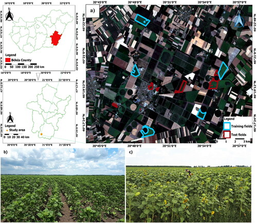
Table 1. Information about 10 sunflower fields.

Training areas			Test areas
N	Field number	Field size (ha)	N	Field number	Field size (ha)
1	Field 1	89.9	1	Field 1	79.5
2	Field 2	55.1	2	Field 2	4.1
3	Field 3	75.4	3	Field 3	8.2
4	Field 4	46.6	4	Field 4	46.6
5	Field 5	86.6	5	Field 5	18.1

2.2. Climate data

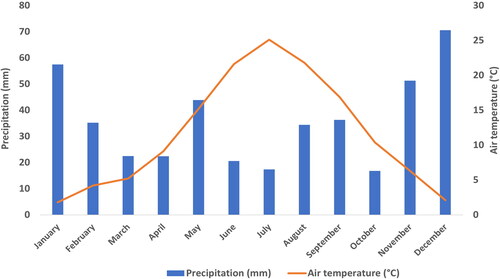
Meteorological datasets were downloaded for the 2021 year over the study site (Figure 2). The daily total rainfall (mm) and mean air temperature (°C) were obtained from the operational drought and water scarcity management system (OVF) (https://aszalymonitoring.vizugy.hu/, accessed February 15, 2022). According to OVF and the experimental farm at Mezőhegyes, the rainfall was 428.9 mm for the 2021 growing season (i.e. from planting to harvest). Climate records were obtained from Mezőhegyes station next to the selected fields.

Figure 2. Monthly precipitation and temperature at: Mezőhegyes Meteorological Station in 2021. (Data derived from http://aszalymonitoring.vizugy.hu).

2.3. Crop yield measurements

The sunflower is a common crop in Mezőhegyes. In 2021, fields were prepared for the seeding process on March 26, and sunflowers were sown on March 31 in 20 fields covering 1174.4 ha, which comprised almost 15% of the total area of the experimental farm. Chemicals were sprayed for weed control on May 7, followed by chemicals against insects and bacteria on June 29. No additional nutrients or irrigation was implemented to increase the crop yield during the growing season. At the end of the growing season, the sunflower crop was harvested with a John Deere W650i combine harvester on September 26. The combine harvester was equipped with a yield-mapping system with Green Star software that recorded crop yield data in a point shape format. Approximately one yield record was obtained every 2 s that could be viewed and manipulated in a geographic information system (GIS). Because no chemicals were used to speed up the growing season, the crop was harvested late, and the sunflower seeds were dried naturally. The average crop yield of the 10 fields was 4000 kg/ha. The crop yield data were filtered to remove outlier values (Kharel et al. 2019). Commercial yield monitors are prone to recording erroneous data when harvested rows overlap, which would suggest a low crop yield in specific areas of the field. Therefore, straight-line sequences of points that showed a near-zero yield were removed. Calibrated and filtered crop yield data were collected from the company that owns and manages farming operations in the study area. Only crop yield data with the same width and distance were left corresponding to the header dimensions of the combine harvester (i.e. 2 m × 6 m). We then converted the crop yield data to raster format by using the inverse distance weighted (IDW) interpolation method in QGIS v.3.16 with 10 m × 10 m pixels to match the resolution of the satellite images. We used this data as a response variable for the prediction models of the crop yield using RS-derived VIs.

2.4. Satellite imagery

Sentinel-2 Level 2 A (L2A) bottom-of-atmosphere (BOA) reflectance products were obtained from the Copernicus Open Access Hub website (https://scihub.copernicus.eu/dhus/#/home, accessed 1 September 2021). The overall workflow is illustrated in Figure 3. Sentinel-2 satellites carry a Multispectral Imager (MSI) that can measure 13 spectral bands at high spatial resolution: four bands at 10 m, six bands at 20 m, and three bands at 60 m (Appendix 1). Sixteen cloud-free satellite images were downloaded showing the various stages of the sunflower growing season from April to September 2021. The crop age was defined by the number of days after sowing (DAS) (Table 2). All images were resampled from different pixel sizes into a 10 m resolution using the Sentinel Application Platform (SNAP) version 8.0 (https://step.esa.int, accessed 15 February 2021) developed by the European Space Agency (ESA). We extracted the fields in the study area by using the official crop plan map as a mask layer in QGIS 3.16. We then created a grid rectangle (polygon) at 10 × 10 m to extract pixel values for model development to match the spatial resolution of the Sentinel-2 images.

Figure 3. Overall workflow adopted in this study.

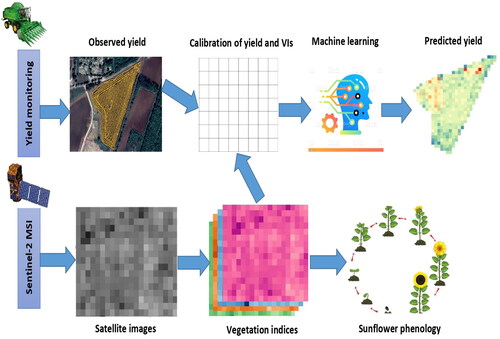
Table 2. Sentinel-2 images used in this study.

2021 Season
Planting Date: March 31, 2021 Harvesting Date: September 26, 2021
Date	DAS	Growing stage
April 9	9	Leaf Development
May 11	41
May 21	51
June 20	81	Stem Elongation
June 23	84
June 25	86
July 8	99	Inflorescence Emergence
July 13	106
July 25	116
July 30	121	Flowering
August 9	131
August 12	134	Ripening
August 14	136
September 6	162
September 11	164	Harvesting
September 26	179

2.5. Vegetation indices

Nine VIs were selected to describe the stages of the growing season and predict the crop yield based on their potential for characterizing the dynamics of crop growth (Satir and Berberoglu 2016). All were derived from Sentinel-2 images after resampling all spectral bands to a 10 m pixel size using SNAP version 8.0 and QGIS 3.16. These VIs are the most commonly used for crop yield monitoring and prediction in the literature, and their derivations are shown in Table 3.

Table 3. VIs and biophysical parameter derived from Sentinel-2.

Vegetation Index	Calculation formula	Corresponding wavelength (nm)	References
NDVI	$\frac{\mathrm{NIR}-\mathit{Red}}{\mathrm{NIR}+\mathit{Red}}$	B8835.1, B4664.5	(Haerani et al. 2018; Panek and Gozdowski 2020)
NDVIre1	$\frac{\mathrm{NIR}-\mathit{RedEdge}}{\mathrm{NIR}+\mathit{RedEdge}}$	B8835.1, B5 703.9	(Mitchell et al. 2012)
NDVIre2	$\frac{\mathrm{NIR}-\mathit{RedEdge}}{\mathrm{NIR}+\mathit{RedEdge}}$	B8835.1, B6740.2	(Mitchell et al. 2012)
NDVIre3	$\frac{\mathrm{NIR}-\mathit{RedEdge}}{\mathrm{NIR}+\mathit{RedEdge}}$	B8835.1, B7782.5	(Mitchell et al. 2012)
NDI45	$\frac{\mathit{RedEdge}-\mathit{Red}}{\mathit{RedEdge}-\mathit{Red}}$	B5703.9, B4664.5	(Ghosh et al. 2018)
NDMI	$\frac{\mathit{NIRnarrow}-\mathit{SWIR}}{\mathit{NIRnarrow}+\mathit{SWIR}}$	B8A864.8, B111613.7	(Das et al. 2021)
GNDVI	$\frac{\mathrm{NIR}\text{-}\mathrm{Green}}{\mathrm{NIR}+\mathit{Green}}$	B8835.1, B3560.0	(Zhou et al. 2016)
FAPAR	${0.95\mathrm{*}(1-e}^{-0.5\mathrm{*}\mathit{LAI}}))$		(Li et al. 2015)
EVI	$2.5\mathrm{*}\frac{\mathit{NIR}-\mathit{Red}}{\mathit{NIR}+6\mathrm{*}\mathit{Red}-7.5\mathrm{*}\mathit{Blue}+1}$	B8835.1, B4664.5, B2496.6	(Huete et al. 2002)

NDVI is the normalized difference vegetation index. NDVIre1, NDVIre2 and NDVIre3 are the NDVI red edge calculated according to bands 5, 6 and 7, respectively. NDI45 is the normalized difference index 45. NDMI is the normalized difference moisture index. GNDVI is the green normalized difference vegetation index. FAPAR is the fraction of absorbed photosynthetically active radiation. EVI is the enhanced vegetation index.

NDVI can be used to measure the chlorophyll content, overall greenness, vegetation health, stress, and biomass, which are highly effective predictors of the crop yield (Haerani et al. 2018; Panek and Gozdowski 2020). Healthy vegetation reflects little of the incident sunlight in red and blue wavelengths, which are important for photosynthesis, reflects relatively more of the sunlight in green wavelengths, and reflects a lot of the incident near-infrared radiation (Mitchell et al. 2012). NDMI quantifies water content, which can be used to monitor soil moisture in the spongy mesophyll tissues of plant canopies in high-biomass ecosystems (Das et al. 2021). GNDVI is widely used to represent crop health (Zhou et al. 2016). We calculated LAI and FAPAR in the S2 SNAP Toolbox biophysical variable retrieval algorithm based on specific radiative transfer models associated with strong assumptions, particularly regarding canopy architecture (turbid medium model). FAPAR directly measures the percentage of incoming photosynthetically active radiation (400–700 nm) absorbed by the canopy, which can be used to evaluate the actual importance of the leaf area and angle at trapping solar energy for photosynthesis (Bell 1994). This assumption is valid for the growing season because of the strong absorption capacity of photosynthetic pigments (Li et al. 2015). EVI involves less spectral saturation, is effective at higher humidity levels, and reduces soil and atmospheric effects (Huete et al. 2002).

2.6. Monitoring of sunflower phenology development

Crop phenology is dynamic during the growing season (Ruml and Vulic 2005). BBCH scales are used in agronomy to describe the phenological development of cereal plants including sunflowers (Lancashire et al. 1991). Phenological observations and transition dates were recorded by farmers and authors for the 10 sunflower fields twice a month during the growing season and adapted to the BBCH scale. Phenological stages are considered to be reached when more than 50% of the plants in a field are at that stage. The phenological stage of crops is estimated by surveyors based on visual observations of the crop. Satellite-based spectral reflectance patterns were compared against field observations. We applied NDVI, NDVIre1, NDVIre2, NDVIre3, NDI45, GNDVI, FAPAR, and EVI to describe phenological patterns and NDMI to determine the vegetation water content. The time series of the VIs were extracted from the 16 Sentinel-2 images.

2.7. Crop yield prediction with machine learning

Three ML-based regression analysis techniques were considered in this study: multiple linear regression (MLR), random forest regression (RFR) and support vector machines (SVM). These algorithms were chosen because previous studies in the literature showed that they performed better than other models at crop yield prediction and monitoring (Jeong et al. 2016; Kim and Lee, 2016; Pirotti et al. 2016; Piragnolo et al. 2017; Hunt et al. 2019). The reflectance values extracted from the VIs were used as explanatory variables while the predicted crop yield was the response variable.

MLR is used to model the linear relationship between a dependent variable (i.e. predictant) and one or more independent variables (i.e. predictors). MLR-based least-squares estimation is the most common approach to crop yield prediction. In this study, we used the crop yield as the predictant and the nine VIs as predictors. Furthermore, we assume that VIs might have some correlation with each other especially since the MLR is prone to multicollinearity. Thus, 3 ways were used to test for multicollinearity including correlation matrix, variance inflation factor (VIF) and Tolerance values in an MLR model. In R, correlation matrix were created based on cor() and corrplot() functions. VIF and Tolerance were calculated by the ols_vif_tol() function from the olsrr package in R.

RFR is an ML technique that uses a classification and regression tree to estimate the response variable (Breiman 2001). The algorithm is a bagging-based method that uses a regression tree method, and it is widely used for prediction in the R software environment with the ''RandomForest’' package (Chen et al. 2021). There are two user-friendly parameters in the random forest: ntree and mtry. The number of trees grown in the regression forest, ntree was set at 500 and the number of variables tried at each split, mtry was set to a default of the number of predictors divided by 3. We trained and applied an RFR model for crop yield prediction. RFR can be used for both classification and regression, so we used it as a regression tool. In brief, multiple classification and regression trees were grown with a set of random predictors without pruning, and the forest of trees was averaged. Source data for model training were bootstrapped to make various subsets to generate a large number of trees randomly. Predictors were evaluated by how much they decreased node impurity when selected for splits or how often they made successful predictions.

SVM is a classifier that attempts to find the optimal hyperplane between classes based on statistical learning theory. It is widely used to solve problems, and it can be incorporate different kernel functions such as linear, polynomial, spline, and radial basis functions (RBF) (Guo et al. 2021). In this research, the most common RBF kernel type was considered. The regression model was created using the ‘e1071’ package with R software (Liaw et al. 2018). It requires two parameters to be selected, epsilon (ϵ) default value of 0.1 and the cost parameter (C) was set at 1, respectively. SVM is configured by a hyperplane, which implies selection thresholds called support vectors. Predictions are constrained by these selection thresholds.

To validate the training models, the predicted crop yield was compared against the measured crop yield data provided by the harvester machine. Each training model was run 14 times with the acquired satellite images. Each time, the data were randomly divided into two parts: 70% for training and 30% for validation. Tenfold cross-validation was performed, and RMSE were used to assess the model performance. The model performance improved with increasing and decreasing RMSE with the test set. The model that performed the best was used for further testing. To assess the prediction accuracy of the models, we calculated the coefficient of determination (R²) and root mean square error (RMSE). All procedures were carried out in R software.

3. Results

3.1. Vegetation indices

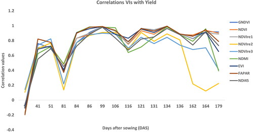
The nine VIs (NDVI, NDVIre1, NDVIre2, NDVIre3, NDI45, NDMI, GNDVI, FAPAR, and EVI) generated from Sentinel-2 data were tested for their correlation with the actual sunflower crop yield and predictive ability. The crop ages in the satellite images were calculated according to days after sowing (DAS). The correlation between the crop yield and VIs was calculated throughout the growing period, as shown in Figure 4. Then, the DAS at which each VI had the highest correlation to the crop yield was determined. The correlation between the VIs and crop yield was very low in the vegetative emergence and early reproductive stages (9–81 DAS). The correlation increased during the flowering stage (81–95 DAS) and peaked when the crops reached physiological maturity (98–116 DAS). This trend was reflected by the correlation coefficient (R-value), which was less than 0.2 at 10 DAS and reached a maximum of 0.68 at 99 DAS for EVI and FAPAR. Based on these results and considering the availability of satellite imagery, three dates were selected for model training: June 25, July 8, and July 13 corresponding to 86, 99, and 106 DAS.

Figure 4. Pearson correlation coefficient (r-value) between vegetation indices and observed crop yield during the sunflower growing season.

3.2. Remote sensing-based monitoring

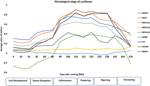
The RS-based monitoring of the sunflower growing period obtained a distinct temporal pattern, as shown in Figure 5. The crop phenology and transition dates were collected by measuring the VIs at random points in the 10 fields using the polygon tool in QGIS 3.16. Then, the randomly selected points were averaged and distributed throughout the sunflower development stages. The VIs based on plant spectral reflectance (NDVI, NDVIre1, NDVIre2, NDVIre3, NDI45, GNDVI, FAPAR, and EVI) had almost identical and consistent temporal patterns during the growing season. In contrast, NDMI showed a negative correlation with the water stress. The VIs were lowest during the initial stages of the growing season. After 40 DAS (around mid-May), NDMI increased in response to an increase in precipitation. After several weeks (9–86 DAS), the VIs rose steadily, which represented the start of the vegetative stages (i.e. seedling emergence and true leaf development) and rapid growth of the sunflowers. The growth of the sunflowers peaked at 86–116 DAS, which corresponded to the highest values for the VIs. The VIs decreased at 131–162 DAS, which indicated that the sunflowers had reached maturity and senescence. The VIs dropped to their lowest values at 162–179 DAS, which corresponded to the harvest time and was when the leaves dried and died.

Figure 5. Sunflower phenological stages based on Sentinel-2 VIs during the growing season.

3.3. Crop yield prediction

The effectiveness of the ML approaches at crop yield prediction was evaluated. We investigated the potential of the nine VIs at predicting the crop yield at the pixel level before harvesting. The VIs obtained on June 25, July 8, and July 13 at 86, 99, and 106 DAS were used because they showed the highest correlation with the actual crop yield (Figure 4).

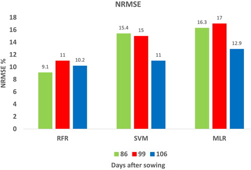
The results showed that the VIs could successfully predict the crop yield in the inflorescence emergence stage (86–116 DAS), which is when the vegetative growth of the sunflowers peaked. All three ML approaches showed the highest prediction accuracy at 99 DAS (July 8). RFR outperformed SVM and MLR. RFR realized the highest R² = 0.75, lowest RMSE of 0.361 kg\ha and NRMSE% of 11 on July 8 (Figures 6–8). Thus, the RFR model was applied to five independent sunflower fields for further validation.

Figure 6. Coefficient of determination (R²) for training fields with RFR, SVM, and MLR.

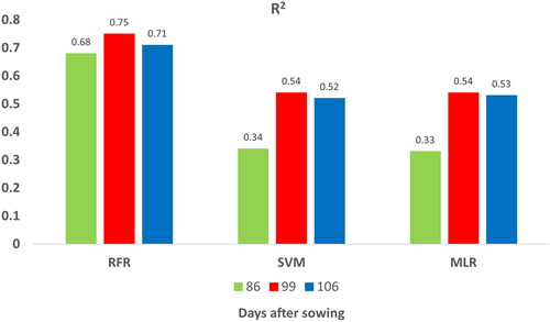
Figure 7. RMSE values for training fields with RFR, SVM, and MLR.

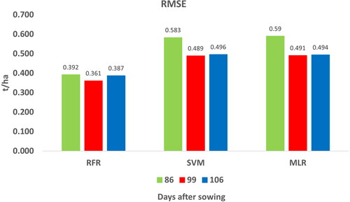
Figure 8. NRMSE% values for training fields with RFR, SVM, and MLR.

Further, the correlation matrix revealed a high correlation between NDI45 and NDVI (0.90), NDVIre1 and EVI (0.93), NDMI and FAPAR (0.92), GNDVI and FAPAR (0.90), and EVI and NDVIre1 (0.93) might indicate multicollinearity (Figure 9). The result of VIF and Tolerance shows the variables NDVI, NDVIre1, NDI45, and FAPAR have a Tolerance < 0.1 and a VIF above 40 (Table 4). Therefore, multicollinearity is highly likely. We excluded highly correlated Vis and run the MLR model again. However, prediction accuracy was noticeably decreased. Thus, we used all existing variables for further analysis.

Figure 9. The image above shows the correlation matrix of the variables that are included in our regression model.

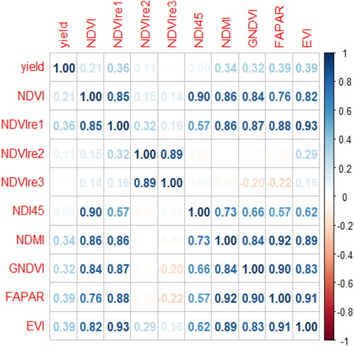
Table 4. Tolerance and VIFs values to detect multicollinearity.

Variables	Tolerance	VIF
NDVI	0.009495596	105.31198
NDVIre1	0.015239420	65.61930
NDVIre2	0.077675173	12.87413
NDVIre3	0.049541067	20.18527
NDI45	0.020329168	49.19040
NDMI	0.046560545	21.47741
GNDVI	0.078636104	12.71681
FAPAR	0.015980318	62.57698
EVI	0.030782124	32.48639

Note: Highly correlated variables are highlighted in red colour.

In order to evaluate the robustness of the RFR approach, different fields were combined to develop a suitable RFR model. To ensure the equal spatial distribution of the yield in the training dataset, Field 2 alone (89.9 ha), Fields 2 and 3 (112.5 ha), and Fields 4 and 5 according to the area of the fields were merged. The RFR models were run for each dataset. A combination of the different fields yielded significantly higher prediction accuracy (i.e. RMSE = 0.155 t/ha and R² = 0.89) in contrast with the earlier obtained best training RFR model (i.e. RMSE = 0.361 t/ha and R² = 0.75), respectively. Developed a new RFR model prediction that was evaluated in both pixel and field scales. For the pixel-level prediction, we created fishnet grid polygons with 60x30m dimensions that contain 18 Sentinel-2 pixels (Figure 10). Average VIs and crop yield values were calculated for corresponding grids. The pixel-based model showed an accurate prediction relative to the field scale prediction (Table 5)

Figure 10. Example of field boundary for pixel-level prediction.

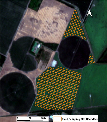
Table 5. Result of the pixel-level wheat yield estimation with RFR.

Parcel ID	R^2	RMSE	Parcel ID	R^2	RMSE
1	0.60	0.210	10	0.58	0.360
2	0.52	0.151	11	0.93	0.094
3	0.98	0.082	12	0.98	0.087
4	0.99	0.097	13	0.80	0.294
5	0.70	0.118	14	0.98	0.127
6	0.84	0.366	15	0.98	0.047
7	0.93	0.105	16	0.90	0.340
8	0.86	0.115	17	0.99	0.161
9	0.59	0.215	18	0.99	0.027

3.4. Spatial variability and validation

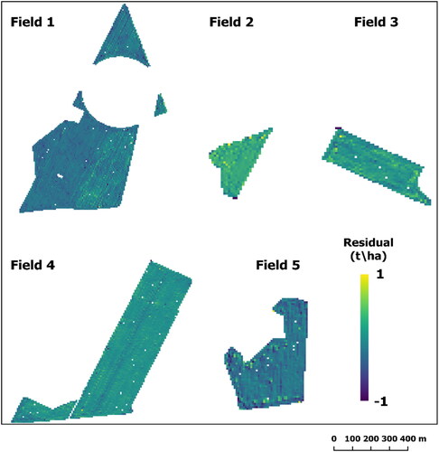
Actual spatial distribution of the crop yield within the field variability was created based on combine harvester data (Figure 11). Owing to RFR performing the best, this model was used to generate distribution maps of the predicted crop yield of the different fields. The predicted crop yield was correlated with the vegetation values. The predicted crop yields reflected the general pattern of the observed crop yields with relatively small variations within a specific field. For further comparison, residual maps were created by subtracting the predicted from the observed yield map, as shown in Figure 12. The map of residual yields also highlighted some areas underestimated and overestimated by the model. For Fields 1 and 5 the model slightly underestimated the crop yield for almost one-third of the area. For Fields 2, 3 and 4 the models accurately estimated the field-scale variability with few errors.

Figure 11. Observed crop yields of the test fields at the pixel level.

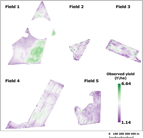
Figure 12. Residual maps. Differences between observed and predicted sunflower crop yield.

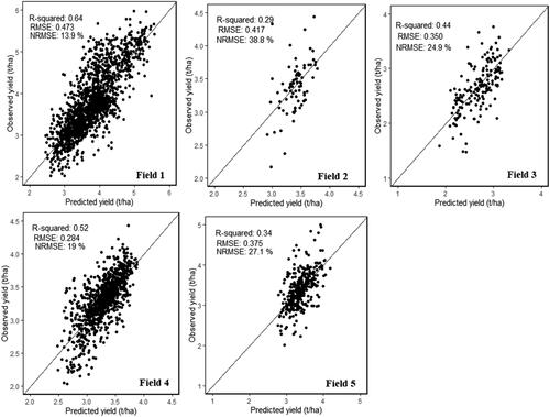
Regression analysis was performed between the observed and predicted crop yields for model validation (Figure 13). The scatter plots show a significant relationship between observed and predicted crop yields. The highest prediction accuracy was obtained for Field 4 with an RMSE of 0.284 t/ha. The model accuracy differed among fields, which had RMSE values ranging from 0.284 and 0.473 t/ha.

Figure 13. Scatter plots comparing the observed and predicted yields of the test fields.

4. Discussion

In this study, all VIs showed the highest correlation with the predicted crop yield at the inflorescence emergence stage. This is in line with the results of (Narin and Abdikan 2022), who also obtained the highest correlation in this stage. The highest correlation and lowest RMSE between the observed yield and VIs were obtained at June 25, July 8, and July 13 with all of the considered ML techniques. The most appropriate period for predicting and monitoring the crop yield was 86–116 DAS. RFR was shown to be the best ML approach for predicting the field-scale variability of the crop yield, with an R² value of almost 0.6 and RMSE of 0.284–0.473 t/ha. Several other studies have shown that RFR is an optimal ML technique for monitoring and predicting crop yields at the field or regional scale because of its high accuracy and precision (Jeong et al. 2016; Kayad et al. 2019; Amankulova et al. 2023).

The results showed that VIs could be used to accurately predict the crop yield in the middle and late growth stages according to the land surface phenology (LSP). It was not a possible direct geographical link between ground-observed phenology and S2-derived LSP. Because ground phenology was recorded by visual observation. However, we found that this temporal window has a strong correlation with temperature. The RS-derived VIs showed the highest correlation with the sunflower growth stage on the BBCH scale. Sentinel-2 satellites provide a 5-day temporal resolution under the cloud-free condition with a combined constellation, which allowed us to collect spectral reflectance data for each growth stage. Sentinel-2 images could serve as an important source of data for monitoring and predicting crop yields at the field scale to prevent economic losses.

Applying ML increased the prediction accuracy than using VIs alone, as demonstrated by the higher R² and lower RMSE. In particular, RFR performed well when trained at 99 DAS on a few ground truth samples and then applied to other test fields. This indicates that the training and test fields had similar characteristics. Mapping the spatial distribution of the crop yield over a field of interest could support farmers for site-specific applications.

The accuracy of the measured data affected the accuracy of the prediction model. The observed crop yield data provided by the combine harvester were used as the ground truth, but such equipment is prone to a degree of error. Incorrect data may be recorded for various reasons, such as signal delay, incorrect or inaccurate combine header status on some points, multiple combines in the same field calibrated differently, border effects, and GPS and sensor inaccuracies (Thylén and Murphy 1996; Blackmore and Marshall 2015). The relationship between the crop yield and VIs is affected by many factors including the soil type, nutrient content, topography, and farming practices ; it can be used to identify management zones, assess field-scale variability, and highlight the need for precision agriculture (PA) practices.

Our results showed that the reflectance of the sunflower plants increased from June to early August and decreased from late August until harvest time. According to the BBCH scale, early July is the flowering stage of sunflowers, which corresponded to the highest correlation for the VIs (Figure 4). Among the ML methods used to predict the crop yield, SVM and MLR performed similarly with RMSE values of 489 and 491.7, respectively, and R² values of 0.54 for both. RFR was very effective at crop yield prediction and outperformed MLR and SVM.

5. Conclusion

In this study, we evaluated the possibility of using RS-based imaging data to monitor and predict sunflower crop yields of 10 fields. We developed prediction models using VIs derived from Sentinel-2 MSI data to predict the crop yield before the harvest stage. Based on the correlation coefficient between the observed crop yield and VIs, we determined the best crop age for predicting the yield and the best ML approach for regression analysis:

• Among the VIs, EVI and FAPAR showed the highest correlation with the crop yield.

• The most appropriate time for using the VIs to predict the crop yield was during the peak vegetation period corresponding to the inflorescence emergence stage at 86–116 DAS.

• This period not only showed the highest correlation with the observed yield but also had relatively high satellite image availability because of the low number of cloud events during this time.

• Among the ML approaches, RFR performed the best at monitoring the field-scale variability of the crop yield with R² values of almost 0.6.

The results suggest that Sentinel-2 MSI products can be used to support monitoring, mapping, and predicting crop yields of small-scale and fragmented farmland, which will be helpful for agricultural decision-making and early warnings. Besides, we believe that the developed model can be applied to other crops and regions in Europe, especially Central European countries. Because Hungary has similar climatic conditions and crop types with relevance to European agricultural systems. Future research will focus on combining environmental variables (i.e. Topographic and soil moisture) derived from multisource satellite imagery with deep learning approaches for crop yield prediction. In addition, crop biophysical and biochemical parameters retrievable with radiative transfer models such as canopy nitrogen content, canopy chlorophyll content and canopy water content from spaceborne Hyperspectral imagery will be incorporated into the prediction model.

Acknowledgements

The authors want to thank ESA for the availability of Sentinel-2 MSI at Copernicus Open Access Hub. Sunflower yield data and phenological stages were collected at small-scale farmlands in collaboration with local farmers. We also would like to thank R software developers for such powerful program.

Data availability statement

All datasets R code used in this research are available from corresponding author upon reasonable request.

Disclosure statement

The authors have no conflicts of interest.

Additional information

Funding

This work was supported by the [University of Szeged Open Access Fund] under Grant [number 6076]; [Ministry of Innovation and Technology of Hungary through the National Research, Development and Innovation Fund Project TKP2021-NVA-09] under Grant.

Appendix 1.

Sentinel-2 bands that were used in this study

Table

Bands	Central Wavelength (nm)	Spatial Resolution (m)
Band 2 - Blue	490 nm	10 m
Band 3 - Green	560 nm	10 m
Band 4 - Red	665 nm	10 m
Band 5 - Vegetation red edge	705 nm	20 m
Band 6 - Vegetation red edge	740 nm	20 m
Band 7 - Vegetation red edge	783 nm	20 m
Band 8 - NIR	842 nm	10 m
Band 8A - Narrow NIR	865 nm	20 m
Band 11 - SWIR	1610 nm	20 m
Band 12 - SWIR	2190 nm	20 m

References

- Adeleke BS, Babalola OO. 2020. Oilseed crop sunflower (Helianthus annuus) as a source of food: nutritional and health benefits. Food Sci Nutr. 8(9):4666–4684.
- Amankulova K, Farmonov N, Gudmann A, Mucsi L. 2021. Investigation the reason of affected Hybrid Corn in Agricultural Fields by Using Multi-Temporal Sentinel-2 Images in Mezőhegyes, South-Eastern Hungary.
- Amankulova K, Farmonov N, Mucsi L. 2023. Time-series analysis of Sentinel-2 satellite images for sunflower yield estimation. Smart Agric Technol. 3:100098. https://doi.org/10.1016/j.atech.2022.100098.
- Andrianasolo FN, Casadebaig P, Maza E, Champolivier L, Maury P, Debaeke P. 2014. Prediction of sunflower grain oil concentration as a function of variety, crop management and environment using statistical models. Eur J Agron. 54:84–96.
- Bell MA. 1994. Guide to plant and crops sampling: measurements and observations for agronomic and physiological research in small grain cereals. Mexico: CIMMYT.
- Blackmore BS, Marshall CJ. 2015. Yield mapping; errors and algorithms. In: robert PC, Rust RH, Larson WE., editors, ASA, CSSA, and SSSA Books. Madison, WI, USA: American Society of Agronomy, Crop Science Society of America, Soil Science Society of America; p. 403–415.
- Breiman L. 2001. Random forests. ]Mach Learn. 45(1):5–32.
- Bolton DK, Friedl MA. 2013. Forecasting crop yield using remotely sensed vegetation indices and crop phenology metrics. Agric For Meteorol. 173:74–84.
- Chen X, Feng L, Yao R, Wu X, Sun J, Gong W. 2021. Prediction of maize yield at the city level in China using multi-source data. Remote Sens. 13(1):146.
- Das AC, Noguchi R, Ahamed T. 2021. An assessment of drought stress in tea estates using optical and thermal remote sensing. Remote Sens. 13(14):2730.
- European Space Agency. STEP—Science Toolbox Exploitation Platform. [accessed 2021 Feb 15] 362. http://step.esa.int.
- Fieuzal R, Marais Sicre C, Baup F. 2017. Estimation of sunflower yield using a simplified agrometeorological model controlled by optical and SAR satellite data. IEEE J Sel Top Appl Earth Observ Remote Sens. 10(12):5412–5422.
- Ghosh P, Mandal D, Bhattacharya A, Nanda MK, Bera S. 2018. Assessing crop monitoring potential of sentinel-2 in a spatio-temporal scale. Int Arch Photogramm Remote Sens Spatial Inf Sci. XLII–5:227–231. https://doi.org/10.5194/isprsarchives-XLII-5-227-2018
- Gitelson AA, Kaufman YJ, Merzlyak MN. 1996. Use of a green channel in remote sensing of global vegetation from EOS-MODIS. Remote Sens Environ. 58(3):289–298.
- Guo Y, Fu Y, Hao F, Zhang X, Wu W, Jin X, Robin Bryant C, Senthilnath J. 2021. Integrated phenology and climate in rice yields prediction using machine learning methods. Ecol Indic. 120:106935.
- Haerani H, Apan A, Basnet B. 2018. Mapping of peanut crops in Queensland, Australia, using time-series PROBA-V 100-m normalized difference vegetation index imagery. J Appl Remote Sens. 12(03):1.
- Huang J, Wang X, Li X, Tian H, Pan Z. 2013. Remotely sensed rice yield prediction using multi-temporal NDVI data derived from NOAA’s-AVHRR. PLoS ONE. 8(8):e70816.
- Huete A, Didan K, Miura T, Rodriguez EP, Gao X, Ferreira LG. 2002. Overview of the radiometric and biophysical performance of the MODIS vegetation indices. Remote Sens Environ. 83(1-2):195–213.
- Huete AR. 1988. A soil-adjusted vegetation index (SAVI). Remote Sens Environ. 25(3):295–309.
- Hunt ML, Blackburn GA, Carrasco L, Redhead JW, Rowland CS. 2019. High resolution wheat yield mapping using Sentinel-2. Remote Sens Environ. 233:111410.
- Jaafar HH, Ahmad FA. 2015. Crop yield prediction from remotely sensed vegetation indices and primary productivity in arid and semi-arid lands. Int J Remote Sens. 36(18):4570–4589.
- Jeong JH, Resop JP, Mueller ND, Fleisher DH, Yun K, Butler EE, Timlin DJ, Shim K-M, Gerber JS, Reddy VR, et al. 2016. Random forests for global and regional crop yield predictions. Plos One. 11(6):e0156571.
- Jin X, Kumar L, Li Z, Xu X, Yang G, Wang J. 2016. Estimation of winter wheat biomass and yield by combining the AquaCrop model and field hyperspectral data. Remote Sens. 8(12):972.
- Kayad A, Sozzi M, Gatto S, Marinello F, Pirotti F. 2019. Monitoring within-field variability of corn yield using sentinel-2 and machine learning techniques. Remote Sens. 11(23):2873.
- Kayad AG, Al-Gaadi KA, Tola E, Madugundu R, Zeyada AM, Kalaitzidis C. 2016. Assessing the spatial variability of alfalfa yield using satellite imagery and ground-based data. Plos One. 11(6):e0157166.
- Khaki S, Wang L. 2019. Crop yield prediction using deep neural networks. Front Plant Sci. 10:621.
- Kharel TP, Maresma A, Czymmek KJ, Oware EK, Ketterings QM. 2019. Combining spatial and temporal corn silage yield variability for management zone development. Agron J. 111(6):2703–2711.
- Kim N, Lee Y-W. 2016. Machine learning approaches to corn yield estimation using satellite images and climate data: a case of Iowa State. J. Korean Soc. Surv. Geod. Photogramm. Cartogr. 34(4):383–390.
- Li W, Weiss M, Waldner F, Defourny P, Demarez V, Morin D, Hagolle O, Baret F. 2015. A Generic algorithm to estimate LAI, FAPAR and FCOVER variables from SPOT4_HRVIR and landsat sensors: evaluation of the consistency and comparison with ground measurements. Remote Sens. 7(11):15494–15516.
- Liaw A, Wiener M, Breimann L, Cutler A. 2018. Randomforest: breiman and Cutler’s random forests for classification and regression. [accessed 2021 Jan 15]. https://cran.r-project.org/web/packages/randomForest/randomForest.pdf
- Lancashire PD, Bleiholder H, Boom TVD, Langelüddeke P, Stauss R, Weber E, Witzenberger A. 1991. A uniform decimal code for growth stages of crops and weeds. Ann Appl Biol. 119(3):561–601.
- Lokupitiya E, Denning S, Paustian K, Baker I, Schaefer K, Verma S, Meyers T, Bernacchi CJ, Suyker A, Fischer M. 2009. Incorporation of crop phenology in Simple Biosphere Model (SiBcrop) to improve land-atmosphere carbon exchanges from croplands. Biogeosciences. 6(6):969–986.
- Micheneau A, Champolivier L, Dejoux J-F, Ahmad AB, Pontet C, et al. 2017. Predicting sunflower grain yield using remote sensing data and statistical models. 2017 EFITA WCCA Congress, Jul 2017, Montpellier, France. 254 p. ffhal-02737612f.
- Mitchell JJ, Glenn NF, Sankey TT, Derryberry DR, Germino MJ. 2012. Remote sensing of sagebrush canopy nitrogen. Remote Sens Environ. 124:217–223.
- Narin OG, Abdikan S. 2022. Monitoring of phenological stage and yield estimation of sunflower plant using Sentinel-2 satellite images. Geocarto Int. 37(5):1378–1392.
- Narin OG, Sekertekin A, Saygin A, Balik Sanli F, Gullu M. 2021. Yield estimation of sunflower plant with CNN and ANN using sentinel-2. Int Arch Photogramm Remote Sens Spatial Inf Sci. XLVI-4/W5-2021:385–389.
- OECD, Food and Agriculture Organization of the United Nations. 2016. OECD-FAO Agricultural Outlook 2016-2025, OECD-FAO Agricultural Outlook. OECD.
- Operational drought and water scarcity management system (OVF). [accessed 2022 Feb 15]. https://aszalymonitoring.vizugy.hu/
- Open Access Hub. [accessed 2021 Sep 1]. https://scihub.copernicus.eu/..
- Pal US, Patra RK, Sahoo NR, Bakhara CK, Panda MK. 2015. Effect of refining on quality and composition of sunflower oil. J Food Sci Technol. 52(7):4613–4618.
- Panda SS, Ames DP, Panigrahi S. 2010. Application of vegetation indices for agricultural crop yield prediction using neural network techniques. Remote Sens. 2(3):673–696.
- Panek E, Gozdowski D. 2020. Analysis of relationship between cereal yield and NDVI for selected regions of Central Europe based on MODIS satellite data. Remote Sens Appl Soc Environ. 17:100286.
- Piragnolo M, Masiero A, Pirotti F. 2017. Open source R for applying machine learning to RPAS remote sensing images. Open Geospatial Data Softw Stand. 2:16.
- Pirotti F, Sunar F, Piragnolo M. 2016. Benchmark of machine learning methods for classification of a sentinel-2 image. Int Arch Photogramm Remote Sens Spatial Inf Sci. XLI-B7:335–340.
- Ruml M, Vulic T. 2005. Importance of phenological observations and predictions in agriculture. J Agric Sci BGD. 50(2):217–225.
- Satir O, Berberoglu S. 2016. Crop yield prediction under soil salinity using satellite derived vegetation indices. Field Crops Res. 192:134–143.
- Schwalbert RA, Amado T, Corassa G, Pott LP, Prasad PVV, Ciampitti IA. 2020. Satellite-based soybean yield forecast: integrating machine learning and weather data for improving crop yield prediction in southern Brazil. Agric For Meteorol. 284:107886.
- Shammi SA, Meng Q. 2021. Use time series NDVI and EVI to develop dynamic crop growth metrics for yield modeling. Ecol Indic. 121:107124.
- Singh R, Semwal DP, Rai A, Chhikara RS. 2002. Small area estimation of crop yield using remote sensing satellite data. Int J Remote Sens. 23(1):49–56.
- Sakamoto T, Gitelson AA, Arkebauer TJ. 2013. MODIS-based corn grain yield estimation model incorporating crop phenology information. Remote Sens Environ. 131:215–231.
- Szabó S, Szopos NM, Bertalan-Balázs B, László E, Milošević DD, Conoscenti C, Lázár I. 2019. Geospatial analysis of drought tendencies in the carpathians as reflected in a 50-year time series. HunGeoBull; 68(3):269–282.
- Thylén L, Murphy DPL. 1996. The control of errors in momentary yield data from combine harvesters. J Agric Eng Res. 64(4):271–278.
- Trépos R, Champolivier L, Dejoux J-F, Al Bitar A, Casadebaig P, Debaeke P. 2020. Forecasting sunflower grain yield by assimilating leaf area index into a crop model. Remote Sens. 12(22):3816.
- Tucker CJ. 1979. Red and photographic infrared linear combinations for monitoring vegetation. Remote Sens Environ. 8(2):127–150.
- Wang AX, Tran C, Desai N, Lobell D, Ermon S. 2018. Deep Transfer Learning for Crop Yield Prediction with Remote Sensing Data. In Proceedings of the 1st ACM SIGCAS Conference on Computing and Sustainable Societies. ACM, Menlo Park, Netherlands and San Jose CA USA; p. 1–5.
- Wang M, Tao F, Shi W. 2014. Corn yield forecasting in Northeast China using remotely sensed spectral indices and crop phenology metrics. J Integr Agric. 13(7):1538–1545.
- Xue J, Su B. 2017. Significant remote sensing vegetation indices: a review of developments and applications. J Sens. 2017:1–17.
- Zhou J, Khot LR, Bahlol HY, Boydston R, Miklas PN. 2016. Evaluation of ground, proximal and aerial remote sensing technologies for crop stress monitoring. IFAC-Pap. 49:22–26.