Modelling of land use and land cover changes and prediction using CA-Markov and Random Forest

Abstract

We used the Cellular Automata Markov (CA-Markov) integrated technique to study land use and land cover (LULC) changes in the Cholistan and Thal deserts in Punjab, Pakistan. We plotted the distribution of the LULC throughout the desert terrain for the years 1990, 2006 and 2022. The Random Forest methodology was utilized to classify the data obtained from Landsat 5 (TM), Landsat 7 (ETM+) and Landsat 8 (OLI/TIRS), as well as ancillary data. The LULC maps generated using this method have an overall accuracy of more than 87%. CA-Markov was utilized to forecast changes in land usage in 2022, and changes were projected for 2038 by extending the patterns seen in 2022. A CA-Markov-Chain was developed for simulating long-term landscape changes at 16-year time steps from 2022 to 2038. Analysis of urban sprawl was carried out by using the Random Forest (RF). Through the CA-Markov Chain analysis, we can expect that high density and low-density residential areas will grow from 8.12 to 12.26 km² and from 18.10 to 28.45 km² in 2022 and 2038, as inferred from the changes occurred from 1990 to 2022. The LULC projected for 2038 showed that there would be increased urbanization of the terrain, with probable development in the croplands westward and northward, as well as growth in residential centers. The findings can potentially assist management operations geared towards the conservation of wildlife and the eco-system in the region. This study can also be a reference for other studies that try to project changes in arid are as undergoing land-use changes comparable to those in this study.

Keywords:

• CA-Markov
• LULC
• change detection
• simulation
• Thal and Cholistan

1. Introduction

Alterations to land use and land cover (LULC) are widely recognized as one of the most significant environmental concerns on a worldwide scale (Syed et al. 2014; Hussain et al. 2022b; Islam et al. 2022). Major contributors to biodiversity decline include variations in LULC, the concomitant loss of habitat and habitat fragmentation (Becker et al. 2013; Bera et al. 2022; Khalil et al. 2022). Human actions (such as subsequent land degradation, urbanization, deforestation, overgrazing and agricultural intensification) are typically blamed for these changes; however, natural forces can also play a role in their development (Xie et al. 2013; Fu et al. 2022). The transition to intensive agriculture and excessive grazing are two of the primary factors contributing to the deterioration of land in dry regions. These changes, which humans cause, can lead to a depletion of natural resources and impact the sustenance stock in these regions, which can have simple repercussions for society and politics (Liu and Hwang 2015; Haq et al. 2022).

In order to assess the viability of standardizing and integrating data sets and making maps, it is essential to make accurate predictions about how land will be used. There are many benefits to using a logistic regression model instead of a conventional one (combined with other models but do not clarify the relative importance of the motivating factors). The CA-Markov model is a cross between CA (an exposed formation that can be easily linked with knowledge-driven models) and the Markov Chain model (accurate spatial and temporal modeling) (Mansour et al. 2022). In order to construct the Markov chain, we make use of a collection of probability values that, on the basis of past data, reflect the likelihood of future alterations to user interfaces. It is possible that land use classifications to change in any given location of the world at any given moment (Hussain et al. 2020). CA-Markov can be used to assess the probability of transition for a variety of land use interactions across time. One or more types of land use may come to predominate in a region as a result of these scale changes. Matrixes depicting the area’s transformation across time are generated by counting the number of pixels that belong to various land use classes at various epochs. Coating kinds have found use, as mentioned in a Markov chain (Mansour et al. 2020).

After performing an analysis on the land use zoning images using the Markov chain model, the model generates an output image as well as a possible change matrix that is based on the potential change matrix from the previous year (Tariq and Qin 2023). A change matrix depicts the potential for transitions in land use in the future. When simulating the effects of changes in land use, the bottom-up markov chain and cellular automata model is a useful tool. As an approachable geographical model for LULC forecasting based on the identification of the dynamics of complex systems. Moreover, it is acknowledged as a valid two-dimensional approach to depicting the spatial and temporal dynamics of position (Zhang et al. 2019). Markov models work well in both temperate and hot environments, as well as at a range of sizes (Jalayer et al. 2022; Esmaeili et al. 2023).

The CA-Markov model was proposed in this research as a means of simulating real-world scenarios; it mixes Cellular Automata and Markov Chains. The probabilities of changes between different types of land cover over a particular period of time are typically determined using a Markov chain model. These probabilities are then used in a CA model to generate spatially explicit forecasts that change over time. Assuming that the drivers that cause the observed patterns of land cover categories will continue to act in the future as they have in the past, the initial distribution and transition matrix form the basis of a CA-Markov model (Jones et al. 2012; Tariq et al. 2022a). When taking a counterfactual approach, a CA-Markov model is useful because it permits us to project forward the state of the landscape prior to intervention under the assumption that the intervention type will be maintained (Fensholt and Sandholt 2005; Baqa et al. 2022). The ability to predict LULC change has been used in urban planning by modelling rural development and urban growth. Arshad et al.(2008) identifying high-priority conservation zones, and determining appropriate conservation responses (Tariq et al. 2022a, 2022b); reviewing the diminuendos of variation farming (Arshad et al. 2008) and simulating rangeland subtleties underneath a variety of climate change situations.

Adopting Markov chain models presents a hurdle due to the assumption of stationary transitions, which is one of the reasons why it is more suited for short-term predictions than long-term projections (Tariq et al. 2022c). Furthermore, the Markov chain analysis, by itself, is not considered to be spatially explicit (Rehman et al. 2017; Khan et al. 2022). This is because the analysis does not offer a geographical dispersal of the verification, which is essential in comprehending the possible influence of predicted variations. This limitation of the method can be remedied by integrating it with various other dynamic and empirical models. Felegari (2021) explained that integrated modelling techniques are the best way to show how land-use changes over time in the most accurate way.

There are several different sizes at which these models have been applied to predict and simulate changes in land usage (Arshad et al. 2008; Tariq and Shu, 2020; Tariq et al. 2020). As a spatial transition model, the CA-Markov technique in this study merges stochastic spatial Markov methods with the stochastic spatial CA method (Arshad et al. 2008). There are two-way transitions between LULC classes, unlike the Geomod method, which only predicts loss or gain in one direction between classes. This is an advantage since it allows for more accurate forecasting (Tariq et al. 2022a). They discovered that regression-based models fared substantially worse than transition-based models, which integrate the spatial Markov model with the spatial CA-Markov model. The study identified six major LULC classes most suitable for predicting the distribution of LULC using the CA-Markov-Chain. The main goals of this research were (1) identification and monitoring of LULC in the area between 1990, 2006 and 2022, and (2) using the CA-Markov method on these LULC maps to predict possible deviations in the year 2022 and 2038.

2. Study area

The Cholistan Desert, also called Rohi in its native language in Pakistan, is located approximately 30 km to the west of Bahawalpur in the province of Punjab. It extends over an area of more than 26,000 km² and makes up the southern portion of what was formerly the Bahawalpur division of southern Punjab. It takes up approximately 2/3rd of the land that used to be the Bahawalpur division. This desert has an approximate length of 480 km and a width ranging from 27°42′00ʺ to 29°45′00ʺ N and 69°57′30ʺ to 72°52′30ʺ E (Baloch et al. 2021; Moazzam et al. 2022) (Figure 1). The Thal desert is located between two rivers in the province of Punjab on Sind Sagar Doab. Its coordinates are 31°10′ N and 71°30′ E. It is a huge region located south of the Pothohar Plateau and between the Jhelum and Indus rivers. It has a length of around 300 km from north to south and a width of approximately 110 km from east to west (Imran et al. 2022) (Figure 1). The average annual precipitation in this region is 100–150 mm, giving it a dry environment. It is characterized by two geomorphologic components (Tariq et al. 2021b). The northern sector of plain is characterized by a group of elongated calcareous ridges that originated in the ocean not too long ago (Zamani et al. 2022).

Figure 1. (a) Country-based location of the study area; (b) map of the study area; (c) geographical location of the study area in Pakistan.

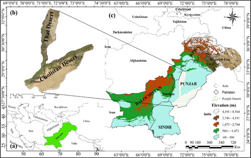
Approximately 83% of the dunes in deserts have been developed into resorts and hotels for tourists. In addition, the installation of an irrigation network resulted in the fragmentation of the habitat of a non-saline depression, which led to a drop in the size of the habitat by around 35%. Since 2001, no investigations have been carried out in either the Thal or Cholistan regions simultaneously.

3. Material and methods

3.1. Remote sensing with ancillary data

Satellites images of the Landsat (TM) 5, (ETM+) 7 and (OLI) 8 were obtained on three separate periods to investigate how the terrain has evolved over the past three decades, explained in the Table 1. We converted the Landsat Digital Numbers (DN), also known as DNs, to spectral brightness measured in absolute units at the sensor. Alternatively, TOA reflectance values can be estimated from DN by using these two steps: Compute the radiance values ($L_{\lambda }$), from the DN. ${\mathrm{Gain}}_{\lambda }$ and ${\mathrm{Bais}}_{\lambda }$ are the gain and offset values for each spectral band ($\lambda$), respectively (Shah et al. 2022).

Table 1. Landsat data were used in this research.

Satellite	Sensor	Acquisition date	Path	Row	Source
Landsat 4–5	TM	May 8, 1990	178	39	https://earthexplorer.usgs.gov/
Landsat 7	ETM+	May 11, 2006	178	39
Landsat 8	OLI/TIRS	May 17, 2022	178	39

Based on level II of the LULC categorization system developed by Anderson et al. (1976), this study region is divided into six different LULC categories (Table 2). The research location has a limited plant cover and a highly reflective background, which suggests that there may be difficulties in identifying LULC classes based only on spectral data. It has been discovered that the accuracy of LULC classification may be improved by using methods that integrate auxiliary data with spectral data (Tariq et al. 2021a).

Table 2. LULC classifications mapped in the area across the three research periods are described below (Anderson et al. 1995).

LULC classes	Code	LULC classes	Current study code	Description
Residential	11	High-density residential area	HDR	Areas populated by small towns, villages and outlying industrial sites and roadways
Residential	11	Low-density residential area	LDR	You’ll find small towns, villages, industrial regions and major roads in the countryside
Cropland	21	Cropland	CR	Irrigated areas and used primarily for the production of crops
Water	5	Water	W	Areas covered by water/wetlands. Halophytic plants grow in saline soil in wet regions
Barren area	74	Barren area	BA	Barren land with less vegetation
Gravel desert	75	Gravel desert	GD	No vegetation or minimal vegetation in areas covered by stones, gravel and coarse sand

SRTM 30 m grid spacing DEM version 4.1 was included in the supplemental information (Ghaderizadeh et al. 2021). The terrain roughness index, aspects and length of the slope were all included in the parameters. System for Automated Geoscientific Analyses (SAGA-GIS v_2.0.7) was used to determine the land surface values of LULC (Tariq and Shu 2020). It was also included because of the southwest locational pattern of the LULC classes identified in the area during field studies. The addition of texture to the classification process helped to improve the results. The GLCM (Grey Level Co-occurrence Matrix) was constructed using a kernel of $3\mathrm{ }\times 3$ pixels from the Near Infra-red (NIR) band. Also included were the tasselled cap’s greenness, brightness and wetness spectral indices (Tariq and Shu 2020).

3.2. Random Forest classification

Random Forest (RF) classification was utilized in the experiment. This method can give a more accurate classification than current methods (Ok et al. 2012; Pelletier et al. 2016; Aslam et al. 2021). Because of this, it’s been proven more resistant to outliers and noise (Ullah et al. 2017). Many different decision trees make up the tree-based ensemble classifier known as RF (Isuhuaylas et al. 2018). We randomly choose subsets of the original training data set for ensemble tree training and then replace them with new ones. The DTs in the ensemble are randomly partitioned into subsets using a random subset of k predictors. Every model in the ensemble will be unique because of these random processes. After running many tree models, the ensemble’s final categorization is decided by a simple majority of the DTs. RF models consisting of 300 trees were used to categorize the remote sensing data collected during each of the three distinct time periods. Many DTs and variable number combinations at the split nodes were tested before settling. The RF package (Khan et al. 2020) was used in R software to perform the classification.

3.2.1. Training data and accuracy assessment

The Landsat images indicates the precision and terrain corrected data which provides systematic geometric and radiometric accuracy by incorporating ground control points (GCPs). We also used the digital topographic map of 1:150,000 scale and the Global Positing System (GPS). A field survey conducted between March and June 2022 obtained 30 representative GPS points per class except water class. Generally, residential areas, cropland, water bodies, road intersections and barren land areas were identified as major GCPs and these references are located near the corners and the middle of the study area. Using stratified random sampling, ground reference data were gathered. There were $30\mathrm{ }\times 30$m designs for each of the plots. Each plot was given a LULC class identification number based on the data collected in the field. About 70% of the reference data was used to train the classifier, and the other 30% was used to test the accuracy assessment. The vector map layers were generated using various vector and grid data formats, such as population settlements and density, highways, railways and DEM (30 m) which was used to generate slopes, aspects and elevation. In this analysis, LULC classification was implemented based on six classes and a brief description of major LULC classes is provided in Table 2. Classification accuracy procedures were developed using confusion matrices, including commission and omission errors, overall accuracy and kappa value. These classification accuracy matrices were derived using confusion matrices (Mumtaz et al. 2020; Tariq and Shu, 2020). The commission error, as measured against independent data sources, is the fraction of pixels that were improperly classified. On the other hand, the percentage of pixels that should have been assigned to a particular class according to the reference data but have not been assigned to that class is an omission error. It was figured out how to determine the omission and commission error for individually LULC and estimate the typical for all classes (see Supplementary Table 1).

3.3. Prediction of LULC change

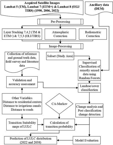
CA-Markov is a reliable method for predicting changes in LULC, and it has been advocated as the method of choice since it outperforms other methods (Potapov et al. 2012). In addition, it can forecast transitions between LULC classes in both directions (Pourghasemi et al. 2013). The use of a CA-Markov model resulted in three steps of prediction for the upcoming change in LULC: (1) calculating transition matrices from LULC maps from 1990, 2006 and 2022; (2) calculating the LULC transition potential maps and (3) using the CA model to anticipate the geographical distribution of LULC by applying it to the variations matrices as well as the potential transition maps.

3.3.1. Transition probabilities

The Markov model was used to make projections about the dispersal of LULC class (shown in Figure 2), with the projections being based on the transition probability p_ij between any two LULC classes ($i$ and $j$). Over the period of t seconds to t seconds plus one, the following formula was used to calculate p_ij in Equation (1); (1) $$\mathit{pij}=\frac{\mathit{nij}}{nj}$$(1)

Figure 2. Diagrammatic representation of the research approach taken for this investigation.

The dispersal of each LULC class was predictable using the Markov model (Figure 2), and the projections were based on the transition probability $\mathrm{pij}$ between each pair of LULC classes ($i$ and $j$). p_ij was calculated as the following during a certain period beginning at time $t$ and ending at time $tp1$ in eq. 2; (2) $${\sum }_{j=1}^k\mathit{pij}=1$$(2) where n_i = total number of pixels from each class $i$ that have been changed during the transition time, n_ij is the number of pixels that have been transformed from class $i$ to class $j,$ and $k$ is the total number of LULC classes were calculated in in Equation (3); (3) $$p\mathrm{*}Mt=Mt+1$$(3)

LULC dispersal at the starting time $t (Mt$) and the transition probability matrix $p$ were used to project forward the dispersal of each LULC class at time $t+1\mathrm{ }(Mt+1$).

The LULC maps for the years 1990, 2006 and 2022 that were the result of the classification procedure were utilized in calculating utilizing a first-order Markov model between the periods of 1990 and 2006, 2006 and 2022 and 1990 and 2022 (Moazzam et al. 2022; Tariq et al. 2022a). After that, these transition matrices were used in the many processes that comprised the prediction of LULC change.

3.3.2. Transition suitability maps

The appropriateness of each pixel, as defined by suitability maps, can be transitioned to any of the LULC classes. A number from 0 to 255 is assigned to each pixel that makes up the suitability maps. A value of 0 indicates an area not appropriate for a certain LULC class, while a value of 255 indicates that the area is extremely suitable for that class. Between 1990 and 2022, key transitions between LULC classes were utilized to create transition rules and restrictions for each LULC class to produce transition suitability maps. Field surveys determined these transitions, previous studies (Tariq et al. 2021b, 2023), and the writers’ prior understanding of the subject matter. There were a variety of factors, and they all changed throughout time (e.g. distance to the nearest road, number of population centers nearby and the location of an irrigation canal system). There is a good chance that the presence of an existing LULC class will also impact the destiny of this new class. The distance to the nearest road, the number of population centers nearby and the location of an irrigation canal system were some considerations that went into developing the LULC transition potential maps.

As an illustration, water, ridges and uncultivated land all acted as barriers to the transition to agricultural practices. In the constraints layers, locations with a value of 1 are evaluated as f appropriateness, while places with a value of 0 are evaluated as unsuited for a particular LULC (Boolean constraints). The weighted linear combination approach and the Boolean logical operations were used to create transition suitability maps. Weighted factors (distance to the nearest road, the number of population centers nearby and the location of an irrigation canal system) and Boolean restrictions are criteria utilized the linear mixture method during the development of suitability maps. When using logic and operations, finding the connection of criteria will lead to finding the appropriate extents for a certain LULC class. The next step was to use the transition suitability maps to estimate how the LULC will be spread out in 2022 and to simulate how it will be spread out in 2038.

3.3.3. Markov chain-cellular automata model

When modelling LULC in 2022, we used a mixed CA-Markov technique. The transition probabilities covered 1990–2006; we used the LULC base map from 2006 as our starting point. Based on the transition probabilities, an estimation was made of the amount of area that would need to be transferred from one LULC class to another. A contiguity filter was used to assign weights to the various suitability factors. The suitability of pixels located a significant distance away from the pixel that was going to be converted was given less weight. The neighbourhood rules were defined with the help of a contiguity filter with a size of $5\times 5\mathrm{ }$ pixels. Each pixel will be put into a LULC class based on how well it fits that class and how close it is to other pixels in the each class.

The simulation will proceed until the area of each LULC that has to be converted during each iteration (determined by the transition probability matrix) has been reached. The kappa statistic was utilized to evaluate the unity between the projected LULC map for 2022 and the actual LULC map for 2022, hence determining the accuracy of the predicted map. Pontius and Millones’ method was used to calculate the degree to which the two maps’ spatial patterns were compatible with one another, and from there, agreement and disagreement components were calculated to use in a model validity assessment (2022). The CA-Markov method was then used to forecast the LULC in the study area to the year 2038, following the same procedures. To do this, we made use of the LULC base map for 2022 and the simulated results for the years 2006–2022. IDRISI Selva was used as a background for this investigation (Palsson et al. 2017).

4. Results

4.1. Land use and land cover changes

Applying RF to categorize the TM satellite imageries for the years 1990, ETM + satellite images in 2006 and OLI satellite images for the years 2022 resulted in the production of LULC maps (Figure 3) with OA of more than 86% and KIA ≥ 0.8 (Table 3). However, omission and commission mistakes differed from class to class within LULC (Figure 4). There were higher rates of commission and omission mistakes (10–27%), particularly for heterogeneous classes like HDR, LDR and OA, because they were often misidentified. The OA class is an example of a diverse group because it includes both orchards and farms that rely on rainfed circumstances. In this part of the world, orchards are often comprised of relatively modest spaces that are annexed to the homes of the locals and surrounded by walls made of limestone bricks. Therefore, some of these regions can be confused with the HDR and LDR classes (Hussain et al. 2022a; Wahla et al. 2022).

Figure 3. Classification of Landsat TM, ETM + and OLI images in three stages: (a) 1990, (b) 2006 and (c) 2022.

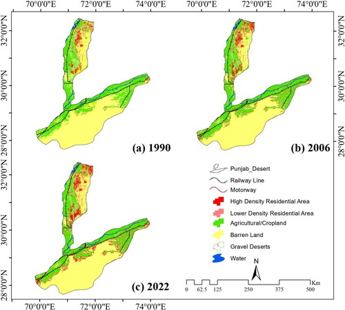
Figure 4. The percentage of errors due to omission and commission error for each LULC class on the categorized maps in the years 1990, 2006 and 2022, respectively.

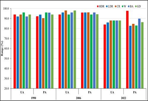
Table 3. The overall accuracy, the KIA, the mean error per class and the commission error for the LULC categorization for the years 1990, 2006 and 2022 are all presented here.

Years (stage)	OA	Kappa	Mean omission/class (%)	Mean commission/class (%)
1990	93.67	0.82	6.96 ± 7.46	7.90 ± 8.62
2006	90.33	0.82	5.98 ± 4.07	5.09 ± 6.46
2022	87.00	0.81	2.75 ± 4.13	3.02 ± 3.51

The inland plateau is the Barren Area (BA) with a low vegetative area (5%) class on all three classification maps. This class predominates in the study area’s middle latitudes (Figures 3 and 5). Cropland (CR) is one of this area’s most significant land uses. The Gravel Desert (GD) class, which is representative of the gravelly plain, encompasses most of the southern portion of the terrain (about 30%). The northern half of the area covers the remaining LULC classes, and the majority of these classes may be found in the northern half of the area.

Figure 5. During 1990, 2006, 2022 and 2038, the total area of LULC classes was expressed as a proportion of the total area of the landscape.

More information, including trends and rates of land-use change, can be gleaned from the LULC maps. The findings provide light on the land-use change history as well as the magnitude of land-use change in each LULC category. The land passed through three distinct stages, with each map depicting a different period. These stages were distinguished from one another by the kinds of land use activities that predominated in each stage (Figures 3 and 5). During the first stage of development in the region, which the map from 1990 depicts, the primary land use was grazing, followed by agriculture (Hu et al. 2021; Felegari et al. 2022; Moazzam et al. 2022). Barren land, also known as BA, covered more than 34% of the land area. Orchards and rain-fed agriculture comprised much less of the agricultural activities carried out during this period (around 2.45%). At this point, very few croplands were irrigated. This was partly due to the absence of water sources sustaining extensive irrigated agriculture (Mumtaz et al. 2021; Sharifi et al. 2022; Zamani et al. 2022). High-density residential areas (HDR) and Less Residential Areas (LDR) combined occupied only about 1% of the study area. HDR areas include residential areas, roadways and other types of built-up regions. Water areas are also included in this category (Figures 3 and 5). Before, they lived off of things like grazing, farming that depended on the rain, gathering medicinal plants and sometimes working as guards in quarries (Yang et al. 2018).

Some variations in the dispersal of each LULC were found in the second stage, which is reflected by the 2006 LULC map. The lands under CR control were cut in half due to the development of an extensive irrigation canal network and seasonal tourist attractions (Figure 3). The irrigation canal network was considered part of the HDR and LDR class even though, at this point, the network was still being constructed, and not all of its branches had water in them. For the purpose of reclaiming arid land for agricultural use, the government funded the construction of this irrigation system. During this time period, water was only permitted to be released into a single canal system branch in the northeastern corner of the study region. Consequently, activity related to irrigated agriculture started to extend across the northeastern part of the region. Consequently, the amount previously devoted to agriculture dependent on rainfall decreased. BA also rose during this period due to the availability of water, which was something (Ma et al. 2019; Tariq and Mumtaz, 2022; Majeed et al. 2023; Tariq et al. 2023). As water is usually regarded a restriction for all LULC classes in the research area, this work used three constraints: distance to the nearest road, the number of population centers nearby and the position of the irrigation canals.

These patterns in built up area and agricultural pursuits are visible in the third stage of the process (2022 map). Built-up areas have grown by around 180% since 1990, Rural Expansion areas (RE) grew by 140% and farmland areas grew by 170%. Because there was no water in any of the irrigation canals branches during the second stage, there was a restriction placed on the amount of land that could be farmed. In the third stage, releasing water into more canal branches increased the rate of gain in farmland areas (Figure 6). This expansion of cropland areas occurred westward between the years 2006 and 2022.

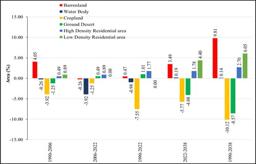
Figure 6. Rate of gain/loss (km²/year) for each LULC class during various periods.

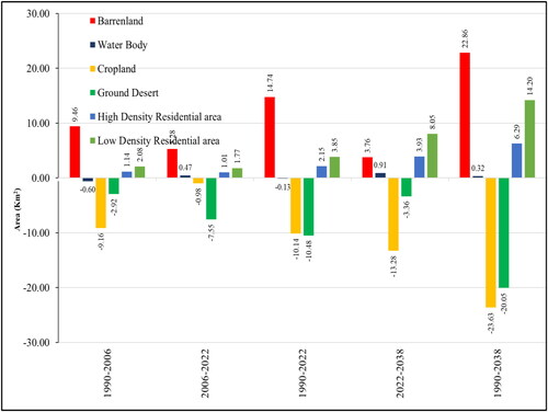
The pattern of change displayed by some of the LULC remained consistent; these LULC have either accrued gains or suffered losses at varying rates depending on the period (Figure 6). This was different for both the orchards and other cropland activities (CR) class as well as the HDR and LDR class. For instance, HDR and LDR all demonstrated growth throughout the whole study period, albeit at varying rates from one period to the next (Figure 6). However, compared to the period from 1990 to 2006, the rates of gain in LDR and HDR, and W have slowed down from 2006 to 2022 (Tariq et al. 2022c).

In contrast, CR and HDR growth rates accelerated between 2006 and 2022. The discrepancy in these land uses’ rates of return could be attributed to socioeconomic considerations. The slowdown in the pace of gain in real estate between 2006 and 2022 was because, by 2022, most of the water and parts of the cropland had been converted into resorts. Because the few tiny patches of CR still around today fall under the purview of GD, they are being safeguarded and preserved to serve as a model for the habitat type that may be found in the surrounding region. According to the results of a study by Tariq and Shu (2020) between 1990 and 2006 that looked at how fragmented the habitat was in GD, about 83% of the coastal dunes were close to HDR, and LDR had been turned into resorts, and tourist villages.

Compared to the period between 1990 and 2006, the rate of gain in Barren land (BA) was significantly higher than 2006–2022. In the time period 2006–2022, the majority of quarrying activity was focussed on the inland area (Figure 3). The majority of the quarrying activities that were taking place in the northern region of the study have been put on hold since huge portions of the calcareous ridges in that region have been levelled down and devoured as a result of these activities (Mousa et al. 2020). Between 1990 and 2006, several quarrying operations were carried out inside the boundaries of OBR. After the Pakistan Meteorological Department (PMD) and the Urban Unit, this practice stopped (Mumtaz et al. 2021). Therefore, this event is connected to the temporal dynamics of the many land uses that make use of these various natural land covers.

There was a reduction in LDR between 1990 and 2006, but a rise between 2006 and 2022. Over the course of the study period, which began in 1990 and ended in 2022, salt marshes and other wet areas lost almost 36% of their original area. This may be because some water (W) has been converted into built-up areas and roads. However, between 2006 and 2022, approximately 91% of this land cover’s transformed area was converted into built-up areas, resorts, croplands and orchards. After being drained, the coastal marshes and other wet regions were allowed to dry out before being converted into tourist destinations. After abandoning the locals built new settlements and planted orchards in the wetlands to the south of the dunes. At the close of the 1990s (Majeed et al. 2021) and the beginning of the second stage picked up speed and became more pronounced. Residents of the area have gained access to an increased number of employment prospects as a direct result of the quickening pace at which summer resorts are being built along the center. This has led to a boom in the tourist and recreation industries in the region. Jobs created at hotels and quarries, as well as greater commerce in land parcels, helped raise the standard of living in the surrounding areas. Since then, many have moved out of tents and into newly built homes, and their fig and fruit orchard yields have skyrocketed.

4.2. LULC changes and prediction

Using the transition trend, as shown by Markov transition matrices covering the years 1990–2022, we can identify three distinct eras in the landscape’s evolution (Table 4). The possibility that a particular type of land cover would persist from $t = 0 \mathrm{to} t = 1$ is represented by the diagonal values of each transition matrix. The values signify the probabilities that one type of LC will changes into alternative. For example, GD, W and BA all have transition probabilities that are greater than 0.75 and have the highest probability of remaining unchanged throughout the entire period from 1990 to 2022. This gives them the highest probability of remaining unchanged. Other CR and LDR quarries had the lowest probabilities of the species persisting in their environments. During the period between 2006 and 2022, the LULC classifications that were the most consistent were W, GD and BA. It was more likely that once the farmland areas were constructed, they would be used for producing crops regularly, especially because the irrigation system was established as part of the government. Therefore, once the cropland areas were established, they were used for growing crops. The reason that the CR class persisted was that the area was designated for touristic facilities. This was done as part of a goal to promote the area by simultaneously bolstering agricultural and tourism-related endeavours. Other classes like HDR, LDR areas and quarries were the LULC classes that had the lowest transition persistence, but they were also the ones that had the most active LULC classes overall.

Table 4. A Markov chain matrix represents the probability of LULC transitions from 1990–2006 and 2006–2022.

From	LULC	Period	To
			HDR	LDR	CR	W	BA	GD
	HDR	1990–2006	0.63	0.04	0.05	0.04	0.01	0.01
		2006–2022	0.07	0.03	0.04	0.02	0.03	0.03
	LDR	1990–2006	0.03	0.03	0.04	0.04	0.04	0.01
		2006–2022	0.05	0.07	0.03	0.03	0.03	0.04
	CR	1990–2006	0.03	0.01	0.02	0.02	0.01	0.03
		2006–2022	0.02	0.03	0.01	0.03	0.05	0.02
	W	1990–2006	0.07	0.03	0.03	0.05	0.08	0.02
		2006–2022	0.03	0.03	0.05	0.06	0.03	0.01
	BA	1990–2006	0.05	0.01	0.03	0.02	0.02	0.01
		2006–2022	0.04	0.05	0.04	0.01	0.02	0.02
	GD	1990–2006	0.04	0.07	0.03	0.01	0.03	0.01
		2006–2022	0.03	0.03	0.02	0.00	0.02	0.02

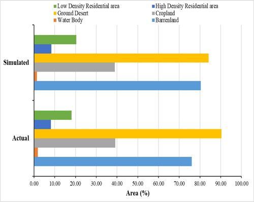
When the 2022 LULC map was compared to the map predicted using the CA Markov approach (Table 5), it was found that there was both maps accord rather well with one another. Both maps had an OA of more than 80%, and their kappa was greater than 0.80. There were a total of six classes. All five achieved a PA and UA of more than 85% (Table 5). The highest levels of KIA were achieved by HDR and BA, both of which had OA values greater than 0.86.

Table 5. Comparing 2022 LULC predictions with 2022 LULC measurements.

	HDR	LDR	CR	W	BA	GD
PA	92.00	84.62	87.76	86.79	91.49	88.00
UA	90.20	88.00	86.00	92.00	86.00	88.00
K	0.81
OA	86.71
Mean omission/class		7.23 ± 8.23
Mean commission/class		9.05 ± 6.25

On the other hand, 2022 map, CR, W, BA and GD have higher value of UA and HDR, and LDR, achieved the lowest levels of agreement, each of which had UA values of 84%, and 86%, respectively. Figure 7 showed that LULC change was created correctly with an agreed amount of 19.8% and that it was placed in the proper allocation with an agreed location of 62.5%. There is a difference in amount and location, but the overall disparity (total disagreements) is less than 10%. According to the findings, the CA Markov model was successful in making a prediction of the LULC for the year 2022. What this means is that the system can be used to foretell future land use changes in the region, provided that the rate of change are expected to remain constant.

Figure 7. A contrast between the observed LULC and the actual LULC in 2022.

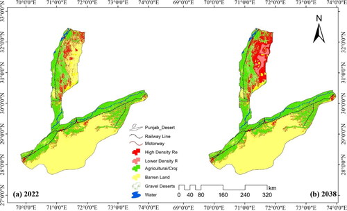
The projection of the possible distribution of LULC classes in 2038, shown in Figure 3(d), shows an extension of croplands to the west and the north. In addition, it demonstrates a rise in the number of regional quarries and residential centers and a growth in the number of resorts in the area located on the dunes.

4.3. Model validation

The following steps were taken using IDRISI and Image Processing software’s help to implement the CA-Markov model in the research setting: Maps of prospective land use transitions are generated using a process, transition probabilities are calculated using Markov chain analysis, and simulated land use probabilities are distributed using a CA spatial filter. By using the present-day distributions of the Thal and Cholistan deserts as a starting state, a CA-Markov model was able to project future changes in land use patterns in the year 2038 with a confidence interval of 16 years. Not only can the Markov transition matrix provide a quantitative explanation for the changes in land use, it may also disclose the rate at which these changes occur. The Table 6 conversion matrices of land use types from 1990–2022 can be summed up as follows:

Table 6. Transition probabilities matrix of land use types in Thal and Cholistan deserts during 1990–2022 (units in %).

LULC classes	Code	HDR	LDR	CR	W	BA	GD
Residential	HDR	87.21	0.28	4.07	0	7.96	0.48
Residential	LDR	1.72	90.43	1.61	0.41	5.26	0.57
Cropland	CR	0.44	0.51	97.53	0	1.29	0.23
Water	W	4.58	1.24	0.45	89.82	3.43	0.21
Barren area	BA	0.44	0.26	0.62	0	98.01	0.07
Gravel desert	GD	0.15	0.07	0.18	3.20	0.15	96.25

5. Discussion

The changes in land cover that are taking place in the region reflect the policy adopted by the government of Pakistan, which is to expand outside of the valley and by developing desert fringe areas. Tourism and agricultural reclamation initiatives were to be the focus of the development plan for the desert in the region’s northern corner. According to the current study’s findings, the most significant factors that led to changes in the area were most likely the construction of a summer resort near the urban area and the installation of an irrigation system (Halmy et al. 2015).

The natural land cover would likely deteriorate due to the existing tendency of changing LULC due to built up area. Therefore, the pressure placed on these places will continue to increase, and it is anticipated that areas such as rangelands, salt marshes, near highways and human settlements will become prime candidates for transformation (Felegari et al. 2021). So, it’s possible that species’ ecological niches will be constrained and eventually disappear due to habitat fragmentation and size reduction.

The results of the area change shown in Figure 8 indicate that the area of urbanized regions will expand by 2038. In the next few years, we expect an increase of around 12.26 km² in the developed regions. As seen in Figure 9, the findings of the spatial distribution show that all land-cover classes will show concentrated spatial distribution patterns, with urban built-up land expanding to suburban areas and vegetation in the suburbs quickly converting into built-up land.

Figure 8. Area change of land-cover classes from 2022 to 2038.

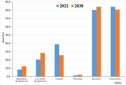
Figure 9. Simulated map of land-cover type from 2022 to 2038.

According to Baqa et al. (2022), the formation of summer resorts caused damage to vegetation of the coastal dunes, which in turn led to the loss of several of the indigenous species that had previously inhabited this region. Understanding how land use changes may affect natural landscapes is possible via the use of maps developed by this research project. As a reference for conservation planning in the area, our simulation results might aid decision-makers in refining land use management plans to strike a balance between development and conservation (Kamusoko et al. 2009; Radwan et al. 2019). The pressure on the remaining rangeland regions may need to be reduced in plans, and the westward cropland extension may need to be stopped. To reduce the degree to which the coastal and inland ridges are broken up, increased regulation of the quarrying operations might be an option. There may be a need to restrict the growth of summer resorts on coastal dunes to preserve the small number of coastal dunes included in the research region.

In this work, the CA-Markov model was utilized to predict the evolution of LULC changes between 2022 and 2038 (Aburas et al. 2017). Using multisource data with auxiliary data, six commonly used land cover intelligent classification techniques were used to determine the condition of LULC in Thal and Cholistan. Cellular automata and Markov chain analysis are two mathematical models used to study complex systems such as urban growth and land use change. Cellular automata models are based on a grid of cells that can have different states, and the states of these cells change over time according to a set of rules. Markov chain analysis, on the other hand, is a statistical method that models the probability of transitioning from one state to another in a system with a finite number of states.

While both models have their strengths, they also have limitations when applied to complex systems. One limitation of cellular automata models is that they are often based on simple rules that may not accurately capture the complexity of real-world systems. For example, they may not account for the influence of social, economic and political factors on land use change. In addition, cellular automata models are often sensitive to the initial conditions, meaning that small changes in the starting conditions can lead to significant differences in the final outcomes.

Markov chain analysis, on the other hand, assumes that the future state of a system depends only on the current state and not on the history of the system. This assumption may not hold in complex systems where the future state may depend on past events and conditions. In addition, Markov chain models may not account for the interactions between different variables in the system, which can limit their ability to accurately predict the behaviour of the system.

In conclusion, while cellular automata and Markov chain analysis are valuable tools for studying complex systems, they have limitations that must be taken into account when applying them to real-world problems. It is important to use a combination of different models and data sources to gain a more comprehensive understanding of complex systems and make informed decisions.

6. Conclusion

In this study, we used Landsat TM, ETM + and OLI imagery were used for mapping of LULC distributions for the years 1990, 2006 and 2022 integrated with environmental variables. The RF technique successfully classified the LULC in a portion of Pakistan’s Thal and Cholistan desert regions. The RF technique successfully classified the LULC in a portion of Pakistan’s Thal and Cholistan desert regions using Landsat imagery integrated with environmental variables,. To model the long-term evolution of the terrain from 2022 to 2038, a CA-Markov-Chain was built with 16-year time increments. This indicates that this method can reliably map LULC in similar arid and semi-arid eco-systems. Over the past three decades, LULC in the region have undergone three distinct stages of transition as a direct result of the development activities that have been carried out in the area. At each stage, a distinctive pattern of land use predominated. Quarrying, grazing and non-irrigated agriculture were the primary economic activities of the first stage (rain-fed and orchards). Increased summer resorts and built-up regions marked the second stage, as did the demand that went along with it, leading to a rise in quarrying. This time period saw the expansion of both rain-fed and irrigated (orchard) farming as well as the development of the region’s irrigation network. When the irrigation network started to work in the third stage of development, orchards and other forms of farming that depended on rain fell out of favour. At the same time, the number of built-up areas and resorts grew.

Both the CA model and the Markov Chain analysis were used to make predictions regarding the temporal resolution of the data. The CA model was utilized to identify changes in the spatial distribution of the organisms. Researchers and policymakers will use this model to design new regulations to control and manage metropolitan areas’ growth.

Author contributions

Muhammad Asif: conceptualization, methodology, software, formal analysis, visualization, data curation, writing—original draft, investigation, validation, writing—review and editing; Jamil Hasan Kazmi: writing—review and editing; Aqil Tariq: methodology, software, formal analysis, visualization, data curation, writing—original draft, investigation, validation, writing—review and editing, Supervision, Na Zhao: methodology, software, formal analysis, visualization, data curation, writing—original draft, investigation, validation, writing—review and editing, Funding. Rufat Guluzade: writing—review and editing. Walid Soufan: writing—review and editing. Khalid F. Almutairi: writing—review and editing. Ayman El Sabagh: writing—review and editing. Muhammad Aslam: writing—review and editing. All authors have read and agreed to the published version of the manuscript.

Acknowledgements

This is part of the PhD research work of the first author. We are thankful to all the reviewers and editor to modify this paper during the review process. This research was funded by the Re-searchers Supporting Project No. (RSP D2023R561), King Saud University, Riyadh, Saudi Arabia.

Disclosure statement

No potential conflict of interest was reported by the authors. Moreover, the writers have thoroughly addressed ethical issues, including plagiarism, informed consent, fraud, data manufacturing and/or falsification, dual publication and/or submission and redundancy.

Data availability statement

The data presented in this study are available on request from the first or corresponding authors.

Additional information

Funding

Major Program of National Natural Science Foundation of China (No. 42293270), the Na-tional Program of National Natural Science Foundation of China (No. 42071374). This research was funded by the Researchers Supporting Project No. (RSPD2023R561), King Saud University, Riyadh, Saudi Arabia.

References

- Aburas MM, Ho YM, Ramli MF, Ash’aari ZH. 2017. Improving the capability of an integrated CA-Markov model to simulate spatio-temporal urban growth trends using an Analytical Hierarchy Process and Frequency Ratio. Int J Appl Earth Obs Geoinf. 59:65–78.
- Anderson CA, Deuser WE, DeNeve KM. 1995. Hot temperatures, hostile affect, hostile cognition, and arousal: tests of a general model of affective aggression. Pers Soc Psychol Bull. 21(5):434–448.
- Anderson JR, Hardy EE, Roach JT, Witmer RE. 1976. A land use and land cover classification system for use with remote sensor data. Professional Paper.
- Arshad M, Yasin Ashraf M, Noureen S, Moazzam M. 2008. Edaphic factors and distribution of vegetation in the Cholistan Desert, Pakistan. Pak J Bot. 40:1923–1931.
- Aslam B, Zafar A, Khalil U. 2021. Development of integrated deep learning and machine learning algorithm for the assessment of landslide hazard potential. Soft Comput. 25(21):13493–13512.
- Baloch MYJ, Zhang W, Chai J, Li S, Alqurashi M, Rehman G, Tariq A, Talpur SA, Iqbal J, Munir M, et al. 2021. Shallow groundwater quality assessment and its suitability analysis for drinking and irrigation purposes. Water (Switzerland). 13(23):3361.
- Baqa MF, Lu L, Chen F, Nawaz-Ul-Huda S, Pan L, Tariq A, Qureshi S, Li B, Li Q. 2022. Characterizing spatiotemporal variations in the urban thermal environment related to land cover changes in Karachi, Pakistan, from 2000 to 2020. Remote Sens. 14(9):2164.
- Becker A, Finger P, Meyer-Christoffer A, Rudolf B, Schamm K, Schneider U, Ziese M. 2013. A description of the global land-surface precipitation data products of the Global Precipitation Climatology Centre with sample applications including centennial (trend) analysis from 1901-present. Earth Syst Sci Data. 5(1):71–99.
- Bera D, Das Chatterjee N, Mumtaz F, Dinda S, Ghosh S, Zhao N, Bera S, Tariq A. 2022. Integrated influencing mechanism of potential drivers on seasonal variability of LST in Kolkata Municipal Corporation, India. Land. 11(9):1461.
- Esmaeili M, Abbasi-Moghadam D, Sharifi A, Tariq A, Li Q. 2023. Hyperspectral image band selection based on CNN embedded GA (CNNeGA). IEEE J Sel Top Appl Earth Obs Remote Sens. 1–27.
- Felegari S, Sharifi A, Moravej K. 2022. Investigation of the relationship between NDVI Inde, soil moisture, and precipitation data using satellite images. Sustainability. 11(21):12.
- Felegari S, Sharifi A, Moravej K, Amin M, Golchin A, Muzirafuti A, Tariq A, Zhao N. 2021. Integration of Sentinel 1 and Sentinel 2 Satellite images for crop mapping. Appl Sci. 11(21):10104.
- Fensholt R, Sandholt I. 2005. Evaluation of MODIS and NOAA AVHRR vegetation indices with in situ measurements in a semi-arid environment. Int J Remote Sens. 26(12):2561–2594.
- Fu C, Cheng L, Qin S, Tariq A, Liu P, Zou K, Chang L. 2022. Timely plastic-mulched cropland extraction method from complex mixed surfaces in arid regions. Remote Sens. 14(16):4051.
- Ghaderizadeh S, Abbasi-Moghadam D, Sharifi A, Zhao N, Tariq A. 2021. Hyperspectral image classification using a hybrid 3D-2D convolutional neural networks. IEEE J Sel Top Appl Earth Obs Remote Sens. 14:7570–7588.
- Halmy MWA, Gessler PE, Hicke JA, Salem BB. 2015. Land use/land cover change detection and prediction in the north-western coastal desert of Egypt using Markov-CA. Appl Geogr. 63:101–112.
- Haq SM, Tariq A, Li Q, Yaqoob U, Majeed M, Hassan M, Fatima S, Kumar M, Bussmann RW, Moazzam M, et al. 2022. Influence of edaphic properties in determining forest community patterns of the Zabarwan Mountain Range in the Kashmir Himalayas. Forests. 13(8):1214.
- Hu P, Sharifi A, Tahir MN, Tariq A, Zhang L, Mumtaz F, Shah, SHI, A. 2021. Evaluation of vegetation indices and phenological metrics using time-series modis data for monitoring vegetation change in Punjab, Pakistan. Water (Switzerland). 13(18):2550.
- Hussain S, Lu L, Mubeen M, Nasim W, Karuppannan S, Fahad S, Tariq A, Mousa BG, Mumtaz F, Aslam M. 2022a. Spatiotemporal variation in land use land cover in the response to local climate change using multispectral remote sensing data. Land. 11(5):595.
- Hussain S, Mubeen M, Akram W, Ahmad A, Habib-Ur-Rahman M, Ghaffar A, Amin A, Awais M, Farid HU, Farooq A, et al. 2020. Study of land cover/land use changes using RS and GIS: a case study of Multan district, Pakistan. Environ Monit Assess. 192(1):2.
- Hussain S, Qin S, Nasim W, Bukhari MA, Mubeen M, Fahad S, Raza A, Abdo HG, Tariq A, Mousa BG, et al. 2022b. Monitoring the dynamic changes in vegetation cover using spatio-temporal remote sensing data from 1984 to 2020. Atmosphere (Basel). 13(10):1609.
- Imran M, Ahmad S, Sattar A, Tariq A. 2022. Mapping sequences and mineral deposits in poorly exposed lithologies of inaccessible regions in Azad Jammu and Kashmir using SVM with ASTER satellite data. Arab J Geosci. 15(6):538.
- Islam F, Riaz S, Ghaffar B, Tariq A, Shah SU, Nawaz M, Hussain ML, Amin NU, Li Q, Lu L, et al. 2022. Landslide susceptibility mapping (LSM) of Swat District, Hindu Kush Himalayan region of Pakistan, using GIS-based bivariate modeling. Front Environ Sci. 10:1–18.
- Isuhuaylas L, AV, Hirata Y, Santos L, CV, Torobeo NS. 2018. Natural forest mapping in the Andes (Peru): a comparison of the performance of machine-learning algorithms. Remote Sens. 10(5):782.
- Jalayer S, Sharifi A, Abbasi-Moghadam D, Tariq A, Qin S. 2022. Modeling and predicting land use land cover spatiotemporal changes: a case study in Chalus Watershed, Iran. IEEE J Sel Top Appl Earth Obs Remote Sens. 15:5496–5513.
- Jones MO, Kimball JS, Jones LA, McDonald KC. 2012. Satellite passive microwave detection of North America start of season. Remote Sens. Environ. 123:324–333.
- Kamusoko C, Aniya M, Adi B, Manjoro M. 2009. Rural sustainability under threat in Zimbabwe – simulation of future land use/cover changes in the Bindura district based on the Markov-cellular automata model. Appl Geogr. 29(3):435–447.
- Khalil U, Azam U, Aslam B, Ullah I, Tariq A, Li Q, Lu L. 2022. Developing a spatiotemporal model to forecast land surface temperature: a way forward for better town planning. Sustainability. 14(19):11873.
- Khan AM, Li Q, Saqib Z, Khan N, Habib T, Khalid N, Majeed M, Tariq A. 2022. MaxEnt modelling and impact of climate change on habitat suitability variations of economically important Chilgoza Pine (Pinus gerardiana Wall.) in South Asia. Forests. 13(5):715.
- Khan N, Sachindra DA, Shahid S, Ahmed K, Shiru MS, Nawaz N. 2020. Prediction of droughts over Pakistan using machine learning algorithms. Adv Water Resour. 139:103562.
- Liu Y, Hwang Y. 2015. Improving drought predictability in Arkansas using the ensemble PDSI forecast technique. Stoch Environ Res Risk Assess. 29(1):79–91.
- Ma L, Liu Y, Zhang X, Ye Y, Yin G, Johnson BA. 2019. Deep learning in remote sensing applications: a meta-analysis and review. ISPRS J Photogramm Remote Sens. 152:166–177.
- Majeed M, Lu L, Anwar MM, Tariq A, Qin S, El-Hefnawy ME, El-Sharnouby M, Li Q, Alasmari A. 2023. Prediction of flash flood susceptibility using integrating analytic hierarchy process (AHP) and frequency ratio (FR) algorithms. Front Environ Sci. 10:1–14.
- Majeed M, Tariq A, Anwar MM, Khan AM, Arshad F, Mumtaz F, Farhan M, Zhang L, Zafar A, Aziz M, et al. 2021. Monitoring of land use—land cover change and potential causal factors of climate change in Jhelum district, Punjab, Pakistan, through GIS and multi-temporal satellite data. Land. 10(10):1026.
- Mansour S, Al-Belushi M, Al-Awadhi T. 2020. Monitoring land use and land cover changes in the mountainous cities of Oman using GIS and CA-Markov modelling techniques. Land Use Policy. 91:104414.
- Mansour S, Alahmadi M, Atkinson PM, Dewan A. 2022. Forecasting of built-up land expansion in a Desert Urban Environment. Remote Sens. 14(9):2037.
- Moazzam MFU, Rahman G, Munawar S, Tariq A, Safdar Q, Lee B. 2022. Trends of rainfall variability and drought monitoring using standardized precipitation index in a scarcely gauged basin of Northern Pakistan. Water. 14(7):1132.
- Mousa BG, Shu H, Freeshah M, Tariq A. 2020. A novel scheme for merging active and passive satellite soil moisture retrievals based on maximizing the signal to noise ratio. Remote Sens. 12(22):3804.
- Mumtaz F, Arshad A, Mirchi A, Tariq A, Dilawar A, Hussain S, Shi S, Noor R, Noor R, Daccache A, et al. 2021. Impacts of reduced deposition of atmospheric nitrogen on coastal marine eco-system during substantial shift in human activities in the twenty-first century. Geomat Nat Hazards Risk. 12(1):2023–2047.
- Mumtaz F, Tao Y, de Leeuw G, Zhao L, Fan C, Elnashar A, Bashir B, Wang G, Li L, Naeem S, et al. 2020. Modeling spatio-temporal land transformation and its associated impacts on land surface temperature (LST). Remote Sens. 12(18):2987.
- Ok AO, Akar O, Gungor O. 2012. Evaluation of random forest method for agricultural crop classification. Eur J Remote Sens. 45(1):421–432.
- Palsson F, Sveinsson JR, Ulfarsson MO. 2017. Multispectral and hyperspectral image fusion using a 3-D-convolutional neural network. IEEE Geosci Remote Sens Lett. 14(5):639–643.
- Pelletier C, Valero S, Inglada J, Champion N, Dedieu G. 2016. Assessing the robustness of Random Forests to map land cover with high resolution satellite image time series over large areas. Remote Sens Environ. 187:156–168.
- Potapov PV, Turubanova SA, Hansen MC, Adusei B, Broich M, Altstatt A, Mane L, JuSTice CO. 2012. Quantifying forest cover loss in Democratic Republic of the Congo, 2000–2010, with Landsat ETM + data. Remote Sens Environ. 122:106–116.
- Pourghasemi HR, Moradi HR, Fatemi Aghda SM. 2013. Landslide susceptibility mapping by binary logistic regression, analytical hierarchy process, and statistical index models and assessment of their performances. Nat Hazards. 69(1):749–779.
- Radwan TM, Blackburn GA, Whyatt JD, Atkinson PM. 2019. Dramatic loss of agricultural land due to urban expansion threatens food security in the Nile Delta, Egypt. Remote Sens. 11(3):332.
- Rehman A, Jingdong L, Chandio AA, Hussain I. 2017. Livestock production and population census in Pakistan: determining their relationship with agricultural GDP using econometric analysis. Inf. Process Agric. 4(2):168–177.
- Shah S, HIA, Jianguo Y, Jahangir Z, Tariq A, Aslam B. 2022. Integrated geophysical technique for groundwater salinity delineation, an approach to agriculture sustainability for Nankana Sahib Area, Pakistan. Geomatics Nat Hazards Risk. 13(1):1043–1064.
- Sharifi A, Mahdipour H, Moradi E, Tariq A. 2022. Agricultural field extraction with deep learning algorithm and satellite imagery. J Indian Soc Remote Sens. 50(2):417–423.
- Syed FS, Iqbal W, Syed AAB, Rasul G. 2014. Uncertainties in the regional climate models simulations of South-Asian summer monsoon and climate change. Clim Dyn. 42(7-8):2079–2097.
- Tariq A, Mumtaz F. 2022. Modeling spatio-temporal assessment of land use land cover of Lahore and its impact on land surface temperature using multi-spectral remote sensing data. Environ Sci Pollut Res. 30(9):23908–23924.
- Tariq A, Mumtaz F, Majeed M, Zeng X. 2023. Spatio-temporal assessment of land use land cover based on trajectories and cellular automata Markov modelling and its impact on land surface temperature of Lahore district Pakistan. Environ Monit Assess. 195(1):114.
- Tariq A, Mumtaz F, Zeng X, Baloch MYJ, Moazzam MFU. 2022a. Spatio-temporal variation of seasonal heat islands mapping of Pakistan during 2000–2019, using day-time and night-time land surface temperatures MODIS and meteorological stations data. Remote Sens Appl Soc Environ. 27:100779.
- Tariq A, Qin S. 2023. Spatio-temporal variation in surface water in Punjab, Pakistan from 1985 to 2020 using machine-learning methods with time-series remote sensing data and driving factors. Agric Water Manag. 280:108228.
- Tariq A, Riaz I, Ahmad Z, Yang B, Amin M, Kausar R, Andleeb S, Farooqi MA, Rafiq M., 2020. Land surface temperature relation with normalized satellite indices for the estimation of spatio-temporal trends in temperature among various land use land cover classes of an arid Potohar region using Landsat data. Environ Earth Sci. 79(1):15.
- Tariq A, Shu H. 2020. CA-Markov chain analysis of seasonal land surface temperature and land use landcover change using optical multi-temporal satellite data of Faisalabad, Pakistan. Remote Sens. 12(20):3402.
- Tariq A, Shu H, Gagnon AS, Li Q, Mumtaz F, Hysa A, Siddique MA, Munir I. 2021a. Assessing burned areas in wildfires and prescribed fires with spectral indices and SAR images in the Margalla Hills of Pakistan. Forests. 12(10):1371.
- Tariq A, Shu H, Siddiqui S, Imran M, Farhan M. 2021b. Monitoring land use and land cover changes using geospatial techniques, a case study Of Fateh Jang, Attock, Pakistan. GES. 14(1):41–52.
- Tariq A, Yan J, Gagnon AS, Riaz Khan M, Mumtaz F. 2022b. Mapping of cropland, cropping patterns and crop types by combining optical remote sensing images with decision tree classifier and random forest. Geo-Spatial Inf Sci. 1–19.
- Tariq A, Yan J, Mumtaz F. 2022c. Land change modeler and CA-Markov chain analysis for land use land cover change using satellite data of Peshawar, Pakistan. Phys. Chem Earth A/B/C. 128:103286.
- Ullah S, Shafique M, Farooq M, Zeeshan M, Dees M. 2017. Evaluating the impact of classification algorithms and spatial resolution on the accuracy of land cover mapping in a mountain environment in Pakistan. Arab J Geosci. 10(3).
- Wahla SS, Kazmi JH, Sharifi A, Shirazi SA, Tariq A, Joyell Smith H. 2022. Assessing spatio-temporal mapping and monitoring of climatic variability using SPEI and RF machine learning models. Geocarto Int. 37(27):14963–14982.
- Xie H, Ringler C, Zhu T, Waqas A. 2013. Droughts in Pakistan: a spatiotemporal variability analysis using the Standardized Precipitation Index. Water Int. 38(5):620–631.
- Yang J, Zhao YQ, Chan, JC, W. 2018. Hyperspectral and multispectral image fusion via deep two-branches convolutional neural network. Remote Sens. 10(5):800.
- Zamani A, Sharifi A, Felegari S, Tariq A, Zhao N. 2022. Agro climatic zoning of saffron culture in Miyaneh City by using WLC method and remote sensing data. Agriculture. 12(1):118.
- Zhang H, Ning X, Shao Z, Wang H. 2019. Spatiotemporal pattern analysis of China’s cities based on high-resolution imagery from 2000 to 2015. IJGI. 8(5):241.
- Zhang Z, Hu B, Jiang W, Qiu H. 2021. Identification and scenario prediction of degree of wetland damage in Guangxi based on the CA-Markov model. Ecol Indic. 127:107764.