Inversion of intertidal zone topography based on optimized random forest regression characteristic parameters

Abstract

It is a fundamental task to monitor the topography and understand the changes of intertidal zone for rational utilization and sustainable development. A new method is proposed for identifying the terrain of the intertidal zone, using ICESat-2 data to replace a large amount of on-site observation data, thereby reducing costs and improving efficiency. Based on pre-experiments and correlation analysis, time phase index, water index, water transparency index and suspended sediment concentration index are added as features for the random forest (RF). Compared with using only the original band as the model input, the RMSE is reduced by 0.08 m. The results show that the inverted terrain has an RMSE of 0.45 m compared with handheld RTK data, and the RMSE at the mudflat from UAV data is 0.20 m. Based on the analysis of terrain changes over the four-year period, the trend towards sedimentation closer to land becomes more pronounced.

Keywords:

• Intertidal zone
• topography inversion
• ICESat-2 Data
• time phase
• random forest
• mudflat

1. Introduction

The global intertidal zone between mean high and mean low tide is a wide area of transition zone between ocean and land, with vast mudflat resources (Gao 2009; Zhi et al. 2022). The large mudflats in the intertidal zone are the habitat of many animals on earth, such as shellfish, birds and molluscs (Luijendijk et al. 2018). Since the development of the intertidal zone has a high economic value for coastal cities (Costanza et al. 1997), it is one of the most exposed areas to natural (e.g. storm surges, seawater inundation, sea level rise, etc.) and human activities (Erlandson 2008). In 2011, the State Council proposed the ‘ecological red line’ policy, in which wetland red line was listed as an important policy. The intertidal zone, as an important wetland carrier and habitat, also requires protection (Lin et al. 2016). Accurately identifying the boundary between protection and development of the intertidal zone is crucial for its rational utilization and sustainable development. Monitoring intertidal topography and understanding intertidal change are therefore essential for sustainable coastal development (Bishop-Taylor et al. 2019; Dai et al. 2018). With the increase in the number and variety of satellites around the world, it has become easier to obtain timely and accurate information about the Earth. The use of satellite data to obtain intertidal target information is faster and more timely than traditional mapping methods, which is particularly important for rapidly analysing the characteristics of intertidal zone changes, exploring the process of intertidal zone transitions, and providing technical support for scientific research on coastal development and protection.

A combination of remote sensing and in situ observations is a flexible and effective way to obtain intertidal topography (Gao et al. 2021; Yang, Xiao, et al. 2021; Zhou et al. 2021). Many studies have already used LiDAR data (Andriolo et al. 2018; Miles et al. 2019), Synthetic Aperture Radar data (Heygster et al. 2010; Zhang, Xu, et al. 2022) and multispectral data (Bishop-Taylor et al. 2019; Sagar et al. 2017) to extract intertidal topography. Based on the proposed method and the time of satellite launch, the extraction of intertidal zone terrain can be divided into optical image visual interpretation, optical image spectral algorithm, SAR image intelligent algorithm, optical image intelligent algorithm and intelligent algorithm for LIDAR data. The use of high-resolution spectral images to derive intertidal topography based on waterline is a classical approach (Heygster et al. 2010). The method assumes that the waterline extracted from the satellite images can be considered as contour lines, and uses the moment of imaging to calculate the tide level information (i.e. elevation) of the waterline, several waterlines and their elevation information to derive topographic information through spatial interpolation methods. Other studies (Xu et al. 2022; Zhang, Wu, et al. 2022) have used satellite imagery to calculate the frequency of intertidal inundation (i.e. water frequency) over a period of time; the higher the intertidal topography the lower the probability of being inundated by water. Through this theory the relationship between inundation frequency and intertidal mudflat topography is calculated to derive the intertidal mudflat topography. In addition, the topography is inferred from spectral information by single-band models and multi-band linear regression models. For example, Tao and Zhang (2013) used near-infrared band modelling to invert the topography of the mudflats in the Dafeng region of central Jiangsu in China. However, these methods have certain limitations and lack portability and accuracy for broader applications. On the one hand, tide levels using waterline elevation as an elevation indicator rely on tidal stations or tidal prediction models, and the asynchronous distribution of water level or errors introduced by water level simulation will reduce the accuracy of inversion. At the same time, the georeferencing of the extracted water edge line satellite images may cause positional errors due to the influence of wave fluctuations and other factors (Liu et al. 2013; Zhang et al. 2021). On the other hand, the images that can be used may have missing values due to cloud cover. Then, the calculated inundation frequency may vary greatly in different areas, which would result in a decrease in the accuracy of the calculation. Also, the use of inundation frequency to project intertidal topography requires the determination of frequency threshold intervals (Sagar et al. 2017; Xu et al. 2022; Zhang, Wu, et al. 2022), which are not uniform in many applications. In addition, single-band models and multi-band linear regression models are more effective than single models for small data volumes and simple relationships. For complex intertidal zone topography, it may be difficult to accurately express it using a single linear regression model constructed from massive data.

ICESat-2 data is a new generation of satellite-based LiDAR satellites launched in September 2018, featuring a state-of-the-art satellite-based LiDAR system designed to acquire surface height and vegetation canopy height over potentially detectable areas of the globe. The ICESat-2 has an orbit altitude of approximately 500 km, a repeat cycle of 91 d, and each cycle has 1387 tracks. Compared to the first-generation ICESat, it has added cross-track sampling, which provides the possibility for global vegetation and surface detection. It is equipped with the high-resolution Advanced Topographic Laser Altimeter System (ATLAS), which uses photon counting technology to estimate the distance between the target and the on-board sensor. With a spot diameter of approximately 17 m, a spot spacing of only 0.7 m in the same orbit, and three strong and three weak beams, ATLAS can construct topographic profiles with an accuracy of 0.26–0.61 m (Hsu et al. 2021). Sentinel-2 is a binary system consisting of A and B satellites. It became available in June 2015, with a spatial resolution of 10 m, a revisit period of 5 d for some regions, and a multi-spectral offering of 13 bands (Hsu et al. 2021). Using the advantages of ICESat-2 and Sentinel-2 satellites data, Thomas et al. (2021) and Ma et al. (2020) constructed seabed topographic sounding models that have been successfully applied to the North West of the island of Crete, Greece, the Bahamas island and the Xisha archipelago of China.

Successful inversion of feature information using machine learning random forest (RF) models for land surface temperature inversion with an RMSE of 2.22 °C (Ebrahimy et al. 2021), for snow cover estimation with an RMSE of 0.14 (Kuter 2021), for total suspended matter with an RMSE of 0.56 g/mL (Wang, Wen, et al. 2022) and for the intertidal map (Henriques et al. 2022) with Kappa of 82% has been reported. The RF regression algorithm (Breiman 2001; Breiman et al. 2017) was based on the idea of integration regresses data by constructing random parameters on a classification and regression tree (CART) according to the prediction of the type of data to be measured. Henriques et al. (2022) successfully used the RF model to map intertidal habitat types of waterbirds in the Bijagós Archipelago, with an overall classification accuracy of 82%. Brunier et al. (2022) successfully used geomorphic-based RF classification to map mudflat landscapes in the Marennes-Oléron Bay in France, with an accuracy of up to 93.12%. Beijma et al. (2014) used the RF model to classify salt marsh vegetation habitats in Gower Peninsula in Wales, achieving an overall accuracy of 78.20%.

Previous methods of intertidal topography extraction use a priori tidal level information for topography inversion, or measured topography information to construct empirical models for topography inversion. There are, however, difficulties in obtaining tidal level information (missing tidal stations) and measured topography (having difficulties to access intertidal zones or requiring significant human and financial resources) and in achieving high accuracy in the simulated tidal level information (asynchronous water level distribution in complex tidal flow areas), which may reduce the accuracy of the inversion. Therefore, in this study a new mudflat altimetry-based topographic inversion scheme of intertidal mudflat topography is proposed using ICESat-2 data and Sentinel-2 multispectral data. To achieve the objective, we use ICESat-2 data instead of simulated waterline elevation data to overcome the difficulty of obtaining high tide levels and to increase the amount of prior elevation data of high accuracy. At the same time, the Sentinel-2 spectral data are extracted as the input to the RF regression model, and the characteristic response bands that affect the inversion accuracy are explored to build the RF regression model to overcome the problem of low inversion accuracy of empirical models based on the measured topography. Jiangsu province has the largest intertidal mudflats with 20% of China’s total that have many tidal ridges and trenches. Using the new method, we invert the intertidal topography and determine the coefficient of variation and linear slope to illustrate its spatial change in central and south-central Jiangsu from 2019 to 2022. The UAV airborne LiDAR altimetry data with RTK measurements are used to evaluate the performance of our method.

2. Methods and materials

2.1. Method and workflow

We derive the intertidal zone topography in three main steps as outlined in Figure 1: (1) pre-processing and mean synthesis of Sentinel-2 image, (2) obtaining the elevation information from ICESat-2 data and (3) integrating the results from steps (1) and (2) to obtain a high-accuracy inversion model to generate the intertidal topography that is validated and then analyse its variability. We use the Sentinel-2 Class 2 A surface reflectance dataset extracted from the Google Earth Engine (GEE) (Gorelick et al. 2017) and the ICESat-2 ATL08 dataset provided by the National Snow and Ice Data Center (NSIDC) (Markus et al. 2017). The final inversion topography results in a topographic map with a spatial resolution of 10 m and elevation data corrected to the EGM2008 geoid.

Figure 1. Step-by-step approach of intertidal zone topography inversion.

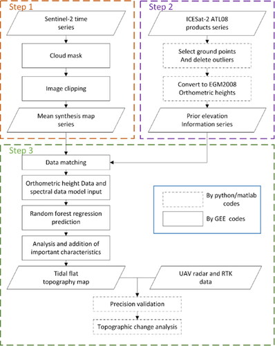
For each Sentinel-2 image in the study area, clouds and shadows are first removed using the quality control band (QA60) provided by the GEE to produce clear observations (Gorelick et al. 2017). The area between the high and low tide lines extracted by the Improved Spectral Water Index (IWI) and Otsu methods (Tang et al. 2022) is considered to be the intertidal extent of the study area. The IWI and Otsu methods have been proven to be highly accurate for waterline extraction. Short-term intertidal extent changes within 5 years are minimal and can be neglected, which means the extracted study area is fixed (Zhang, Xu, et al. 2022). Therefore, we use the area between the low tide line and the high tide line extracted based on remote sensing as the intertidal zone. Since different spectral information as input to the RF model may result in different inversion accuracy of the model, multiple images of the same area over the course of a year are used to explore the effect of changes in spectral information on the accuracy of the model. In addition, Sentinel-2 and ICESat-2 data are used to determine the correlation, water index (the normalized difference water index [NDWI]) by McFeeters (1996), water transparency index (Secchi disk depth [SDD]) by Yang, Yu, et al. (2021) with an RMSE of 0.22 m and suspended sediment concentration index (SSC) by Li et al. (2021) with an RMSE of 42.16 mg/L. These parameters are then added for model training to improve the accuracy of the model. The analysis of feature importance ranking shows that the features we introduced contribute to the model and help improve the accuracy. Since the intertidal zone changes constantly, spectral differences are used to capture these changes. Therefore, we introduce the image time-phase (TP) information for the model (Casas et al. 2014; Zhu et al. 2021), using the ratio between different TP bands as a parameter (McFeeters 1996; Zhu et al. 2021) that is calculated from the mean value of all bands based on pixels. Table 1 is a list of model parameters. All data in the table have been resampled to a spatial resolution of 10 m. The parameters SDD, NDWI and SSC are calculated from the corresponding bands of Sentinel 2 data. In the DATA_TP parameter, ${\mathit{Data}}_{x1}$ and ${\mathit{Data}}_{x2}$ represent two sets of data collected at different times for the same feature (such as ${\mathrm{band}1}_{\mathrm{time}1\mathrm{ }\mathrm{data}1}/{\mathrm{band}1}_{\mathrm{time}2\mathrm{ }\mathrm{data}},$ ${\mathrm{SDD}}_{\mathrm{time}1\mathrm{ }\mathrm{data}1}/{\mathrm{SDD}}_{\mathrm{time}2\mathrm{ }\mathrm{data}}$). All spectral bands, as well as SDD, NDWI and SSC, are calculated for the DATA_TP parameter. Pelletier et al. (2016) have indicated that RF parameters have little impact on model accuracy. So, the number of trees is set as 300, the minimum number of leaf nodes, the bag per tree and the randomization seed are set as default parameters in the GEE for the RF parameters. Additionally, the importance score of the parameters can be calculated by using the ‘explain’ function in the GEE. The feature importance score is not fixed, but varies with model input parameters and can express the degree of importance of the feature. The higher the feature importance score, the greater the importance and contribution of the feature to the model.

Table 1. Feature parameters for the model.

Feature name	Source or calculation formula
Band i (i = 1,…,12)	Sentinel 2 SR
Band 8 A	Sentinel 2 SR
SDD	$-5.838*\log \left(\frac{{\mathit{Band}}_4}{{\mathit{Band}}_1}\right)*\log \left(\frac{{\mathit{Band}}_4}{{\mathit{Band}}_2}\right)*\log \left(\frac{{\mathit{Band}}_3}{{\mathit{Band}}_4}\right)+1.101$
NDWI	$\frac{{\mathit{Band}}_3-{\mathit{Band}}_8}{{\mathit{Band}}_3+{\mathit{Band}}_8}$
SSC	$1.101*\frac{{\mathit{Band}}_4}{{\mathit{Band}}_3}+11.262*{\mathit{Band}}_8+0.76$
DATA_TP	$\frac{{\mathit{Data}}_{x1}}{{\mathit{Data}}_{x2}}$

Since the ICESat-2 ATL08 product is based on WGS84 ellipsoidal heights, not orthometric heights, the EGM2008 gravity model is used to calculate elevation anomalies and then correct them to the orthometric heights to unify the datum. The ATL08 land and vegetation height product are produced from the level 2 product ATL03 dataset using a signal finding approach, resulting in a total of three levels of geolocation photon classification for the ATL03 product: ground (1), canopy (2) and top of canopy (3) (Neumann et al. 2020). We filter all geolocated ATL08 photons with ground markers that match the intertidal region by location and quality information. After deleting certain parameter values according to the overall root mean square criteria provided by the data producer, the orthometric height of the lidar within the pixel grid is obtained. The acquired mean spectral image values with the ATL08 photon data are fed into a constructed RF regression model for training purposes, and the optimized model is used to generate intertidal topography based on orthometric height. Validation data are obtained from the UAV LiDAR data and handheld RTK altimetry data collected in the field in September 2022. Differential change analysis is a commonly used tool to detect topographic changes (Cham et al. 2020). In order to more clearly depict the topographic changes, we use the coefficient variation (CV) (Wang, Bi, et al. 2023) and the slope of change (Slope) (Jin et al. 2020) to calculate multi-year intertidal topographic changes. CV is the ratio of the standard deviation of the original data over the average of the original data, which can be used to measure the degree of variation of the data. Slope is the slope of the linear fitting function of the original data, which can be used to characterize the rate and trend of data changes. We use the bilinear resampling method to scale up the spatial resolution of CV and Slope from 10 to 500 m for better display of the topography changes.

2.2. Study area and data

Only the southern mudflat intertidal zone of Jiangsu is chosen due to the severe erosion and narrow tidal flats in the northern part (Chen et al. 2018; Wang, Liu, et al. 2019; Xu et al. 2016). The area has a unique underwater radiating sandbar in the world with a length of about 200 km in the north-south direction and a width of about 90 km in the east-west direction, which has been formed by the action of the advancing tidal wave system in the East China Sea and the rotating tidal wave system in the Yellow Sea. The area also has a high concentration of suspended sediment in the offshore waters due to the influence of the incoming sediment from the old Yellow River Channel, and the mudflats have experienced an expansion trend in recent decades (Wang, Liu, et al. 2019). The mudflats in this region can reach a maximum difference of 6 m in tidal level. The tide in the area can reach a maximum of 6 m and the maximum tidal velocity can reach 3 m/s, which is a typical semi-diurnal tidal type (Liu et al. 2012).

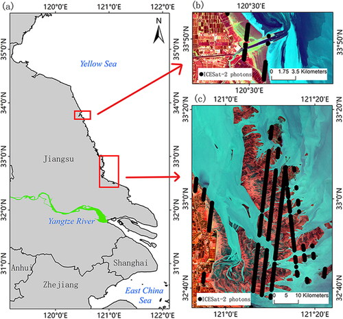
The remote sensing imagery is obtained from Sentinel-2 images with less than 5% cloud cover between 1 January 2019 and 1 October 2022, and the ICESat-2 ATL08 product is screened during the same period in the study area shown in Figure 2. The image spectral data and positioning photon data are then used to construct the RF regression models to invert the intertidal topography. The model-based inversion of the intertidal topography is validated using unmanned airborne high-resolution LiDAR and handheld RTK altimetry data acquired in September 2022. The airborne LiDAR data in Las format and the RTK altimetry data are converted to a 10 m spatial resolution raster format and a uniform datum using the EGM2008 gravity model is used to validate the accuracy of the inversion topography. The mean absolute error (MAE), root-mean-square error (RMSE) and coefficient of determination (R²) are used as the validation criteria (Wang, Wen, et al. 2022).

Figure 2. Overview of the study area; (a) shows the general location of the study area, (b) and (c) are Sentinel-2 images on 18 February 2020 and 13 April 2020, respectively, the names of the areas in (b) and (c) are Sheyang estuary and Radiation Sandbar, respectively, which belong to the wider area of intertidal mudflats in Jiangsu, and the intertidal mudflats in Jiangsu north of Sheyang estuary are gradually decreasing in extent, the black dot pixels in (b) and (c) are schematic diagrams of some location points of ICESat-2 photon data in 2022 located in the intertidal mudflat area.

3. Results

3.1. Model building

The intertidal mudflats are ‘hidden’ when the tide is in motion. The tidal movement in the study area is typical of a semi-diurnal tidal pattern, in which the subsurface features are highly variable in terms of image observations. In order to investigate the influence of different spectral information on the model, we select nine images of the radiated sandbar region (Sentinel-2 frame number: T51SUS) in 2020 as shown in Figure 3. To build time phase information, these nine images are also synthesized to obtain the mean original spectral band for model input in model training for comparison with the results based on different grouping as well as individual images. The grouping information and model training results are shown in Table 2. Each group of data in Table 2 is mutually independent. For each input of spectral information, the model uses the synthesized mean of each group of images by pixel and calculates the NDWI, SSC, SSD and TP information using the method described in Section 2.1. The elevation information inputted into the model each time is the surface elevation of all ICESat-2 data filtered out in 2020.

Figure 3. Sentinel-2 of T51SUS frame number image in 2020; image RGB band settings corresponding to band 8, band 3 and band 2 stretched display; time stamp in the upper right corner of each image is the imaging time.

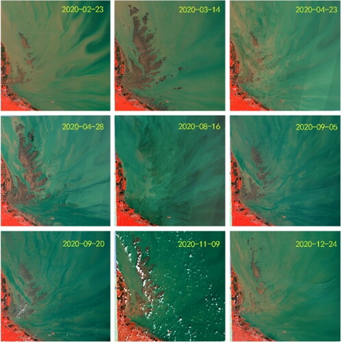
Table 2. Training results of different image set models.

Time (2020)	02/23-03/14	03/14	04/23	08/16	03/14-04/28	02/23-08/16	09/20-12/24	11/09	01/01-12/31
Number of images	2	1	1	1	3	5	3	1	9
MAE (m)	0.33	0.37	0.27	0.24	0.34	0.31	0.31	0.33	0.3
RMSE (m)	0.43	0.47	0.38	0.35	0.43	0.4	0.4	0.43	0.39
R^2	0.79	0.74	0.83	0.85	0.78	0.81	0.82	0.78	0.82

Four sets of single scene images (03/14, 4/23, 8/16 and 11/09) are used to analyse the accuracy of the model when the mudflats are exposed or submerged. Three sets of mean synthetic images (02/23-03/14, 03/14-04/28 and 02/23-08/16) are used to analyse the impact of mean value spectrum on the model under exposure and inundation of mudflats. The 02/23-03/14 group images are used to investigate the equilibrium state of exposure and inundation. The 02/23-08/16 group images are used to examine the inclination of exposure and inundation to the inundation state, and the 03/14-04/28 group images are used to study the exposure and inundation tendency to the exposure state. The 09/20-12/24 group mean composite image is used to analyse the effect on the model accuracy of different amount of data in each pixel of the composite image when some of the data after cloud removal are missing. The 01/01-12/31 combined images are mean composites of all available images that represent the superposition of all scenarios, including areas of missing data, inundated and exposed mudflats. As can be seen from Table 2, the correlation between the model accuracy and the number of images is not significant evident by roughly the same MAEs and RMSEs among different image groups. The model coefficient of determination R² for all the models is greater than 0.74 (sample N = 10,530), the RMSE is smaller than 0.47 m and the MAE is below 0.37 m. According to the comparative analysis of four groups of single scene images, the model accuracy is higher when the mudflats are submerged, and the spectral data loss after cloud removal increases the model error when the image has clouds. At the same time, the RMSE of the 02/23-08/16 group is lower than that of the 03/14-04/28 group and the 02/23-03/14 group, which also proves that the model accuracy is higher when the mudflats are submerged. The comparison between group 09/20-12/24 and group 11/09 shows that the synthetic image can reduce the error caused by cloud image to some extent. By comparing the results of the 01/01-12/31 group and other groups, the RMSE and MAE are 0.04 and 0.06 m higher than the optimal model and 0.08 and 0.07 m lower than the worst model. We believe that with the increase of the number of images, the accuracy of the model has not decreased much. Compared with the 03/14 group, the accuracy of the model has been significantly improved. The larger the area of waterbody covering the mudflat, the higher the accuracy of topography inversion using spectral information. After using the mean value method to merge the mixed spectra of a large number of mudflats or mudflats and waterbody, the maximum reduction of RMSE of the model is 20% compared with the 01/01-12/31 group and the 08/16 group. Although this method leads to a slight decline in the model accuracy, it is simpler to build for a wide range of study areas, especially when the range of the study area exceeds the width of the images used for 3–5 scenes. The determination of the spectral information of the image overlap area will be more unified and efficient. There are ten Sentinel-2 images with different frame numbers in the GEE in the study area. It is more convenient and efficient to synthesize the spectral information of all available images using the mean method. Therefore, the 01/01-12/31 group of data is most suitable, and the subsequent model improvement is conducted by analysing the correlation between the multispectral band values and the model prediction values (Figure 4).

Figure 4. Correlation coefficient between predicted values from respective bands and observed value, Band1,…, Band12 represent Sentinel-2 multispectral bands, Obs is ICESat-2 photon orthometric heights.

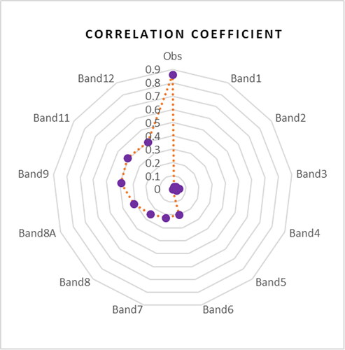
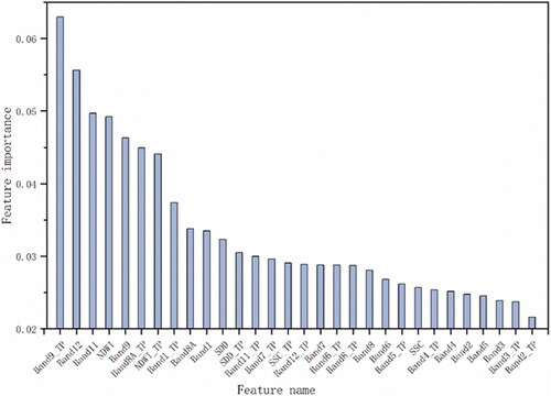
As can be seen from Figure 4, the correlation coefficient between each band and the predicted values does not exceed 0.5, while the correlation coefficient between the model inversion results and the observed values is higher than 0.8. Combining Figure 4 with Table 2, we find that the correlation between the lower reflectance bands and the model predictions is higher and the correlation with the predicted values gradually increases with increasing spectral wavelength. When the tidal flats are inundated with a shallow layer of water, the accuracy of the model is improved seen from Table 2, and the inundated area is still clearly visible as a submerged sandbar (Figure 3), which we believe is related to the suspended sediment and water column in the area. We therefore introduced the NDWI, SDD and SSC parameters for model training. The ratio of the 2020/08/16–2020/03/14 images is used and added to the training of the model. Finally, the model consists of all the spectral bands of Sentinel-2 and four other information bands (i.e. SDD, NDWI, SSC and TP) with a total of 30 bands as the input, and the results show that the model has an R² of 0.89, RMSE of 0.31 m, MAE of 0.22 m and a sample size of N = 10,530, which is a significant improvement (RMSE decreased by 0.08 m, MAE decreased by 0.08 m and R² increased by 0.07) in accuracy compared to the original model. The ranking of importance of the model inputs is shown in Figure 5. This may explain the reason why the topography inversion error is smaller when the tidal flat is submerged, and the contribution of the low reflectivity band of the water body increases when the inundation image is added. The results in Figure 5 show that the TP, NDWI, SSC and SDD all play a crucial role in the improvement of the model performance.

Figure 5. Feature importance ranking of model input parameters. Bandi_TP (i = 1,…,12,8 A) indicates the time-phase difference information for the band; the data has been normalized.

3.2. Intertidal topographic results

The model validation results for the inversion of the complete intertidal topography are shown in Figure 6. The comparison and difference between the topography from the model predictions and the actual topography from RTK and UAV LiDAR data are shown in Figure 7.

Figure 6. Validation of model predictions against ICESat-2 input data, with the color bar showing higher values for denser concentrations of points, and (a), (b), (c) and (d) representing the validation of intertidal topographic inversion predictions against ICESat-2 data for 2019, 2020, 2021 and 2022 respectively.

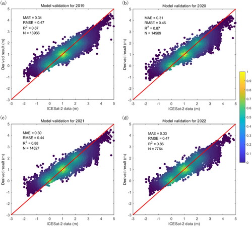
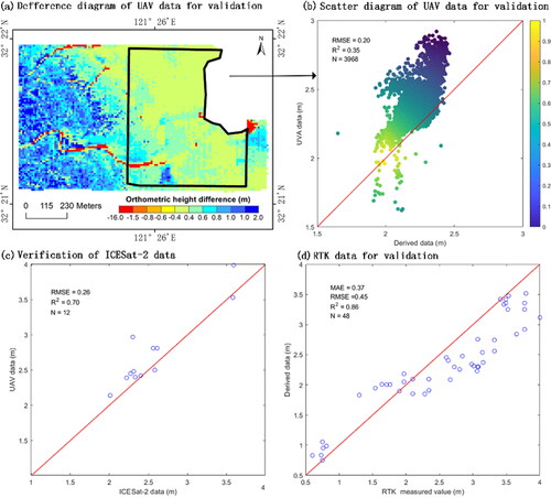
Figure 7. Estimated intertidal terrain accuracy assessment. (a) is a map of the inverse terrain and UAV LiDAR data verification; the calculated result is the difference between the UAV measured terrain and the inverted terrain, with a uniform spatial resolution of 10 m; (b) is a scatter diagram of the UAV data for validation, excluding the data from tidal trenches; (c) is a scatter diagram of verification of ICESat-2 data; (d) is a scatter diagram of RTK data for validation.

From Figure 6(a–d), we can see that the R² of the model training results for each year is greater than 0.85, the RMSE is less than 0.5 m, and the MAE is less than 0.4 m. However, the model overestimates the low value areas and underestimates the high value areas. The underestimation is concentrated in the intertidal vegetation area and the overestimation is concentrated in the area where the tidal trench is located. As the intertidal vegetation areas are closer to the shore, they are inundated by tidal water for a short time, and the tide water usually flows into the coast through the tidal trench during high tide, and sometimes the tide water only exists in the tidal trench below the beach level. The intertidal zone in Jiangsu has the largest amount of intertidal Spartina alterniflora, and a few Suaeda salsa and Phragmites australis (Zeng et al. 2022). As the plants are higher and the water surface is lower, it is difficult for remote sensing satellites to penetrate through to obtain optical information under plants. The mixed spectrum of 10 m spatial resolution in this region has a high consistency with the vegetation spectrum, and the spectral information is less affected by water, resulting in the underestimation of the topography of the vegetated area. Since the edge of the mudflat is greatly affected by water, the mixed spectrum tends to be mainly from water and the spectral changes of the continuous phase are slight, which leads to the overestimation by the model. In addition, the tidal trenches are typically deep and have been submerged for years. The spectral information, therefore, varies less and satellites are more difficult to penetrate underwater to obtain underwater spectral information, also leading to overestimation.

As seen in Figure 7(a), which shows the difference between the UAV measured topography and the inverted topography, the topographic error decreases from left to right. The underlying surface of the acquisition area is vegetated and intertidal mudflats from left to right and the mudflats area RMSE is 0.20 m (see Figure 7(b)), which is obtained by removing the error of the tidal trenches and calculating the partial error of the tidal trenches with an RMSE of approximately 1.10 m. The closer it is to the vegetation area as a whole, the greater the error in the inversion results, with the largest error at the tidal trenches. Figure 7(c) is a scatter diagram of UAV and ICESat-2 data. Due to the trajectory of ICESat-2 data, there is less overlap with UAV data. The RMSE of 0.26 m shows that the data can be used for terrain inversion of intertidal zone. From Figure 7(d), we can see that the inverted topography is in good agreement with the RTK-measured data, mainly at the junction of the mudflats and the vegetation zone. The RMSE is 0.45 m due to the large difference in spatial resolution between the RTK and inversion data, which is difficult to correct. The RTK data collection area is mainly composed of mixed pixels of vegetation and light beach, which may also lead to some errors. Therefore, the topographic inversion results from our method are better for the intertidal mudflats than the submerged tidal trenches or vegetation growth areas.

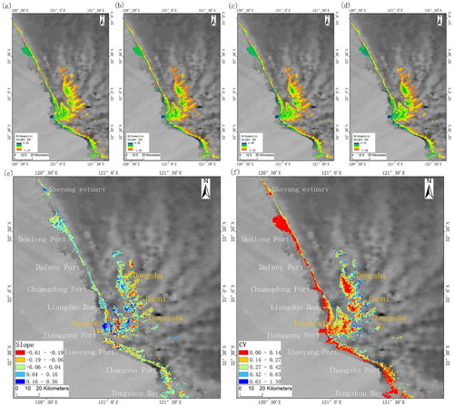
Figure 8(a–d) shows the inversion results of intertidal topography for 2019–2022 and Figure 8(e, f) plots the results of the CV and the Slopes of change, derived from CV and Slope resampling with a spatial resolution of 10 m. The topography has changed little during the 4-year period. The most noticeable changes have been on the seaward side of the intertidal zone, with the fastest increase in the south-western part of the radiation sandbar and the Sheyang estuary channel island embankment and the fastest decrease in the middle of radiation sandbar. The southwestern part of the radial sandbar is a strip mud area, where the combined effect of the East China Sea forward tidal system and the Yellow Sea rotating tidal system results in larger and stronger tidal currents, making the area more complex than the surrounding area (Chen et al. 2007; Wang, Liu, et al. 2019). The construction of island dikes in the Sheyang estuary channel embankment has slowed down the coastal currents (Wang, Chen, et al. 2019). The sediment transport and flow in the direction parallel to the shoreline become slower, which enhances the sediment transport parallel to the island embankment and the topography on the two sides of the embankment has increased slightly. The topography from Doulong Port to Liangduo Dam has almost no change, and the overall topography from Jianggang Port to Changsha Port has a slight decrease trend. In addition, the high concentration of suspended sediment in Jiangsu coastal water and the frequent sediment exchanges between the sea and land in the direction perpendicular to the coastline have resulted in a greater sedimentation trend closer to the high-tide line.

Figure 8. Intertidal topography inversion image. Figure 8(a–d) is the inverted intertidal topography in 2019, 2020, 2021 and 2022 with a spatial resolution of 10 m; Figure 8(e) is the slope of the topography in 2019–2022 with a spatial resolution of 500 m and Figure 8(f) is the variation coefficients of the topography in 2019–2022 with a spatial resolution of 500 m; the background of all images is from GEBCO data in 2022 (Group 2022).

4. Discussion

We propose a fusion of ICESat-2 and Sentinel-2 datasets as input to a RF learning model to construct higher contribution inversion features for the inversion of non-optical intertidal topography and compare the results to the original spectral bands. The study demonstrates the potential of this method for topographic derivation of intertidal areas. Since the method relies entirely on satellite remote sensing data, there is a great potential for a wide range of data sources and a possibility of remote sensing inversion of global intertidal topography. The method is then applied to invert the intertidal topography of largest intertidal area in Jiangsu coastal area in China. The results show that the intertidal topography in the area has changed slightly over the years in a slow siltation pattern, with the topography near the ocean side changing more significantly than the land side.

As shown in Figure 7, the predicted mudflats topography is generally consistent with the RTK data and the UAV LiDAR data, but with greater variation in vegetated areas and tidal trench, which is related to the difficulty of spectroscopy penetrating underwater and terrestrial vegetation to directly obtain the topography. We believe that the proposed TP could be a very important characteristic, especially in dynamic areas such as the intertidal zone. The vegetation in the intertidal zone of Jiangsu province is characterized by a salinity gradient from the sea to the land, with Suaeda salsa, Spartina alterniflora and Phragmites australis growing successively. Except for Suaeda salsa, which is short and scattered, the vegetation has similar growth patterns during the mature season, reaching a maximum height of 2 m. The accuracy of lidar data for terrain under mature Suaeda salsa plants may be better than for terrain under Spartina alterniflora and Phragmites australis. It is difficult to obtain reflectance information of the ground under these vegetations using optical images. Because the growth patterns of the vegetation vary at different times, features (TP) from different times were proposed to eliminate the influence of vegetation and invert the terrain. The limitations of this study may lie in the lack of using the maximum seasonal difference (such as winter and summer). The study area requires multiple Sentinel-2 images. The results show that the RMSE of the composite image model is between that of the worst and best single image models (Table 2), and there is no significant correlation between the number of composite images and RMSE (p > 0.01). Using an annual mean composite image may not necessarily lead to a significant decrease in accuracy. The study did not address photon filtering and terrain inversion correction in tidal trenches, which may be the biggest source of error. After removing the tidal gully differences, the RMSE is only 0.20 m. Without removing the tidal trenches differences, the RMSE is about 1.10 m, which has a high correlation with the fixed study area. In future studies, the identification of tidal gullies in the intertidal zone will help us improve this study.

This study demonstrates that the inclusion of TP, NDWI, SDD and SSC in the model can improve the model accuracy (RMSE decreased by 20%). TP and NDWI contribute the most to the accuracy improvement, followed by SDD. The intertidal zone of Jiangsu province has a high concentration of suspended sediment, and the tidal flats still have water content after ebb tide. These indicators can reflect some features of the study area. The accuracy of the RF model is affected by the input characteristic features, as well as the known terrain height (ICESat-2 in this study). Due to the 90-d observation period of ICESat-2, which is much longer than the tidal period, the accuracy of the model may decrease due to the non-uniform data collection time. Since the RMSE of UAV data is 0.26 m as shown in Figure 7(c), there may be some degree of error.

The method in this study inverts intertidal mudflats topography with an RMSE of 0.20 m. In addition, Zhou et al. (2021) inverted the intertidal terrain of the offshore sandbanks with an RMSE of 0.54 m, Zhang, Wu, et al. (2022) inverted topography of the tidal flats of the Yangtze Estuary with an MAE of 0.15 m, the RMSE of Xu et al. (2022) and the MAE of Zhang, Xu, et al. (2022) are 0.23 and 0.29 m, respectively, for the inversion of topography of the tidal flat in Jiangsu. Compared with the errors of these studies, the error of this study is within an acceptable range. This research demonstrates the ability to use spectral information to invert intertidal topography, especially for intertidal mudflats, which can be useful for intertidal topography monitoring and investigation of human-terrestrial relationships. The ease with which the intertidal zone can be inundated makes it difficult to obtain topographic data directly from satellite data. Intertidal topographic datasets are still missing for many regions of the globe currently, and this study may bring a new perspective to accelerate the generation of datasets. This is closely related to global sea level rise, coastal vulnerability assessment, wetland protection and port siting. Furthermore, with the massive amount of data and maximum global scale processing of the GEE cloud platform, there is great potential for the method to be extended to MODIS or Landsat series satellites.

5. Conclusions

In this study, a new method is developed for the extraction of mudflat topography, which reduces the cost and improves the efficiency by replacing a large number of in-situ observation data with remote sensing data. We use a large number of ICESat-2 lidar and Sentinel-2 data to retrieve the mudflat topography using a RF regression model. The main conclusions can be summarized as follows.

1. The larger the area of waterbody covering the mudflat, the higher the accuracy of topography inversion using spectral information. After using the mean value method to merge the mixed spectra of a large number of mudflats or mudflats and waterbody, the accuracy of the model decreases slightly (the RMSE increases by a maximum of 20%). However, it is simpler to build a model for a wide range of study area, and the determination of the spectral information of the image overlap area is more unified and efficient.

2. TP is an important index for improving model accuracy. Since intertidal zone is dynamic, whereas remote sensing data are static, it is important to add a time change index to the static remote sensing data to represent the change of time phase. The NDWI is another index that can be used to improve model accuracy.

3. The scaling method is used to upscale fine-resolution topography to large-scale topography. The study shows that the topography has changed little during the 4-year period. The most noticeable changes occur on the seaward side of the intertidal zone with the fastest increase in the south-western part of the radiation sandbar and the Sheyang estuary channel island embankment. The topography from Doulong Port to Liangduo Dam has almost no change, and the overall topography from Jianggang Port to Changsha Port has decreased slightly.

Author contribution statement

The first draft was prepared by Wei Tang. All authors provide data and actively participate in the revision.

Acknowledgements

We thank the National Natural Science Foundation of China grant, No. 42130405, and the Innovative and Entrepreneurial Talent Program of Jiangsu Province grant, No. R2020SC04.

Disclosure statement

The authors declare that they have no known competing financial interests or personal relationships that could have appeared to influence the work reported in this article.

Data availability statement

Data available on request from the authors.

Additional information

Funding

This work was supported by the National Natural Science Foundation of China grant, No. 42130405, and the Innovative and Entrepreneurial Talent Program of Jiangsu Province grant, No. R2020SC04.

References

- Andriolo U, Almeida LP, Almar R. 2018. Coupling terrestrial LiDAR and video imagery to perform 3D intertidal beach topography. Coastal Eng. 140:232–239.
- Beijma S, Comber A, Lamb A. 2014. Random forest classification of salt marsh vegetation habitats using quad-polarimetric airborne SAR, elevation and optical RS data. Remote Sens Environ. 149:118–129.
- Bishop-Taylor R, Sagar S, Lymburner L, Beaman RJ. 2019. Between the tides: modelling the elevation of Australia’s exposed intertidal zone at continental scale. Estuarine Coastal Shelf Sci. 223:115–128.
- Breiman L. 2001. Random forests. Mach Learn. 45(1):5–32.
- Breiman L, Friedman JH, Olshen RA, Stone CJ. 2017. Classification and regression trees. Abingdon: Routledge.
- Brunier G, Oiry S, Lachaussée N, Barillé L, Fouest VL, Méléder V. 2022. A machine-learning approach to intertidal mudflat mapping combining multispectral reflectance and geomorphology from UAV-based monitoring. Remote Sens. 14(22):5857.
- Casas A, Riaño D, Ustin S, Dennison P, Salas J. 2014. Estimation of water-related biochemical and biophysical vegetation properties using multitemporal airborne hyperspectral data and its comparison to MODIS spectral response. Remote Sens Environ. 148:28–41.
- Cham DD, Son NT, Minh NQ, Thanh NT, Dung TT. 2020. An analysis of shoreline changes using combined multitemporal remote sensing and digital evaluation model. Civ Eng J. 6(1):1–10.
- Chen J, Wang Y, Zhang R, Lin X. 2007. Stability study on the Dongsha sandbanks in submarine radial sand ridges field off Jiangsu coast. Ocean Eng. 25:105–113.
- Chen W, Zhang D, Cui D, Lv L, Xie W, Shi S, Hou Z. 2018. Monitoring spatial and temporal changes in the continental coastline and the intertidal zone in Jiangsu province, China. Acta Geograph Sin. 73:1365–1380.
- Costanza R, d‘Arge R, de Groot R, Farber S, Grasso M, Hannon B, Limburg K, Naeem S, O'Neill RV, Paruelo J, et al. 1997. The value of the world’s ecosystem services and natural capital. Nature. 387(6630):253–260.
- Dai W, Li H, Zhou Z, Cybele S, Lu C, Zhao K, Zhang X, Yang H, Li D. 2018. UAV photogrammetry for elevation monitoring of intertidal mudflats. J Coast Res. 85:236–240.
- Ebrahimy H, Aghighi H, Azadbakht M, Amani M, Mahdavi S, Matkan AA. 2021. Downscaling MODIS land surface temperature product using an adaptive random forest regression method and Google Earth Engine for a 19-years spatiotemporal trend analysis over Iran. IEEE J Sel Top Appl Earth Observ Remote Sens. 14:2103–2112.
- Erlandson JM. 2008. Racing a rising tide: global warming, rising seas, and the erosion of human history. J Island Coast Archaeol. 3(2):167–169.
- Gao S. 2009. Modeling the preservation potential of tidal flat sedimentary records, Jiangsu coast, eastern China. Cont Shelf Res. 29(16):1927–1936.
- Gao W, Shen F, Tan K, Zhang W, Liu Q, Lam NS, Ge J. 2021. Monitoring terrain elevation of intertidal wetlands by utilising the spatial-temporal fusion of multi-source satellite data: a case study in the Yangtze (Changjiang) Estuary. Geomorphology. 383(2021):107683.
- Gorelick N, Hancher M, Dixon M, Ilyushchenko S, Thau D, Moore R. 2017. Google earth engine: planetary-scale geospatial analysis for everyone. Remote Sens Environ. 202:18–27.
- Group, G.C. GEBCO_2022 Grid. 2022. DOI:10.5285/e0f0bb80-ab44-2739-e053-6c86abc0289c
- Henriques M, Catry T, Belo JR, Piersma T, Pontes S, Granadeiro JP. 2022. Combining multispectral and radar imagery with machine learning techniques to map intertidal habitats for migratory shorebirds. Remote Sens. 14(14):3260.
- Heygster G, Dannenberg J, Notholt J. 2010. Topographic mapping of the German tidal flats analyzing SAR images with the waterline method. IEEE Trans Geosci Remote Sens. 48(3):1019–1030.
- Hsu HJ, Huang CY, Jasinski M, Li Y, Gao H, Yamanokuchi T, Wang CG, Chang TM, Ren H, Kuo CY, et al. 2021. A semi-empirical scheme for bathymetric mapping in shallow water by ICESat-2 and Sentinel-2: a case study in the South China Sea. ISPRS J Photogramm Remote Sens. 178:1–19.
- Jin K, Wang F, Han JQ, Shi SY, Ding WB. 2020. Contribution of climatic change and human activities to vegetation NDVI change over China during 1982-2015. Acta Geograph Sin. 75:961–974.
- Kuter S. 2021. Completing the machine learning saga in fractional snow cover estimation from MODIS Terra reflectance data: random forests versus support vector regression. Remote Sens Environ. 255:112294.
- Li P, Ke Y, Wang D, Ji H, Chen S, Chen M, Lyu M, Zhou D. 2021. Human impact on suspended particulate matter in the Yellow River Estuary, China: evidence from remote sensing data fusion using an improved spatiotemporal fusion method. Sci Total Environ. 750:141612.
- Lin Y, Fan J, Wen Q, Liu S, Li B. 2016. Primary exploration of ecological theories and technologies for delineation of ecological redline zones. Acta Ecol Sin. 36:1244–1252.
- Liu Y, Li M, Cheng L, Li F, Chen K. 2012. Topographic mapping of offshore sandbank tidal flats using the waterline detection method: a case study on the Dongsha Sandbank of Jiangsu Radial Tidal Sand Ridges, China. Mar Geod. 35(4):362–378.
- Liu Y, Li M, Zhou M, Yang K, Mao L. 2013. Quantitative analysis of the waterline method for topographical mapping of tidal flats: a case study in the Dongsha Sandbank, China. Remote Sens. 5(11):6138–6158.
- Luijendijk A, Hagenaars G, Ranasinghe R, Baart F, Donchyts G, Aarninkhof S. 2018. The state of the world’s beaches. Sci Rep. 8(1):1–11.
- Ma Y, Xu N, Liu Z, Yang B, Yang F, Wang XH, Li S. 2020. Satellite-derived bathymetry using the ICESat-2 lidar and Sentinel-2 imagery datasets. Remote Sens Environ. 250:112047.
- Markus T, Neumann T, Martino A, Abdalati W, Brunt K, Csatho B, Farrell S, Fricker H, Gardner A, Harding D, et al. 2017. The Ice, Cloud, and land Elevation Satellite-2 (ICESat-2): science requirements, concept, and implementation. Remote Sens Environ. 190:260–273.
- McFeeters SK. 1996. The use of the Normalized Difference Water Index (NDWI) in the delineation of open water features. Int J Remote Sens. 17(7):1425–1432.
- Miles A, Ilic S, Whyatt D, James MR. 2019. Characterizing beach intertidal bar systems using multieinethe LiDAR data. Earth Surf Process Landforms. 44(8):1572–1583.
- Neumann T, Brenner A, Hancock D, Robbins J, Saba J, Harbeck K, Gibbons A, Lee J, Luthcke S, Rebold T. 2020. ATLAS/ICESat-2 L2A global geolocated photon data, version 3. Boulder (CO): NASA National Snow and Ice Data Center Distributed Active Archive Center.
- Pelletier C, Valero S, Inglada J, Champion N, Dedieu G. 2016. Assessing the robustness of Random Forests to map land cover with high resolution satellite image time series over large areas. Remote Sens Environ. 187:156–168.
- Sagar S, Roberts D, Bala B, Lymburner L. 2017. Extracting the intertidal extent and topography of the Australian coastline from a 28 year time series of Landsat observations. Remote Sens Environ. 195:153–169.
- Tang W, Zhao C, Lin J, Jiao C, Zheng G, Zhu J, Pan X, Han X. 2022. Improved spectral water index combined with Otsu algorithm to extract muddy coastline data. Water. 14(6):855.
- Tao X, Zhang D. 2013. Inversion of tidal flat elevation based on hyperspectral remote sensing. Adv Mar Sci. 31:498–507.
- Thomas N, Pertiwi AP, Traganos D, Lagomasino D, Poursanidis D, Moreno S, Fatoyinbo L. 2021. Spaceinbois marine sciencengation based on hyperspectral remote sensinguddy coastland sentinelis. Geophys Res Lett. 48(6):e2020GL092170.
- Wang JS, Bi RT, He P, Xu LS, Liu ZC, Cao CB. 2023. Dynamic characteristics of NDVI during main growth seasons in the Chinese Loess Plateau effect by climate change. Chin J Ecol. 42(01):67–76.
- Wang N, Chen K, Lu P, Chen Y, Zhang J, Wang Y. 2019. Impact of a water–sediment regulation scheme on the hydrodynamics and sediment conditions in the Sheyang Estuary. Estuarine Coastal Shelf Sci. 218:349–358.
- Wang X, Wen Z, Liu G, Tao H, Song K. 2022. Remote estimates of total suspended matter in China’s main estuaries using Landsat images and a weight random forest model. ISPRS J Photogramm Remote Sens. 183:94–110.
- Wang Y, Liu Y, Jin S, Sun C, Wei X. 2019. Evolution of the topography of tidal flats and sandbanks along the Jiangsu coast from 1973 to 2016 observed from satellites. ISPRS J Photogramm Remote Sens. 150:27–43.
- Xu F, Tao J, Zhou Z, Coco G, Zhang C. 2016. Mechanisms underlying the regional morphological differences between the northern and southern radial sand ridges along the Jiangsu Coast, China. Mar Geol. 371:1–17.
- Xu N, Ma Y, Yang J, Wang XH, Wang Y, Xu R. 2022. Deriving tidal flat topography using ICESat‐2 laser altimetry and sentinel‐2 imagery. Geophys Res Lett. 49(2):e2021GL096813.
- Yang L, Xiao Y, Jiang J, Chen Y, Gu Y, Zhang S. 2021. Remote sensing method for extracting topographic information on tidal flats using spatial distribution features. Mar Geod. 44(5):408–431.
- Yang L, Yu DF, Gao H, Bian XD, Liu XY, Gai YY, An DY, Zhou Y, Tang SL. 2021. Remote sensing retrieval of secchi disk depth in Jiaozhou Bay using Sentinel-2 MSI image. Infrared Laser Eng. 50:515–521.
- Zeng J, Sun Y, Cao P, Wang H. 2022. A phenology-based vegetation index classification (PVC) algorithm for coastal salt marshes using Landsat 8 images. Int J Appl Earth Obs Geoinf. 110:102776.
- Zhang H, Hu L, Zhang D, Zhou Y, Ma Y, Wang X, Wang Y, Xu M, Xu N. 2021. A method to derive tidal flat topography in Nantong, China using MODIS data and tidal levels. Can J Remote Sens. 47(1):17–32. 10.1080/07038992.2021.18796
- Zhang M, Wu WT, Wang XQ, Sun Y. 2022. Topographic retrieval of the tidal flats in the Yangtze Estuary based on the dynamic tidal submergence. J Geo-Inform Sci. 24:583–596.
- Zhang S, Xu Q, Wang H, Kang Y, Li X. 2022. Automatic waterline extraction and topographic mapping of tidal flats from SAR images based on deep learning. Geophys Res Lett. 49(2):e2021GL096007.
- Zhi C, Wu WT, Su H. 2022. Mapping the intertidal wetlands of Fujian Province based on tidal dynamics and vegetational phonology. Natl Remote Sens Bull. 26:373–385.
- Zhou Y, Zhang D, Deng H, Xu N, Zhang H, Hao X, Shen Y. 2021. The enhanced construction method for intertidal terrain of offshore sandbanks by remote sensing. Haiyang Xuebao. 43(12):133–143.
- Zhu WX, Sun ZG, Li BB, Yang T, Liu Z, Peng JB, Zhu KY, Li SJ, Lou JY, Hou RX, et al. 2021. Analysis of spatial heterogeneity for soil attributes and spectral indices-based diagnosis of coastal saline-alkaline farmland stress using UAV remote sensing. J Geo-Inform Sci. 23:536–549.