BIF-hosted high-grade magnetite iron ore targeting by hyperspectral wavelength mapping of chlorite: case study of Qidashan Iron Mine, northeast China

Abstract

There are two kinds of chlorites occurred in Anshan area, among which the hydrothermal Fe-chlorite with longer Fe-OH wavelength is spatially related to the high-grade magnetite ore, meaning that wavelength mapping of chlorites can be used to target the BIF-hosted high grade iron ore. In this article, quadratic polynomial, cubic spline, and quartic polynomial method were used to interpolate the absorption wavelength near 2250 nm of China ZY1-02D satellite hyperspectral image. The result of quadratic polynomial is continuous without data overlapping or intervals, thus most suitable for discrimination of the chlorites. The field truth shows that the spatial distribution of Fe-chlorite, validated by XRD analysis, is not only in accordance with that of high grade magnetite ore bodies, but also consistent with the recently discovered concealed iron bonanza. The study shows that hyperspectral remote sensing techniques can play significant role in the exploration of magnetite iron ore in east Liaoning Province.

Keywords:

• High-grade magnetite iron ore
• chlorite
• wavelength mapping
• hyperspectral
• ZY1-02D satellite image

1. Introduction

China has been the largest producer and consumer of crude steel in the world for decades (Zhao et al. 2020; Zheng et al. 2022), however more than 50% of the demand of iron ores were met by foreign sources in recent years (Li H, Yang, et al. 2015). The average ca.34% iron grade of the iron ore in China (Zhang et al. 2014; Li H, Li, et al. 2015), among which the high-grade iron ore (>50% Fe) is estimated to be only 1% of the total iron ore resources, makes the situation worse. Thus, a fast, effective and convenient iron content estimation method is of great help not only to exploration of the high-grade iron ore, but also to the ore-blending during the production of iron mine.

Hyperspectral remote sensing is known for ‘spatially contiguous spectra and spectrally contiguous images’, i.e. each pixel can be regarded as an individual spectrum, which delicately characterize the type, distribution and even the composition of corresponding ground objects. Thanks to Hunt (1977) and Salisbury et al. (1989) and their co-workers (Hunt 1977; Salisbury et al. 1989), the diagnostic features of the main minerals and rocks were systematically determined and made the spectral identification of minerals possible. The hyperspectral methods have been routinely used in the field of drill core and chips, hand specimen, and mine surface (Krupnik and Khan 2019; Ramanaidou et al. 2022). Since 1980s, the airborne hyperspectral had been widely applied to mineral mapping, providing the researchers a quick, large-coverage, but costly technology for mineral exploration (Kruse et al. 2003; Bishop et al. 2018). However, the NASA EO-1 sensor launched in 2000, and the GF-5 and ZY1-02D sensors of China, the PRISMA sensor of Italy and the EnMAP sensor of Germany in recent years, offer geologists the possibility to acquire hyperspectral data worldwide at limited cost, which creates a new era for the geological application of hyperspectral remote sensing technology.

BIF-hosed iron ore deposits represent the world’s largest and highest grade iron ore districts and deposits, and meanwhile account for the majority of current world production (Clout et al. 2005; Hagemann et al. 2016). In most cases, the high-grade iron ore deposits worldwide are originated from supergene or epigenetic hydrothermal enrichment of BIF protore, and mainly composed of hematite and goethite (Clout et al. 2005; Hagemann et al. 2008; Wang E et al. 2014; Li H, Yang, et al. 2015; Hagemann et al. 2016). These iron oxides and/or hydroxides manifest obvious absorption spectral features (Hunt 1971; Clark and Roush 1984; Clark et al. 1990), thus the mineral types, abundance, and boundaries of iron ore can be easily discriminated by satellite image derived spectral signatures (Ganesh et al. 2013; Magendran and Sanjeevi 2013, 2014; Panda et al. 2018; Fonteneau et al. 2019; SrinivasaPerumal et al. 2020). However, the subordinate amounts of high-grade iron ore in China is dominated by magnetite, whether they are of skarn or BIF-related type (Wang E et al. 2014; Zhang et al. 2014; Li H, Li, et al. 2015; Li H, Yang, et al. 2015). As we all know, the magnetite is characterized by surface scattering dominant and high extinction over the entire visible-near infrared-shortwave infrared (0.35-2.5 μm) wavelength range (Izawa et al. 2019), resulting in ‘flat and featureless’ reflectance spectroscopic characteristics (Hunt 1971; Izawa et al. 2019). This means magnetite is difficult to be discriminated by remote sensing method. Fortunately, the coeval chlorite-dominant alteration resulted from hypogene hydrothermal fluid, which was intimately related to the formation of BIF-hosted high-grade iron ore (Sun et al. 2014; Wang E et al. 2014; Li H, Li, et al. 2015; Li H, Yang, et al. 2015; Li L et al. 2016; Li L et al. 2019), exhibits prominent spectral absorption feature, providing an alternative way for magnetite ore targeting.

There are two kinds of chlorites in the districts of iron ore deposits in Anshan area, one of which mainly occurs in BIF and metamorphic wall rocks such as various schist and phyllite, while the other is limited in the hydrothermal alteration rocks peripheral to the high grade magnetite ore. Point measurement by ASD FieldSpec-3 spectrometer and close-range HySpex 320 m imaging system indicated that the former exhibited shorter Fe-OH wavelength, whereas the latter is relatively longer, meaning that the Fe-OH wavelength mapping could be regarded as an explorative tool for the targeting of BIF-hosted high-grade magnetite iron ore (Hao et al. 2020), but as for the space-borne hyperspectral images, there are still several factors need to be considered.

First of all, the spectral resolution of the hyperspectral images is crucial to mineral mapping. In most cases, the FWHM (full width at half maximum) of the diagnostic features of most alteration minerals is ca. 20-40 nm (Hunt 1979), which means the spectral resolution of the selected hyperspectral images should be finer than 20 nm. Furthermore, the low reflectivity of the BIFs and its peripheral ‘dark’ metamorphic and/or chloritic alteration wall rocks will totally affect the SNR of hyperspectral images, i.e. the less-than-optimum data acquisition conditions should be a great challenge for the mineral identification of the space-borne hyperspectral imaging system (Kruse et al. 2003). Finally, the wavelength mapping methods were proven to be effective, robust, reproducible, and accurate enough to distinguish the subtle mineralogical information of the within-species variability (van Ruitenbeek et al. 2006; van der Meer et al. 2018; Hecker, van Ruitenbeek, Bakker, et al. 2019), and most importantly they were considered to be suitable for the discrimination of ‘dark’ targets with shallow absorption features (van Ruitenbeek et al. 2014). However, several algorithms were used for wavelength mapping (Clark 1980; McCord et al. 1981; Kruse 1988; Tong et al. 2006; van Ruitenbeek et al. 2006; Rodger et al. 2012; Tan and Md Ali 2013; Murphy et al. 2014; van Ruitenbeek et al. 2014; Murphy et al. 2015; van der Meer et al. 2018; Hecker, van Ruitenbeek, Bakker, et al. 2019), thus another purpose of the article is to verify which method is optimum for the wavelength mapping of dark chlorites.

Based on the concerns mentioned above, the current study has accessed (1) in-situ investigation of Qidashan open-pit mine; (2) point spectral measurements by ASD Fieldspec-3 spectrometer and images collected by close-range HySpex 320 m spectrometer of selected rock samples; (3) ground-based high resolution apparent susceptibility mapping; (4) XRD analysis of selected iron ore and wall-rock samples; (5) geological logging of working terraces in Qidashan Iron Mine; (6) ZY1-02D satellite hyperspectral images, and aims to determine which method is most suitable for within-species chlorite discrimination by wavelength mapping of ZY1-02D satellite hyperspectral image, and subsequently explain the spatial linkage between BIF-hosted high-grade magnetite iron ore and chloritic alteration rocks and finally discuss the potential application of hyperspectral imaging system in mineral exploration in eastern Liaoning Province.

2. Geological setting

2.1. Regional geology

Qidashan Iron Mine, ca.10 km northeast of Anshan city, lies at northeastern margin of North China Craton (NCC, Figure 1(a)), which is one of the oldest cratonic blocks in the world (Liu et al. 1992; Song et al. 1996; Liu et al. 2008). The strata occurred in Anshan area include two Neoarchean formations: the Yingtaoyuan formation, distributing as N-S and W-E extended, ribbon-shaped narrow greenstone belts, is mainly composed of chloritic schist and phyllite and accounts for most of the iron resources in the studying area, i.e. the so-called N-S iron ore belt and W-E iron ore belt (Zhou 1994); the Dayugou formation, with subordinate amount of BIF resources, scatters in the central part of Anshan area, and mainly consists of chloritic and biotitic schist, locally with some plagioclase amphibolite and granulite. The Proterozoic strata mainly locate in the eastern and southern part of the studying area, and consist of sericite schist, marble, quartz sandstone and shale. The Cambrian shale and limestone unconformably layer on the Proterozoic rocks. The Quaternary unconsolidated sediments widely spread in the western depression and other low-lying part of Anshan area (Figure 1(b)).

Figure 1. (a) Distribution of the basement rocks in the North China Craton and the distribution of the Eastern and Western blocks and the Central zone (Zhao G et al., 2001). (b) Sketch map of regional geology of Anshan area. The BIF-bearing Neoarchean ribbon-shaped greenstone belts distribute as N-S and W-S iron belts, enclosed by granitic rocks of various ages.

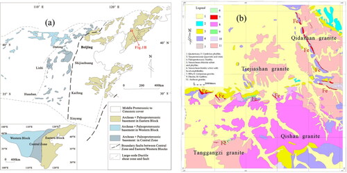
Magmatic rocks dominate approximately 50% of the total surface coverage of the studying area, including Archean Tiejiashan granite, Qidashan granite, Tanggangzi granite, and Mesozoic Qianshan granite (Figure 1(b)). The latest SHRIMP U-Pb age of Tiejiashan granite is 2.95 ∼ 3.0Ga (Bao et al. 2020), which is obviously earlier than the BIF-bearing Archean greenstone belt (Li L et al. 2016). The granite is regarded as the oldest pluton in Anshan area and spatially acts as the western boundary of N-S iron ore belt. Qidashan granite lies to the east of the N-S iron ore belt, and locally intruded into the iron ore or partially assimilated the Archean strata, resulting in the direct contact of granite with the BIF ore. This means Qidashan granite was formed a bit later than BIF or reactivated after the formation of BIF. As for Tanggangzi granite, there are few detailed data about the geochronology and geochemistry till now, however the characteristics of rock mass are similar to those of Qidashan granite, and are considered to be coeval with Qidashan granite (Zhou 1994). Qianshan granite, formed at ca.130.2Ma, evidently intruded into the Archean granite and Precambrian strata (Bora et al. 2013), but had little effect on the continuity of the BIFs.

Structures were well developed in Anshan area (Zhou 1994; Liu et al. 2017, 2019). The detailed macro-structure analysis reveals that the overall structures in Anshan area manifest as ‘dome and keel structure’ tectonic pattern, i.e. Tiejiashan granite exhibits as dome, and the N-S and W-N iron ore belts as steep-dipping-slip ductile shear zone, which constitutes the overall tectonic framework in Anshan area (Liu et al. 2017, 2019). The coeval transverse faults, reactivated at ca.18.6Ga, were of crucial importance to the BIF-hosted high-grade iron ore (Li H, Yang, et al. 2015; Li L et al. 2019). The NE, NW and W-E extending Mesozoic faults were limited in Qianshan area (Figure 1(b)).

2.2. Deposit geology

Qidashan Iron Mine is one of the most important iron resource bases for An Steel Co., meanwhile it is also the second largest BIF-hosted high-grade iron ore deposit in Anshan-Benxi area (Li H, Yang, et al. 2015). The open-pit mine was composed of two mining districts: the northern mining district includes five sub-districts, i.e. Beiyishan, Beiershan, Beisanshan, Beisishan and Xishilazi; the southern mining district consists of No.1, No.2 and No.3 sub-district (Figure 2).

Figure 2. Sketch Geology map of Qidashan Iron Mine.

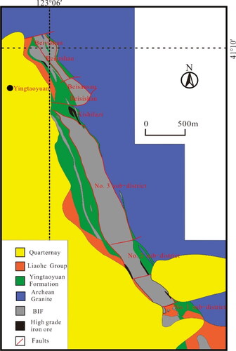
The originally single BIF ore body was cut into several pieces by the transverse faults, resulting in the minor variations of strike and dip angle. As a whole, the iron ore bodies in Qidashan mining district is stratiform, with a 4900 m length and an average 200 m thickness. The overall strike of ore bodies is 330°, dip to the southwest with dip angle of 70-90°. The iron ore, commonly with 32% total Fe content, is mainly composed of alternative laminae of magnetite and quartz (Figure 3 (a)), among which magnetite are often oxidized into martite near the surface. Note that there are usually small amount of chlorite and sericite in the ‘dark’ iron laminae (Figure 3 (b)). Occasionally there are some epigenetic carbonate (Figure 3 (c)) or sericite (Figure 3 (d)) veinlets crosscutting the BIF ore.

Figure 3. Photomicrograph of iron ore and wall rocks in Qidashan Iron Mine. (a) Alternative laminae of magnetite and quartz in BIF; (b) Pale-green chlorite scattered in BIF ore; (c) epigenetic calcite veinlet crosscutting BIF ore; (d) sericite in BIF ore; (e) high grade magnetite ore; (f) pyrite coexisting with magnetite in high grade iron ore; (g) Pale green chlorite in chlorite quartz schist; (h) strong chloritization peripheral to high-grade iron ore. Mag-magnetite; Q-quartz; Chl-chlorite; Cal-calcite; Ser-sericite; Py-pyrite.

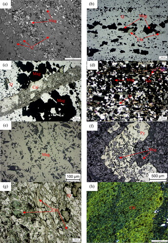
The high-grade iron ore approximately accounts for ca.11.5Mt iron ore reserves, and the largest proven ore body lies in transverse fault of Xishilazi (Figure 2). The high-grade iron ore are mainly composed of magnetite (Figure 3 (e)), with minor quartz, pyrite and chlorite (Figure 3 (f)). They are considered to be resulted from late-stage hypogene hydrothermal enrichment by reactivation and reprecipitation of iron in BIF protore, weather along the strike-slip fault or transverse fault.

The immediate wall rocks of BIF ore in Qidashan Iron District is low grade metamorphic rocks of Neoarchean Yingtaoyuan formation. The lithology is mainly chloritic quartz schist where chlorite is often pale-green (Figure 3 (g)). However, wherever the high-grade iron ore occurs, there must be strong chloritization in wall rocks (Figure 3 (h)) (Zhou 1994; Li H, Yang, et al. 2015). In this case, the chlorites are usually dark-green, suggestive of a relatively high iron content.

3. Data and methods

3.1. Data sources

3.1.1. ZY1-02D data

China ZY1-02D satellite hyperspectral spectrometer was launched in September 2019, and it is well-known for its wide coverage, excellent SNR, full wavelength range and fine spectral resolution (Liu et al. 2020). The hyperspectral image has 166 bands ranging from 400 to 2500 nm, among which 76 bands are in visible to near-infrared range (395-1040 nm) with 10 nm spectral resolution, and 90 bands in short-wave infrared range (1005-2501 nm) with 20 nm spectral resolution. The spatial resolution is 30 m with 60 km swath width, indicating that it can continuously provide detailed spectral information of ground targets (Lu et al. 2021). ZY1-02D hyperspectral images have been successfully applied to geological mapping and mineral exploration (Li et al. 2020). The specific parameters of the hyperspectral spectrometer are list in Table 1.

Table 1. List of parameters of ZY1-02D spectrometer.

Name	Parameter
orbit	Sun synchronous
wavelength /nm	VNIR:395-1040 SWIR:1005-2501
Spatial Resolution /m	30
Spectral Resolution /nm	VNIR:10; SWIR:20
Number of bands	166
Swath width /km	60
Average orbital height /km	778
Side swing ability / degree	±26
Recurrent /day	3
Global coverage capacity/ day	55
Number of bits /bit	12

The data used in this article is the L1A level preprocessing satellite image, with central coordinate 123.02° E and 41.04° N. The image was collected in October 2020, and the whole image is cloudless with excellent contrast of ground objects.

3.1.2. Point spectral measurement by ASD spectrometer

Bulk samples were rinsed with a soft brush, and air-dried for at least 72h. The reflectance spectra were taken by ASD FieldSpec-3 spectrometer with a contact probe of 20 mm in diameter. The instrument has three detectors with the full spectral wavelength range from 350 to 2500 nm. The spectral resolution (channel width) is 3 nm in the VNIR (300-1000 nm), and 10 nm in the SWIR (1000-2500 nm). The spectral radiance over a standardized white spectralon was measured 20 times respectively and their mean value was calculated and recorded as the final spectrum of an individual measurement.

3.1.3. Close range hyperspectral images by HySpex-320m spectrometer

The selected four rock samples, including two altered rock samples peripheral to high-grade iron ore and two chloritic schist wall-rock specimens, were sliced, and the hyperspectral images were taken by HySpex-320m imaging spectrometer in Planetary Mineralogy and Spectroscopy Laboratory, University of Hong Kong. The spectrometer is 0.5 m above the rock slices during imaging, resulting in the fine spatial resolution of ca.0.3 mm. The distinct spectral parameters of the three different hyperspectral spectrometers are listed in Table 2.

Table 2. List of spectral parameters of ASD, HySpex and ZY1-02D spectrometers.

Name	ASD	HySpex	ZY1-02D
Wavelength /nm	VNIR:350 ∼ 1000	VNIR:400 ∼ 1000	VNIR:395-1040
	SWIR: 1000 ∼ 2500	SWIR: 1000 ∼ 2500	SWIR:1005-2501
Spectral Resolution /nm	VNIR: 3.0	VNIR: 3.70	VNIR:10
	SWIR: 10.0	SWIR: 6.30	SWIR:20
Spatial Resolution /m	Circular (diameter0.02)	0.0003	30
Distance between sensor and target /m	0 (contact probe)	0.5	778000

3.1.4 X-ray diffraction (XRD)

Mineral compositions of selected iron ore and wall rock samples were analysed by SmartLab intelligent X-ray diffractometer of Rigaku Ltd., Japan, at Northeastern University, Shenyang, P.R. China. The system is fitted with a Cu cube. The samples were grinded into 200 mesh powder and prepared as random powder. The operating conditions were 45KV accelerating voltage and 200 mA accelerating current, and the testing range is 5-90°. The data were processed by Jade 6.0 software, and smoothed, plotted and labelled in Origin software package.

3.2. Methods

3.2.1. Data preprocessing

The data processing methods of ASD point measurements and HySpex hyperspectral images can be seen from Hao et al. (Hao et al. 2020) for detail. So only the data processing of ZY1-02D is discussed below.

The preprocessing of remote sensing data is to reduce the influence of atmosphere, topography and imaging conditions, etc., so as to reconstruct the reflectance spectrum of the ground targets. All the processing was done by ENVI 4.7 software, including:

1. Removal of overlapping bands: There is overlapping bands between VNIR (395- 1040 nm) and SWIR (1005-2501 nm), so the redundant bands should be removed.

2. Radiation calibration: The L1A digital product of the ZY1-02D satellite (DN value) was converted into radiance value.

3. Destriping: Vertical striping errors are common for most pushbroom imaging systems (Han et al. 2002), especially the low frequency SWIR spectral bands (Goodenough et al. 2003), so is the case of ZY1-02D hyperspectral data. In this article, Fourier Transform method was used to reduce the periodical noise.

4. Atmospheric correction: Atmospheric correction is essential to the hyperspectral image processing. The FLAASH (Fast Line-of-Sight Atmospheric Analysis of Spectral Hypercubes) atmospheric correction module in ENVI 4.7 was adopted to correct the ZY02D image. After atmospheric correction, the water vapour absorption bands (1341-1425 nm and 1812-1946 nm, respectively) were removed due to the effect of atmospheric water (Figure 4).

5. The Savitzky–Golay (S-G) filtering: S-G smoothing is intrinsically a sliding window least squares filtering, and commonly used in hyperspectral data processing due to the consideration of retaining the spectral characteristics as much as possible (Savitzky and Golay 1964; Ruffin et al. 2008).

6. Continuum-removal: In reflectance spectroscopy, the continuum is considered to be ‘background’ and should be removed prior to further characterization of the spectral absorption features in hyperspectral images (Clark and Roush 1984; Clark et al. 1990; Clark 1999; Hecker, van Ruitenbeek, van der Werff, et al. 2019). In this article, SNR of ZY1-02D hyperspectral data in Archean ‘dark’ BIF ore district is relatively low, no satisfactory results can be obtained by full range continuum removal method, thus only the hull from SWIR range were removed.

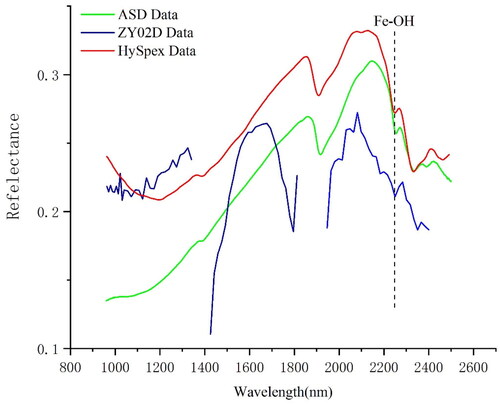
Figure 4. Spectra of ASD, HySpex and ZY1-02D after preprocessing.

3.2.2. Determination of Fe-OH absorption feature of chlorite

The within-species variability of chlorite is marked by the spectral features at 2250 and 2350 nm (Hunt 1977; Clark 1999; Cloutier et al. 2021), which has long been regarded as an excellent indicator to the metallogeny and mineral prospecting (Thompson et al. 1999; Meijering and Falk 2002; Lin and Sun 2015; Cloutier et al. 2021; Hao 2021). Considering that both sericite and carbonate minerals in BIF ore also manifest obvious absorption features near 2350 nm, only the Fe-OH absorption band at ca.2250 nm is selected for the compositional mapping of chlorites in this article. Generally speaking, the Mg-rich chlorite exhibits Fe-OH absorption between 2240 and 2249 nm, intermediate (or Mg-Fe) chlorite varies between 2250 and 2255 nm, and the Fe-rich between 2256 and 2265 nm (Cloutier et al. 2021). Therefore, accurate determination of the diagnostic absorption wavelength is of great importance to the identification of within-species variability of chlorites.

The absorption feature was determined by 1^st derivative method. Taking the band near 2250 or 2267 nm as the central band, the 1^st derivative of the reflectance spectral curve composed of three or five consecutive bands was calculated. If the derivative value changes from negative to positive, it means that there is an absorption feature at the central wavelength position.

3.2.3. Wavelength mapping algorithm

The spectral resolution in SWIR range of ZY1-02D is ca.20 nm, which is obviously less fine than that of ASD or HySpex-320m spectrometer (Figure 5). This means the two kinds of chlorites, which can easily be discriminated by the latter two methods, perhaps cannot be distinguished by ZY1-02D data. Furthermore, the wavelength threshold value used for the discrimination of the two kinds of chlorites probably don’t lies exactly on the specific band. Appropriate and valid wavelength mapping is the key to resolve this problem.

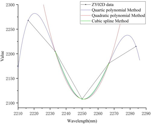
Figure 5. Interpolated curves by quadratic polynomial, cubic spline and quartic polynomial method.

1. Quadratic polynomial method

   Quadratic method is proven to be a simple, accurate and instrument-independent method for estimating the wavelength positions of absorption features and widely used for non-imaging hyperspectral data and a variety of imaging hyperspectral instruments, such as PIMA, AVIRIS, HyMap and others with different sampling intervals and SNRs (Kruse 1988; Rodger et al. 2012; van Ruitenbeek et al. 2014; van der Meer et al. 2018; Hecker, van Ruitenbeek, Bakker, et al. 2019). In this case, three band values are enough for the solution of the problem. Taking the selected three bands, i.e., the band with deepest absorption features, and the bands before and after this band, a quadratic polynomial function is calculated using Equations (1)(1) $${\omega }_2\left(\mathrm{x}\right)={\mathrm{ax}}^2+\mathrm{bx}+\mathrm{c}$$(1) and (2)(2) $$x_{2min}=-\frac{\mathrm{b}}{2\mathrm{a}}$$(2) . (1) $${\omega }_2\left(\mathrm{x}\right)={\mathrm{ax}}^2+\mathrm{bx}+\mathrm{c}$$(1)

   where ${\mathrm{\omega }}_2\left(\mathrm{x}\right)$ is the estimated reflectivity at wavelength position x; a, b and c are the coefficients of the function. (2) $$x_{2min}=-\frac{\mathrm{b}}{2\mathrm{a}}$$(2)

   $x_{2min}$ is the interpolated wavelength position at minimum reflectance; a and b are the coefficients of the function.

2. Quartic polynomial method

   Another method popularly used for wavelength mapping is quartic polynomial method (McCord et al. 1981; Tan and Md Ali 2013), which at least five band values are needed. The detailed function of quartic polynomial method is as Equation (3)(3) $${\mathrm{\omega }}_4\left(\mathrm{x}\right)=\mathrm{a}{\mathrm{x}}^4+\mathrm{b}{\mathrm{x}}^3+\mathrm{c}{\mathrm{x}}^2+\mathrm{dx}+\mathrm{e}$$(3) : (3) $${\mathrm{\omega }}_4\left(\mathrm{x}\right)=\mathrm{a}{\mathrm{x}}^4+\mathrm{b}{\mathrm{x}}^3+\mathrm{c}{\mathrm{x}}^2+\mathrm{dx}+\mathrm{e}$$(3)

   where ${\mathrm{\omega }}_4\left(\mathrm{x}\right)$ is the estimated reflectivity at wavelength position x, and a, b, c, d and e are the coefficients of this function.

   If the 1^st derivative of ${\mathrm{\omega }}_4\left(\mathrm{x}\right)$ is 0, it means the spectrum is at the wavelength where spectral summit or trough locates. In this article, the minimum value near 2250 using Equations (4)(4) $${\omega }_4^{\prime }\left(x\right)=4a{x}^3+3b{x}^2+2cx+d$$(4) and (5)(5) $${\omega }_4^{″}\left(x\right)=12a{x}^2+6bx+2c$$(5) : (4) $${\omega }_4^{\prime }\left(x\right)=4a{x}^3+3b{x}^2+2cx+d$$(4) (5) $${\omega }_4^{″}\left(x\right)=12a{x}^2+6bx+2c$$(5)

   When ${\mathrm{\omega }}_4^{\prime }({\mathrm{x}}_i)$=0 and ${\mathrm{\omega }}_4^{″}\left({\mathrm{x}}_i\right)$>0 (i = 1, 2, 3), the corresponding $x_i$ is the deepest absorption wavelength position.

3. Cubic spline method

   Cubic spline method is commonly used in the field of curve smoothing, and of course it can also be used to interpolate the wavelength position and estimate the depth of the absorption features of hyperspectral data (Clark 1980; Goodenough et al. 2003; Tong et al. 2006). The interpolation by cubic spine method requires the function to be second order differential. The following conditions should be satisfied:

4. On each piecewise interval [$x_i,$ $\mathrm{ }{x}_{i+1}$], ${\mathrm{\omega }}_3\left(\mathrm{x}\right)$ is a cubic equation;

5. Interpolation conditions, ${\mathrm{\omega }}_3\left({\mathrm{x}}_i\right)=y_i(i=0,1,\dots ,n);$

6. The curve is smooth, i.e., ${\mathrm{\omega }}_3\left(\mathrm{x}\right),$ ${\omega }_3^{\prime }\left(\mathrm{x}\right)$ and ${\omega }_3^{″}\left(\mathrm{x}\right)$ are continuous;

7. Natural boundary, ${\mathrm{\omega }}_3^{″}\left({\mathrm{x}}_0\right)={\mathrm{\omega }}_3^{″}\left({\mathrm{x}}_{\mathrm{n}}\right)=0;$

   According to the conditions mentioned above, the equation can be rewritten as Equation (6)(6) $${\omega }_3\left(x\right)=a{x}^3+b{x}^2+cx+d$$(6) . (6) $${\omega }_3\left(x\right)=a{x}^3+b{x}^2+cx+d$$(6)

4. Results

4.1. Results of wavelength mapping

The deepest absorption band between 2233 and 2267 nm was determined by 1^st derivative method. The values of three consecutive bands are enough for the calculation of quadratic polynomial and cubic spline method, whereas at least five values are needed for quartic polynomial method. The results of interpolated wavelength are illustrated in (Table 3, Figures 6 and 7).

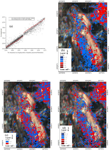
Figure 6. Raw wavelength positions (horizontal coordinate) and interpolated wavelength positions (longitudinal coordinate); (a) quadratic polynomial; (b) cubic spline; (c) quartic polynomial.

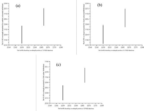
Figure 7. Spatial distribution of interpolated wavelength positions in the Qidashan open-pit iron district (a) quadratic polynomial; (b) cubic spline; (c) quartic polynomial method.

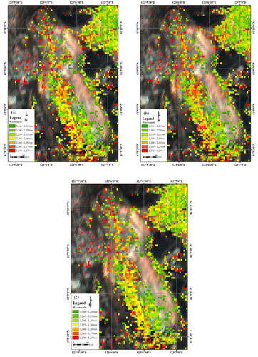
Table 3. Statistics of the wavelength mapping by quadratic polynomial, cubic spline and quartic polynomial method.

Method	Before interpolation	After interpolation
		Max	Min	Median	Mode	Average	MSE
Quadratic polynomial	2250	2258.32	2241.69	2251.11	2254.00	2250.79	4.40
	2267	2275.09	2258.60	2266.36	2264.00	2266.54	4.49
Cubic spline	2250	2256.96	2242.96	2250.66	2249.00	2250.56	3.43
	2267	2273.70	2259.90	2266.50	2266.00	2266.56	3.49
Quartic polynomial	2250	2259.24	2239.48	2251.20	2251.00	2250.92	3.97
	2267	2274.72	2257.33	2264.49	2263.00	2265.02	4.29

The results indicate that the wavelength positions interpolated by the three methods are similar, i.e. all the interpolated values are stretched to the full range between 2240 and 2275 nm (Table 3), which are theoretically more suitable for the identification of the within-species variability of chlorites. The minimum values of quadratic polynomial, cubic spline and quadric polynomial method are 2241.69, 2242.96 and 2239.48, and maximum values 2275.09, 2273.70 and 2274.72 respectively. Notes that the values interpolated by both quadratic and quartic polynomial methods are continuous, and there are even overlapping values by quartic method; However the values interpolated by cubic spline method exhibit obvious non-data interval between band at 2250 and 2267 nm (Figure 6).

The overall spatial distribution of the interpolated wavelength positions (Figure 7) by three methods is also similar, except that the amount of higher values by quartic method is relatively small, especially in the middle part of open-pit and tailing pond near Xishilazi fault, and southernmost part Qidashan open-pit. Detailed image analysis and In-situ investigation show that the southern part was in shadow area during imaging, which probably indicates that the quartic polynomial method is more sensitive to the low SNR targets (shadow area).

4.2. Mineral composition of iron ore and wall rocks, and the types of chlorites by XRD

8 samples, i.e. 2 BIF ore, 2 high grade iron ore, 2 chloritic quartz schist and 2 chloritization rock samples were taken for XRD analysis. The result indicates that the mineral compositions of BIF and high grade iron ore are relatively simple. BIF is mainly composed of quartz and magnetite (Figure 8 (a) and (b)). Note that the minor chlorite observed under microscopy was too low to be detected by XRD. The high grade iron ore chiefly consists of magnetite, with minor quartz, chlorite, and pyrite (Figure 8 (c) and (d)).

Figure 8. XRD Patterns for selected BIF ore (a and b), high grade magnetite ore (c and d), wall rock (e and f), and hydrothermal alteration rock (g and h). Note that the different diffraction peaks of various chlorites between 31.65° and 66.12°, meaning that the chlorites from alteration rocks tend to be of Fe-chlorite type.

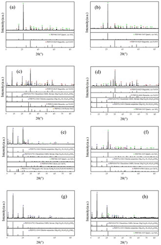
The immediate wall rock of BIF ore is chlorite quartz schist, and mainly composed of chlorite and quartz, with small amount of cacite and phlogopite (Figure 8 (e) and (f)). The major minerals constituting the strong chloritic alteration rocks peripheral to high grade magnetite ore are chlorite, with minor quartz (Figure 8 (g) and (h)). Pay attention to the difference between Powder Diffraction Files of the two kinds of chlorites, as illustrated in the bottom of Figure 8 (e)–(h). In comparison to the chlorite occurred in quartz chlorite schist, the chlorite from alteration rocks exhibits much more diffraction peaks between 31.65° and 66.12°, indicating that the epigenetic hydrothermal chlorite tends to be of Fe-chlorite type, which was consistent with the previous EMPA results (Hao et al. 2020; Hao 2021).

4.3. Identification of two kinds of chlorites by interpolated wavelength mapping

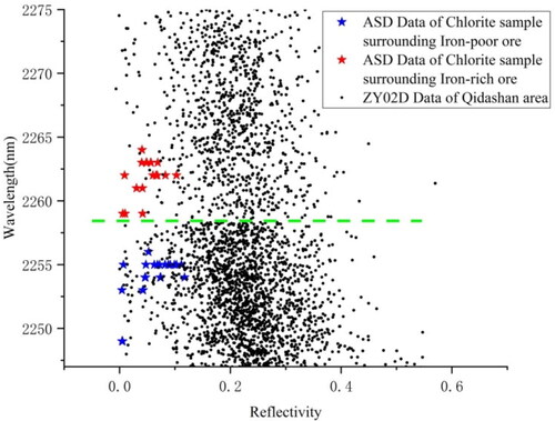
The ASD spectra and close-range HySpex imaging data (Hao et al. 2020) are statistically analysed to determine a suitable threshold value of spectral wavelength for the discrimination of the two kinds of chlorites (Figure 9). Figure 9 (a) indicates that the wavelength values of these two kinds of chlorites slightly overlap between 2250 and 2260 nm, while the box-whisker plot shows that the majority of the wavelength positions are distinctly different (Figure 9 (b)). In consideration of the scatter diagram and the box-whisker statistics of ASD and HySpex spectral data, combined with the scatter map of interpolated Fe-OH wavelength vs. reflectivity of ZY1-02D hyperspectral data (Figure 10), 2258 nm is determined as the final threshold wavelength for the identification of the two kinds of chlorites.

Figure 9. Determination of the threshold value of Fe-OH wavelength position used for the identification of two kinds of chlorites. (a) Scatter map of Fe-OH wavelength by ASD spectra and randomly extracted HySpex data; (b) Box- whisker plot of randomly extracted HySpex data of the two kinds of chlorites in Qidashan Iron Mine.

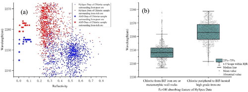
Figure 10. Scatter map of Fe-OH wavelength position vs reflectivity of chlorites by ASD spectra and interpolated ZY1-02D hyperspectral data.

4.4. Spatial distribution of interpolated Fe-OH wavelength of chlorites

According to the wavelength threshold value determined above, the chlorites occurred in Qidashan mining district are classified, and necessary post-classification processing was done to reduce ‘salt and pepper noise’ effect (Figure 11).

Figure 11. Spatial distribution map of two kinds of chlorites. (a) Wavelength interpolated by quadratic polynomial method; (b) wavelength interpolated by cubic spline method; (c) wavelength interpolated by quartic polynomial wavelength; (d) mineral discrimination by reduction of ‘pepper and salt’ effect of (a).

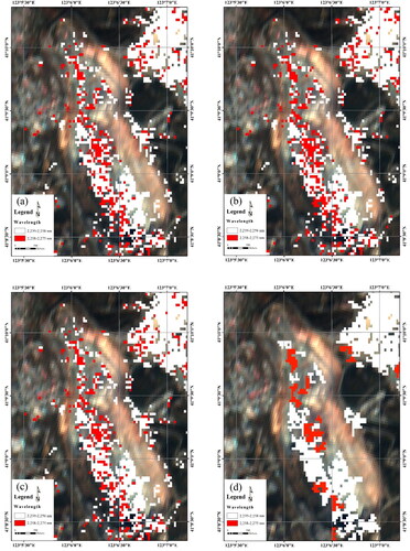
In general, the shape and spatial distribution of the Fe-OH wavelength interpolated by the three methods are similar. The domains with longer Fe-OH wavelength mainly distribute near the transverse fault of Xishilazi and strike-slip fault of Beiershan, which is spatially well in coincidence with the proven high-grade iron ore bodies (Figure 2). This means that the wavelength mapping methods are suitable for the identification of within-species variability of the low-SNR ‘dark’ chlorite.

5. Discussion

5.1. Comparison of the wavelength mapping by the three methods

Spectral wavelength is sensitive to the mineralogy and chemistry of the minerals and rocks under investigation (Clark et al. 1990; Clark 1999; Thompson et al. 1999; van Ruitenbeek et al. 2014; van der Meer et al. 2018; Hecker, van Ruitenbeek, Bakker, et al. 2019; Hecker, van Ruitenbeek, van der Werff, et al. 2019), many scholars have made so much efforts that several specific freeware tools had been programmed (van der Meer et al. 2018; Hecker, van Ruitenbeek, van der Werff, et al. 2019); however, the application is limited by the spectral resolution of most hyperspectral data, especially the relatively low-frequency range of space borne hyperspectral images. In this article, three interpolation methods were applied to map the wavelength positions of ‘dark’ chloritic rocks by China ZY1-02D hyperspectral image. All the three methods give excellent results however small differences still exist.

As mentioned above, the wavelength positions interpolated by quadratic polynomial method are continuous, wide-ranged with no non-data interval or overlapping between the consecutive bands. In this sense, quadratic polynomial method is most suitable for the wavelength mapping of hyperspectral data, and truly it is the most commonly used algorithm for the interpolation of wavelength position (Kruse 1988; Rodger et al. 2012; van Ruitenbeek et al. 2014; van der Meer et al. 2018; Hecker, van Ruitenbeek, Bakker, et al. 2019), therefore the result of quadratic polynomial method is taken as the basis for comparison in the following sections of the article.

Overall the wavelength positions interpolated by quadratic polynomial and quartic polynomial method manifests as a well-defined linear relationship (Figure 12 (a)), i.e. the values and the range of wavelength positions are approximately the same (Figures 6 (a) and (c) 7 (a) and (c)). Nevertheless, they are not strictly linear, especially the outlier values of the lower left and upper right part of the diagonal straight line in Figure 12 (a), which indicates that in the longer wavelength range, the quartic polynomial interpolated values are smaller compared to those interpolated by quadratic polynomial method, and vice versa. As we all know, with the increasing of the order of interpolation polynomials, serious oscillation phenomena will appear, which will increase the computational error and affect the stability of computation, i.e. the ‘Runge Phenomenon’ (Lin and Sun 2015). Interpolation by quartic polynomial method requires two more band values than quadratic polynomial method. In consideration that the spectral resolution of ZY1-02D hyperspectral images is ca.20 nm, the interpolation by quartic polynomial method probably involves the spectral band of Al-OH at 2200 nm or Mg-OH/CO₃^2- band at 2340 nm, which probably explains the outlier values in Figure 12 (a). Although most of the D-values are between quartic and quadratic polynomial ranges from −2 to 2, the difference ranges between −14 and 10 (Figure 12 (b)), therefore other higher order polynomial method is not suggested.

Figure 12. The differences of the interpolated Fe-OH wavelength positions by quadratic polynomial, cubic spline and quartic polynomial method. (a) Scatter map of interpolated wavelength positions among the three methods; (b) Spatial distribution of the D-values between wavelength interpolated by quartic polynomial and quadratic polynomial method; (c) Spatial distribution of the D-values between wavelength interpolated by cubic spline and quadratic polynomial method; (d) Spatial distribution of the D-values between wavelength interpolated by quartic polynomial and cubic spline method.

The cubic spline interpolation method is intrinsically a piecewise third order polynomial interpolation (Meijering and Falk 2002). In most cases, only three band values are involved for the computation of cubic spline interpolation method, which is similar to that of quadratic polynomial method, consequently the results by these two methods are virtually identical, with majority of the D-values between −2 and 2 (Figure 12 (c)), this indirectly validates the conclusion to some degree (Figure 12 (d)). However, the wavelength range interpolated by cubic spline method is about 2-3 nm smaller compared to those of the other two methods (Table 3, Figures 6 and 11(a)), meanwhile with a 3-nm non-data gap between the consecutive bands, which results from the natural boundary conditions of cubic spline method. From this point of view, the wavelength positions interpolated by cubic spline method cannot cover the entire wavelength range, and theoretically is not as practical as the other two methods.

There are little differences among the wavelength mapping results interpolated by the three methods. The reason is that the threshold value determined for the discrimination of the two kinds of chlorites in Qidashan mining district, i.e. 2258 nm, coincidentally lies in the middle of two consecutive bands and happen to be in the non-data interval of cubic spline method. It can be speculated that another threshold value will result in different situation.

In summary, quadratic polynomial method is most suitable for the interpolation of the SWIR wavelength mapping.

5.2. Spatial relationship between the interpolated longer Fe-OH wavelength and BIF-hosted high-grade iron ore in Qidashan Iron Mine

Figure 11 (d) illustrates that the domains with longer wavelength positions interpolated by quadratic polynomial method concentrate in Beiershan strike-slip fault and both sides of Xishilazi transverse fault, which is spatially in well accordance with the BIF-hosted high-grade iron ore in Qidashan Iron Mine (Figures 2 and 13(b) and (c)). A pronounced scenario is that the domain with longer interpolated wavelength in the middle part of No.3 mining sub-district is larger and wider compared to the discovered high grade iron ore bodies.

Figure 13. Field Photographs of Qidashan Iron Mine. (a) High resolution Google image of Qidashan Iron Mine; (b) Field photograph of Beiershan high grade magnetite ore body; (c) Field photograph of high grade magnetite ore body along Xishilazi transverse fault; (d) Field photograph of high grade magnetite ore body in No.3 mining sub-district, where the high magnetic anomaly exists (Figure 14); (e) The relatively high grade iron ore body in lower left corner of the Qidashan open pit.

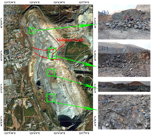
Figure 14. Overlapping map of magnetic survey and the ZY1-02D image in Qidashan open pit.

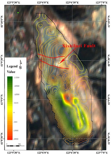
Early in 2014, a ground-based high resolution magnetic survey was carried out in Qidashan open pit mine. The result showed that there was a local higher positive magnetic anomaly in the middle part of No.3 mining sub-area (Wang H et al. 2014). It is fascinating that the domain with higher magnetic anomaly lies immediately south to the longer interpolated wavelength region. Recent development and exploitation works in Qidashan Iron Mine indicate that there are truly high-grade iron ores in deep part where the higher magnetic anomaly exist (Figure 13 (d)). Furthermore, the other anomaly in the lower left corner spatially coincides with another relatively high grade iron ore body (Figure 13 (e)), suggestive of the potential application of wavelength mapping by quadratic polynomial interpolation in exploration of BIF-hosted high-grade iron ore in Anshan area.

5.3. Application of satellite hyperspectral data in evaluation of resource potential in Archean greenstone belts in Eastern Liaoning Province

The Archean metamorphic rocks widely spread in Liaoning Province, among which Anshan group mainly locates in eastern Liaoning Province. The lower part of Anshan group with granulite facies mainly lies in Xinbin and Fushun area, the middle part with amphibolite facies concentrates in Benxi and Liaoyang area, and the upper part localizes in Anshan area (LBOGAMR 1989). All the Archean metamorphic rocks with BIF iron ore enclaves occur as xenoliths in ancient granitic rocks (Zhou 1994). In most of the BIF iron deposit, there exist BIF-hosted high-grade iron bodies with various scale, which are related to the hypogenic hydrothermal fluids and characterized by strong chloritization in wall rocks. The distinctly longer Fe-OH wavelength features of hydrothermal metasomatic chlorites make the exploration of high-grade iron ore by hyperspectral remote sensing technique feasible, fast and less expensive.

In contrast with the ground-based spectrometers and/or close-range hyperspectral imaging system, China ZY1-02D hyperspectral sensor is about 778 km away from the earth’s surface with 30 m spatial resolution. The hyperspectral image used in this article was collected in October, meaning that the solar zenith angle was relatively low during imaging, and part of the Qidashan open pit was in shadow. Furthermore, the studying target is ‘dark’ BIF and chlorite with low SNR. In this sense, the ZY1-02D hyperspectral sensor allows detailed mineral chemistry discrimination by wavelength mapping in such less-than-optimum conditions, demonstrating the pronounced potential in mineral exploration of BIF-hosted high grade iron ore in eastern Liaoning Province.

Recently, it was discovered that there occurred Nb-Ta mineralization in the chloritic alteration rocks proximal to the BIF-hosted high-grade iron ore in eastern Liaoning Province (LBOGAMR 1989). The hyperspectral remote sensing technique is expected to play significant role in the exploration of rare metal resources.

6. Conclusions

1. The subordinate amount of high grade iron ores in China are mainly composed of magnetite, whose ‘flat and featureless’ spectrum makes it difficult to discriminate by reflectance spectroscopy. However, the coeval chlorite in altered wall rocks exhibits prominent longer Fe-OH absorption wavelength, providing an alternative tool for the exploration of BIF-hosted high grade iron ore in eastern Liaoning Province.

2. Quadratic polynomial, cubic spline and quartic polynomial method are adopted to interpolate the Fe-OH wavelength of chlorite by China ZY1-02D hyperspectral data, the result indicates that all the three methods are effective, among which quadratic polynomial method is most suitable for the detailed mapping of within-species variability of chlorite, even though under the less-than-optimum imaging conditions.

3. Recently, it is discovered that there occurred Nb-Ta mineralization in the chloritization altered wall rocks, therefore the space borne hyperspectral remote sensing technique is expected to play significant role in the exploration of BIF-hosted high grade iron ore and the related rare metal mineralization potential in altered wall rocks in eastern Liaoning Province.

Author contributions

Writing- part of original draft preparation, review and editing, Y. Yao; writing- part of original draft preparation and data processing- Z. Li; ASD spectral measurement- J. Liu and T. Hou; field investigation and mineral identification- J. Fu and Y. Zhang; All authors have read and agreed the published version of the manuscript.

Acknowledgements

We thank DiMap for access to the HySpex instruments used in the PSML. The authors were also deeply indebted to Yong-zeng Wang, the chief engineer, and the other colleagues of Qidashan Iron Mine for their kind help in field investigation, magnetic survey and sampling.

Disclosure statement

No potential competing interest was reported by the authors.

Data availability statement

The data that support the findings of this study are available from the corresponding author, [author initials], upon reasonable request.

Additional information

Funding

This work was supported by [the National Key Research and Development Program of China] under Grant [No. 2022YFC2903701]; [the National Key Research and Development Program of China for Young Scientists] under Grant [No. 2022YFC2905400];

References

- Bao H, Liu S, Wang M, Teng G, Sun G. 2020. Mesoarchean geodynamic regime evidenced from diverse granitoid rocks in the Anshan-Benxi area of the North China Craton. Lithos. 366-367:105574. doi: 10.1016/j.lithos.2020.105574.
- Bishop C, Rivard B, de Souza Filho C, van der Meer F. 2018. Geological remote sensing. Int J Appl Earth Obs Geoinf. 64:267–274. doi: 10.1016/j.jag.2017.08.005.
- Bora S, Kumar S, Yi K, Kim N, Lee TH. 2013. Geochemistry and U–Pb SHRIMP zircon chronology of granitoids and microgranular enclaves from Jhirgadandi Pluton of Mahakoshal Belt, Central India Tectonic Zone, India. J Asian Earth Sci. 70-71:99–114. doi: 10.1016/j.jseaes.2013.03.006.
- Clark RN, King TVV, Klejwa M, Swayze GA, Vergo N. 1990. High spectral resolution reflectance spectroscopy of minerals. J Geophys Res. 95(B8):12653. doi: 10.1029/JB095iB08p12653.
- Clark RN, Roush TL. 1984. Reflectance spectroscopy: quantitative analysis techniques for remote sensing applications. J Geophys Res. 89(B7):6329–6340. doi: 10.1029/JB089iB07p06329.
- Clark RN. 1980. A large-scale interactive one-dimensional array processing system. PASP. 92(546):221. doi: 10.1086/130652.
- Clark RN. 1999. Spectroscopy of rocks and minerals and principles of spectroscopy. Remote Sens Earth Sci. 3:3–58.
- Clout JMF, Simonson BM, et al. 2005. Precambrian iron formations and iron formation-hosted iron ore deposits. In: Hedenquist JW, Thompson JFH, Goldfarb RJ, editors. One hundredth anniversary volume. Littleton (CO): Society of Economic Geologists; p. 643-679.
- Cloutier J, Piercey SJ, Huntington J. 2021. Mineralogy, mineral chemistry and SWIR spectral reflectance of chlorite and white mica. Minerals. 11(5):471. doi: 10.3390/min11050471.
- Fonteneau LC, Martini B, Elsenheimer D. 2019. Hyperspectral imaging of sedimentary iron ores – beyond borders. ASEG Extended Abstr. 2019(1):1–5. doi: 10.1080/22020586.2019.12073201.
- Ganesh BP, Aravindan S, Raja S, Thirunavukkarasu A. 2013. Hyperspectral satellite data (Hyperion) preprocessing—a case study on banded magnetite quartzite in Godumalai Hill, Salem, Tamil Nadu, India. Arab J Geosci. 6(9):3249–3256. doi: 10.1007/s12517-012-0584-8.
- Goodenough DG, Dyk A, Niemann KO, Pearlman JS, Chen H, Han T, Murdoch M, West C. 2003. Processing hyperion and ALI for forest classification. IEEE Trans. Geosci. Remote Sens. 6(41):1321–1331. doi: 10.1109/TGRS.2003.813214.
- Hagemann SG, Angerer T, Duuring P, Rosière CA, Figueiredo e Silva RC, Lobato L, Hensler AS, Walde DHG. 2016. BIF-hosted iron mineral system: a review. Ore Geol Rev. 76:317–359. doi: 10.1016/j.oregeorev.2015.11.004.
- Hagemann SG, Rosière CA, Gutzmer J, Beukes NJ. 2008. Banded iron formation-related high-grade iron ore. Vol. 15, SEG Reviews. Littleton (CO): Society of Economic Geologists; p. 1-4.
- Han T, Goodenough DG, Dyk A, Love J. 2002. Detection and correction of abnormal pixels in hyperion images. In: IEEE International Geoscience Remote Sensing Symposium.
- Hao D, Yao Y, Fu J, Michalski JR, Song K. 2020. The laboratory-based HySpex features of chlorite as the exploration tool for high-grade iron ore in Anshan-Benxi area, Liaoning Province, Northeast China. Appl Sci. 10(21):7444. doi:10.3390/app10217444.
- Hao D. 2021. Research on hyperspectral features of Qidashan high-grade iron deposit in Liaoning Province. Shenyang: Northeastern University.
- Hecker C, van Ruitenbeek FJA, Bakker WH, Fagbohun BJ, Riley D, van der Werff HMA, van der Meer FD. 2019. Mapping the wavelength position of mineral features in hyperspectral thermal infrared data. Int J Appl Earth Obs Geoinf. 79:133–140. doi: 10.1016/j.jag.2019.02.013.
- Hecker C, van Ruitenbeek FJA, van der Werff HMA, Bakker WH, Hewson RD, van der Meer FD. 2019. Spectral absorption feature analysis for finding ore: a tutorial on using the method in geological remote sensing. IEEE Geosci Remote Sens Mag. 7(2):51–71. doi: 10.1109/MGRS.2019.2899193.
- Hunt GR. 1971. Visible and near-infrared spectra of minerals and rocks: III. Oxides and hydro-oxides. Modern Geol. 2:195–205.
- Hunt GR. 1977. Spectral signatures of particulate minerals in the visible and near infrared. Geophysics. 42(3):501–513. doi: 10.1190/1.1440721.
- Hunt GR. 1979. Near‐infrared (1.3–2.4) μm spectra of alteration minerals—potential for use in remote sensing. Geophysics. 44(12):1974–1986. doi: 10.1190/1.1440951.
- Izawa MRM, Cloutis EA, Rhind T, Mertzman SA, Applin DM, Stromberg JM, Sherman DM. 2019. Spectral reflectance properties of magnetites: implications for remote sensing. Icarus. 319:525–539. doi: 10.1016/j.icarus.2018.10.002.
- Krupnik D, Khan S. 2019. Close-range, ground-based hyperspectral imaging for mining applications at various scales: review and case studies. Earth-Sci Rev. 198:102952. doi: 10.1016/j.earscirev.2019.102952.
- Kruse FA, Boardman JW, Huntington JF. 2003. Comparison of airborne hyperspectral data and EO-1 hyperion for mineral mapping. IEEE Trans Geosci Remote Sens. 41(6):1388–1400. doi: 10.1109/TGRS.2003.812908.
- Kruse FA. 1988. Use of airborne imaging spectrometer data to map minerals associated with hydrothermally altered rocks in the northern grapevine mountains, Nevada, and California. Remote Sens Environ. 24(1):31–51. doi: 10.1016/0034-4257(88)90004-1.
- Li H, Li L, Yang X, Cheng Y. 2015. Types and geological characteristics of iron deposits in China. J Asian Earth Sci. 103:2–22. doi: 10.1016/j.jseaes.2014.11.003.
- Li H, Yang X, Li L, Zhang Z, Liu M, Yao T, Chen J. 2015. Desilicification and iron activation–reprecipitation in the high-grade magnetite ores in BIFs of the Anshan-Benxi area, China: evidence from geology, geochemistry and stable isotopic characteristics. J Asian Earth Sci. 113:998–1016. doi: 10.1016/j.jseaes.2015.02.011.
- Li L, Li H, Liu M, Yang X, Meng J. 2016. Timing of deposition and tectonothermal events of banded iron formations in the Anshan–Benxi area, Liaoning Province, China: evidence from SHRIMP U-Pb zircon geochronology of the wall rocks. J Asian Earth Sci. 129:276–293. doi: 10.1016/j.jseaes.2016.08.022.
- Li L, Zi J, Li H, Rasmussen B, Wilde SA, Sheppard S, Ma Y, Meng J, Song Z. 2019. High-grade magnetite mineralization at 1.86 Ga in neoarchean banded iron formations, Gongchangling, China: in situ U-Pb geochronology of metamorphic-hydrothermal zircon and monazite. Econ Geol. 114(6):1159–1175. doi: 10.5382/econgeo.4678.
- Li N, Dong X, Gan F, Yan B. 2020. Application evaluation of ZY-1-02D satellite hyperspectral data in geological survey. Spacecraft Eng. 29(06):186–191.
- Lianning Bureau of Geology and Mineral Resources (LBOGAMR). 1989. Regional geology of Liaoning Province. Beijing: Geology Publishing House of China.
- Lin H, Sun L. 2015. Searching globally optimal parameter sequence for defeating Runge phenomenon by immunity genetic algorithm. Appl Math Comput. 264:85–98. doi: 10.1016/j.amc.2015.04.069.
- Liu D, Wilde SA, Wan Y, Wu J, Zhou H, Dong C, Yin X. 2008. New U-Pb and Hf isotopic data confirm Anshan as the oldest preserved segment of the North China craton. Am J Sci. 308(3):200–231. doi: 10.2475/03.2008.02.
- Liu DY, Nutman AP, Compston W, Wu JS, Shen QH. 1992. Remnants of ≥3800 Ma crust in the Chinese part of the Sino-Korean craton. Geol. 20(4):339–342. doi: 10.1130/0091-7613(1992)020<0339:ROMCIT>2.3.CO;2.
- Liu X, Li J, Liu Y, Li W, Wen Q, Liang C, Chang R. 2017. Kinematics analysis and formation mechanism of Qidashan ductile shear zone, Eastern Anshan, Liaoning Province, NE China. Earth Sci. 42:2129–2145.
- Liu X, Li W, Liu Y, Dai L, Dong H, Li J, Zhao Y. 2019. Archean tectonic pattern and its numerical simulation in Anshan area, eastern Liaoning Province. Acta Petrologica Sinica. 35(4):1071–1084.
- Liu Y, Sun D, Liang J, Zhu H, Liu S, Li X. 2020. Overview of ZY-1-02D satellite AHSI on-orbit performance and stability. Spacecraft Eng. 29(06):93–97.
- Lu H, Qiao D, Li Y, Wu S, Deng L. 2021. Fusion of China ZY-1 02D hyperspectral data and multispectral data: which methods should be used? Remote Sens. 13(12):2354. doi: 10.3390/rs13122354.
- Magendran T, Sanjeevi S. 2013. A study on the potential of satellite image-derived hyperspectral signatures to assess the grades of iron ore deposits. J Geol Soc India. 82(3):227–235. doi: 10.1007/s12594-013-0145-0.
- Magendran T, Sanjeevi S. 2014. Hyperion image analysis and linear spectral unmixing to evaluate the grades of iron ores in parts of Noamundi, Eastern India. Int J Appl Earth Obs Geoinf. 26:413–426. doi: 10.1016/j.jag.2013.09.004.
- McCord TB, Clark RN, Hawke BR, McFadden LA, Owensby PD, Pieters CM, Adams JB. 1981. Moon: near-infrared spectral reflectance, a first good look. J Geophys Res. 86(B11):10883–10892. doi: 10.1029/JB086iB11p10883.
- Meijering E, Falk H. 2002. Prolog to a chronology of interpolation: from ancient astronomy to modern signal and image processing. Proc IEEE. 90(3):317–318. doi: 10.1109/JPROC.2002.993399.
- Murphy RJ, Chlingaryan A, Melkumyan A. 2015. Gaussian processes for estimating wavelength position of the ferric iron crystal field feature at ∼900 nm from hyperspectral imagery acquired in the short-wave infrared (1002–1355 nm). IEEE Trans Geosci Remote Sens. 53(4):1907–1920. doi: 10.1109/TGRS.2014.2350983.
- Murphy RJ, Schneider S, Monteiro ST. 2014. Consistency of measurements of wavelength position from hyperspectral imagery: use of the ferric iron crystal field absorption at ∼900 nm as an indicator of mineralogy. IEEE Trans Geosci Remote Sens. 52(5):2843–2857. doi: 10.1109/TGRS.2013.2266672.
- Panda S, Jain MK, Jeyaseelan AT. 2018. A study and implications on the potential of satellite image spectral to assess the iron ore grades of Noamundi iron deposits area. J Geol Soc India. 91(2):227–231. doi: 10.1007/s12594-018-0840-y.
- Ramanaidou E, Wells M, Lau I, Laukamp C. 2022. Chapter 6 -Characterization of iron ore by visible and infrared reflectance and Raman spectroscopies. In: Lu, L., editor. Iron Ore. 2nd ed. Cambridge(UK): Woodhead Publishing; p. 209–246.
- Rodger A, Laukamp C, Haest M, Cudahy T. 2012. A simple quadratic method of absorption feature wavelength estimation in continuum removed spectra. Remote Sens Environ. 118:273–283. doi: 10.1016/j.rse.2011.11.025.
- Ruffin C, King RL, Younan NH. 2008. A combined derivative spectroscopy and Savitzky-Golay filtering method for the analysis of hyperspectral data. GIsci Remote Sens. 45(1):1–15. doi: 10.2747/1548-1603.45.1.1.
- Salisbury JW, Walter LS, Vergo N. 1989. Availability of a library of infrared (2.1-25.0 μm) mineral spectra. Am Mineral. 74(7-8):938–939.
- Savitzky A, Golay MJE. 1964. Smoothing and differentiation of data by simplified least squares procedures. Anal Chem. 36(8):1627–1639. doi: 10.1021/ac60214a047.
- Song B, Nutman AP, Liu D, Wu J. 1996. 3800 to 2500 Ma crustal evolution in the Anshan area of Liaoning Province, northeastern China. Precambrian Res. 78(1-3):79–94. doi: 10.1016/0301-9268(95)00070-4.
- SrinivasaPerumal P, Shanmugam S, Ganapathi P. 2020. Satellite imagery and spectral matching for improved estimation of calcium carbonate and iron oxide abundance in mine areas. Arabian J Geosci. 13(18):914. doi: 10.1007/s12517-020-05859-w.
- Sun X, Zhu X-Q, Tang H, Zhang Q, Luo T, Han T. 2014. Protolith reconstruction and geochemical study on the wall rocks of Anshan BIFs, Northeast China: implications for the provenance and tectonic setting. J Geochem Explor. 136:65–75. doi: 10.1016/j.gexplo.2013.10.009.
- Tan SH, Md Ali J. 2013. Quartic and quintic polynomial interpolation. In: Proceedings of the 20th National Symposium on 607 Mathematical Sciences; Putrajaya, Malaysia.
- Thompson AJB, Hauff PL, Robitaille AJ. 1999. Alteration mapping in exploration: application of short-wave infrared (SWIR) spectroscopy. SEG Discov. 39:16–27. doi: 10.5382/SEGnews.1999-39.fea.
- Tong Q, Zhang B, Zheng F. 2006. Hyperspectral remote sensing: principal, technique and application. Beijjing:High Education Press of China; p. 46–47.
- van der Meer F, Kopačková V, Koucká L, van der Werff HMA, van Ruitenbeek FJA, Bakker WH. 2018. Wavelength feature mapping as a proxy to mineral chemistry for investigating geologic systems: an example from the Rodalquilar epithermal system. Int J Appl Earth Obs Geoinf. 64:237–248. doi: 10.1016/j.jag.2017.09.008.
- van Ruitenbeek FJA, Bakker WH, van der Werff HMA, Zegers TE, Oosthoek JHP, Omer ZA, Marsh SH, van der Meer FD. 2014. Mapping the wavelength position of deepest absorption features to explore mineral diversity in hyperspectral images. Planet Space Sci. 101:108–117. doi: 10.1016/j.pss.2014.06.009.
- van Ruitenbeek FJA, Debba P, van der Meer FD, Cudahy T, van der Meijde M, Hale M. 2006. Mapping white micas and their absorption wavelengths using hyperspectral band ratios. Remote Sens Environ. 102(3-4):211–222. doi: 10.1016/j.rse.2006.02.012.
- Wang E, Xia J, Fu J, Jia S, Men Y. 2014. Formation mechanism of Gongchangling high-grade magnetite deposit hosted in Archean BIF, Anshan-Benxi area, Northeastern China. Ore Geol Rev. 57:308–321. doi: 10.1016/j.oregeorev.2013.09.013.
- Wang H, Jia S, Zhang J. 2014. Application of high-precision magnetic survey method in exploration of Qidashan iron ore deposit. Metal Mine. 7:118–121.
- Zhang Z, Hou T, Santosh M, Li H, Li J, Zhang Z, Song X, Wang M. 2014. Spatio-temporal distribution and tectonic settings of the major iron deposits in China: an overview. Ore Geol Rev. 57:247–263. doi: 10.1016/j.oregeorev.2013.08.021.
- Zhao G,Wilde SA,Cawood PA,Sun M. 2001. Archean blocks and their boundaries in the North China Craton: lithological, geochemical, structural and P–T path constraints and tectonic evolution. Precambrian Res. 107(1-2):45–73. doi: 10.1016/S0301-9268(00)00154-6.
- Zhao L, Wang C, Zhang M, Chen T, Mo L, Wang P. 2020. Current exploration status and supply-demand situation of iron ore resources in China mainland. Geol Explor. 56(3):9.
- Zheng M, Wu P, You B. 2022. Economic security evaluation and early warning of iron ore resources in China. Geol Bull China. 41(5):836–845.
- Zhou S. 1994. Geology of banded iron ore in Anshan-Benxi area. Beijing: Geological Publishing House.