Global and pyramid convolutional neural network with hybrid attention mechanism for hyperspectral image classification

Abstract

Convolutional neural networks (CNNs) have shown impressive results in the hyperspectral image (HSI) classification. However, they still face certain limitations that can impact their effectiveness. The kernels in standard convolution have fixed spatial sizes and spectral depths, which cannot capture global semantic features from HSI and the existing methods for extracting multiscale information are inadequate. Based on these, we propose a global and pyramid convolutional network with a hybrid attention mechanism (GPHANet) for HSI classification. GPHANet adopts a two-branch architecture to extract both local and global hyperspectral features, leveraging the strengths of each to enhance classification performance. The local branch employs dynamic pyramid convolution, which customizes parameters for convolutional kernels of multiple scales based on the input image. This design enables the model to accurately and comprehensively extract multiscale feature information, capturing subtle variations in the HSI. The global branch utilizes circular convolution with a global receptive field, enabling each position in the convolutional layers to gather information from the entire input space. This allows the model to learn global contextual features, enhancing its understanding of the overall structure and semantics of the HSI. After extracting deep global and local features, we apply a compact hybrid attention mechanism (HAM) to capture long-range dependencies along both spatial and spectral dimensions, resulting in a more discriminative feature representation. On the Pavia University, Salinas, and Hong Hu datasets, the proposed model achieved overall accuracies of 99.22%, 98.74%, and 96.80%, respectively, using limited training samples. These results are much better compared to the state-of-the-art methods.

Keywords:

• Hyperspectral image classification
• global convolution
• multiscale convolution
• neural network
• attention mechanism

1. Introduction

The processing and analysis technology of hyperspectral images (HSI) has received widespread attention since the spatial resolution and spectral dimension resolution of images captured by hyperspectral imaging technology have been continuously improved. Compared with natural images, hyperspectral images contain hundreds of bands of rich spatial structure and spectral information, which can significantly improve the precise classification of objects, so they are widely used in real-world applications, such as intelligent agriculture (Wieme et al. 2022), environmental monitoring (Du et al. 2022), food and security (Khan et al. 2022).

HSI classification is a typical pixel-level classification task. Each pixel in the image needs to determine its category. However, unlike natural images, the spectral dimensions of HSI are extremely high, which causes space and efficiency problems for classification algorithms. In addition, the limited labelled samples also pose serious challenges to classification methods. During the last few decades, the early HSI classification methods applied traditional machine learning algorithms, such as support vector machine (SVM) (Melgani and Bruzzone 2004) and maximum likelihood estimation (MLE) (Jay and Guillaume 2014). In addition, some of the state-of-the-art HSI classification methods, which are mainly based on traditional machine learning have achieved good classification performance, such as morphological profiles (MP) (Kumar and Dikshit 2017) and extended morphological profiles (EMP) (Gu et al. 2016). However, it is easy to fall into a bottleneck when processing complex data. This is because traditional methods are shallow classifiers based on handcrafted features, so they can only extract the shallow feature of hyperspectral images. Comparatively, the deep learning (DL) method can extract more abstract features of HSIs by using deep and hierarchical models and has the advantage of automatic learning, so it is gradually applied in hyperspectral image classification. In HSI classification tasks, typical DL methods can be summarized into the following six categories: including convolutional neural network (CNN) (Ge et al. 2023), vision transformer (ViT) (Hong et al. 2022; Sun et al. 2022), graph neural network (GNN) (Ding et al. 2021), recurrent neural network (RNN) (Hu et al. 2021; Zhou et al. 2022), generative adversarial network (GAN) (Feng et al. 2022), auto-encoder (AE) (Liu Y et al. 2022).

Compared to other deep learning methods, Convolutional Neural Networks (CNNs) exhibit remarkable robustness to rotations, scaling, and translations, making them highly accurate in analysing and processing data features, particularly in the domain of images. Therefore, CNNs stand out in HSI classification tasks. Since the deep convolutional neural networks (Hu et al. 2015) were proposed, the accuracy of pixel prediction in HSI has been significantly improved from different model architectures. Currently, according to the different attributes of the features extracted by CNN for HSIs, it can be divided into three categories, namely, spectral-based CNN, spatial-based CNN, and spatial-spectral-based CNN. The spectral-based CNN stacks 1D convolutional layers on the spectral dimension to continuously extract deep spectral features. However, the spectral bands of HSIs are numerous and contain a lot of redundant information. Some spectral-based CNN specially designed adaptive calibration and selection algorithms for bands to improve the accuracy of classification (Mou and Zhu 2020). Because the spatial dimension of HSI also contains a lot of information, spatial-based CNN methods integrate the convolutional layer of spatial information into the model to improve the classification ability (Xu et al. 2018). Compared with spectral-based CNN, spatial-based CNN pays more attention to spatial information. To reduce the interference of spectral information, the spatial-based CNN usually uses the PCA method to reduce the spectral dimension of HSI and then stacks 2D convolutional layers to extract deep spatial features (Haut et al. 2019; Kang et al. 2019). However, these networks usually need to be designed deep enough to ensure that the model can capture discriminative features to obtain satisfactory performance. To make full use of spatial and spectral information, a series of spatial-spectral-based CNN is proposed for HSI classification. For example, a depth 3D-CNN is proposed to jointly extract spatial and spectral features (Bing et al. 2019). A hybrid model composed of 2D-CNN and 3D-CNN is proposed to reduce model parameters and achieve efficient spatial and spectral feature extraction (Yu et al. 2020). Recently, the attention mechanism helps the model selectively focus on important features and capture contextual information in images, and it is increasingly playing a crucial role in HSI classification. Li et al. (2020) proposed a double-branch dual-attention (DBDA) network to improve the classification performance of HSI with limited training samples. In DBDA, spatial and channel attention mechanisms (Fu et al. 2019) are employed separately in two branches to extract features. Li et al. (2021) proposed a spectral and spatial global context attention (SSGCA) network for HSI Classification, in which two branches adopt global context attention to fully utilize global contextual information. Ghaderizadeh et al. (2022) broke the limitation of single-scale features and proposed a multiscale dual-branch residual spectral-spatial attention network (MDBRSSN), where two branches consist of 3D convolutional layers at different scales to effectively extract multi-scale information. Furthermore, there have been works that combine classical machine learning models with CNNs (Shah et al. 2022), achieving good classification accuracy and interpretability.

Although convolutional neural networks (CNNs) are effective in extracting image features using stacked convolutional layers, they have limitations that affect the performance of hyperspectral image classification. The fixed spatial and depth sizes of standard convolutions are smaller than the input data, resulting in CNNs gathering information only from local receptive fields. This hinders the capture of long-range dependencies and crucial global features necessary for visual tasks (Hou et al. 2020; 2021). Hyperspectral images also pose challenges due to their mixed land-cover classes and inconsistent spatial representations across categories. Some categories have large spatial representations, while others are extremely small. Standard convolutions struggle to extract multiscale information effectively. Existing multiscale convolution operations rely on static convolutional kernels that treat all inputs equally, disregarding the varying contributions of different scales to the classification task.

Based on the observations above, our goal is to improve classification accuracy with small training samples and reduced time costs. We address two key aspects to achieve this. Firstly, we strive to improve the model’s ability to extract relevant features, effectively leveraging the rich information in HSI. Secondly, we aim to enhance the representation capability of features to obtain more discriminative hyperspectral features. Our proposed solution is the global and pyramidal convolutional network with a hybrid attention mechanism (GPHANet), which consists of two branches: the global branch and the local branch. The former was inspired by a circular convolution (Zhang et al. 2022) to effectively learn global contextual features in the entire spatial locations and the spectral dimension of HSI. The latter applies dynamic pyramidal convolution, which can adaptively adjust the parameters of convolutional kernels with different spatial sizes and different channel numbers according to the input image, to achieve more accurate and detailed multiscale feature extraction. After learning deep global and local features, GPHANet incorporates a hybrid attention mechanism (HAM) module to fuse the global and local features. The HAM simultaneously captures cross-channel information and information between spatial locations and spectral dimensions. This mechanism selectively highlights the most important channels, spatial locations, and spectral dimensions, resulting in more distinctive feature representations. The major contributions of this article are as follows.

1. To break the limitation of the local receptive field of standard convolution, we propose a global spatial spectral convolution module (GSSCM). This module performs global convolution operations on the entire horizontal, vertical, and depth dimensions of HSI input, effectively extracting global spatial-spectral features. In addition, this module uses circular padding and sampling methods to overcome the boundary effects caused by zero padding in standard convolution.

2. To fully extract multiscale features, we developed a dynamic pyramid convolution module (DPCM). This module contains three convolutional kernels with different spatial sizes and spectral depths, allowing for capturing different levels of features from HSI inputs. In addition, the module also includes a dynamic routing module that can assign importance weights to convolutional kernels with different scales based on different inputs, achieving more accurate and detailed multi-scale feature extraction.

3. A multi-feature dual-branch deep learning model GPHANet is proposed for hyperspectral image classification. In GPHANet, the joint use of GSSCM and DPCM can simultaneously capture spatial-spectral features with global contextual information and multi-scale local spatial-spectral features, which brings higher accuracy.

4. An improved hybrid attention mechanism module is proposed, which uses a three-branch structure to capture cross-dimensional interactive information and calculate attention weight, and achieve the fusion between global and local features.

2. Materials and methods

2.1. Related work

2.1.1. CNNs

In deep learning, CNNs are one of the most representative network backbones. By stacking a series of convolutional layers, CNNs can learn different types of features. As the depth increases, the captured features become more accurate and reliable. In the CNNs, features can be calculated as $y_i={\sum }_{j\in L(i)}{W}_{i-j}{x}_j,$ where $y_i$ and $x_i$ are the input and output of position $i,$ $W_{i-j}$ is the weight of position $(i-j),$ and $L(i)$ is the local neighborhood of position $i.$ Therefore, the standard convolution can only aggregate spatial and spectral information from the local receptive fields of fixed-size convolutional kernels in HSI. For HSI classification, since the spatial resolution of the input sample is far less than that of the natural image, zero padding is usually used to ensure that the input and output of the convolutional layer are the same sizes. Therefore, simply increasing the size of the convolutional kernel requires applying more zero padding at the edges of the input samples, which can cause boundary effects because information near the edges of the image is mixed with zeros, making the network sensitive to position. Recently, the community has designed separable convolution (Zhang et al. 2021; Nie et al. 2022; Zhao et al. 2022) to overcome this problem. The deformable convolution introduces a novel approach by altering the sampling position of convolutions in the input space, thereby indirectly expanding the receptive field. However, the scattered sampling positions in deformable convolutions may fail to cover the entire input, potentially resulting in the loss of detailed information. Additionally, each parameter of the convolutional kernel in deformable convolutions requires an extra parameter to learn the sampling offset value. The actual sampling position is determined through bilinear interpolation based on the offset value. Consequently, generating the offset position of each sample necessitates additional memory and computation costs.

2.1.2. Attention mechanism

Attention is a mechanism in the brain that selectively processes sensory information, allowing humans to allocate attention and control focus when performing tasks (Niu et al. 2021). Inspired by this phenomenon, attention mechanisms have been applied to HSI classification, allowing models to focus on more valuable spatial and spectral information among the numerous bands in HSI, showing significant potential. Wang et al. (2021) proposed a lightweight multiscale spectral-spatial attention feature fusion network (LMAFN) for HSI classification, which utilizes the efficient channel attention (ECA) module (Wang et al. 2020) to learn the importance of different channels and adaptively adjust the weights. Dong et al. (2022) introduced a self-attention mechanism to construct a spatial attention module and channel attention module to enhance feature representation capability. In addition, Liu H et al. (2022) proposed a central attention network to highlight target pixels and accurately extract spatial information from the surrounding pixels of the target pixels. Hyperspectral images exhibit nearly continuous spectral curves, where each pixel shows strong correlations with the spatial locations and spectral dimensions of its surrounding region. Existing methods for HSI classification often employ separate spatial and spectral attention mechanisms or simply combine them. However, these methods rarely consider the close relationship between spatial locations and spectral dimensions.

2.2. Architecture of the GPHANet

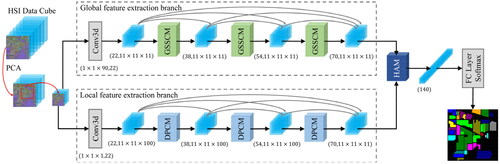
The HSI classification framework based on GPHANet is depicted in Figure 1. We apply PCA to reduce the redundant spectral information in the original HSI data and, at the same time, reduce the computational complexity of the model. GPHANet adopts a dual-branch and densely connected structure similar to DBDA and SSGCA. However, unlike these models that extract spatial and spectral features separately, GPHANet introduces two branches to extract global hyperspectral features and local multiscale hyperspectral features, respectively. In the top branch network, a distinctive global spatial spectral convolution module efficiently captures spatial-spectral features with global context information from the complete spatial locations and spectral dimensions of HSI samples. On the other hand, the bottom branch network employs a pyramid convolution with multiple convolutional kernels of different spatial sizes and spectral depths to comprehensively extract multi-scale spatial-spectral features. Moreover, we incorporate a dynamic routing module into the pyramid convolution to enable the customization of parameters for convolutional kernels at different scales, facilitating precise and detailed multi-scale feature extraction. Subsequently, in the final stages of both branches, a hybrid attention mechanism module is implemented to fuse the extracted global and local multiscale spatial-spectral features while emphasizing the most crucial spatial locations and spectral dimensions for classification. Finally, the fused features are fed into a fully connected (FC) layer to generate prediction results. The loss function used for training the GPHANet model is the cross-entropy loss, defined as follows: (1) $$\mathit{Loss}=-\frac{1}{M}\sum _{m=0}^M\sum _{k=0}^K{y}_k\log \hspace{0.17em}{\widehat{y}}_k+(1-y_k)\log \hspace{0.17em}(1-{\widehat{y}}_k)$$(1) where $K$ represents the number of classes in HSI dataset and $M$ is the size of the mini-batch. $y_k$ and ${\widehat{y}}_k$ represents the true labels and the predicted labels, respectively.

Figure 1. The GPHANet architecture for hyperspectral image classification.

2.3. Global spatial spectral convolution module

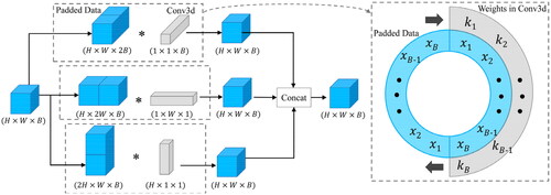
In CNN, a larger receptive field allows neurons to capture a broader range of contextual information, enabling them to capture long-range dependencies and global structures in the input data. Inspired by circular convolution, we build a global spatial spectral convolution module (GSSCM) to overcome the limitation of standard convolutional kernels with limited receptive fields. The convolutional kernels of GSSCM cover the whole spatial locations and spectral dimensions and overcome the defect of zero padding, which can effectively extract the global spatial and spectral information and obtain more powerful feature representations. The details are as follows:

Assuming the input $X$ with dimensions $(H\times W\times B).$ Using a standard 3D convolution with a size of $H\times W\times B$ to extract spatial and spectral information from the entire input space requires a large number of parameters and computational costs, while zero padding can lead to significant boundary effects (Alsallakh et al. 2020; Kayhan and Gemert 2020). Inspired by Inception-v4 (Szegedy et al. 2017), we decompose the standard convolution to achieve flexible and lightweight global spatial spectral feature extraction. As shown in Figure 2, we decompose a 3D convolution with a size of $H\times W\times B$ into three asymmetric global convolutions: global vertical convolution (GVConv) with a size of $H\times 1\times 1,$ global horizontal convolution (GHConv) with a size of $1\times W\times 1$ and global spectral convolution (GSConv) with a size of $1\times 1\times B.$ Compared with single convolution, the multiple global convolutions have stronger feature representation ability and fewer parameters. To overcome the boundary effect caused by zero padding, we perform a circular padding operation to concatenate input $X$ and its copies along the spectral, vertical, and horizontal directions, respectively. Then, we perform circular sampling and global convolution operations throughout the entire input space. Therefore, the information on the edge of the image is no longer convolved with zeros, but with the information on the other side. For standard convolution, even if the size of the convolutional kernel is extended to the whole input space, it can only cover part of the input. Especially for the feature extraction of the image edge, only half of the input covered by the convolutional kernel comes from the original input, while the other pixels are zero. The global spatial-spectral convolution makes our GPHANet more robust and reduces the interference of redundant information caused by zero padding. Given a feature map with a size of $(1,H\times W\times B),$ the output of GVConv at the position $(x,y,z)$ can be calculated with: (2) $${\nu }_{lj}^{\mathit{xyz}}=\sum _m\sum _{h=0}^{H_l-1}{k}_{l,j,m}^h{v}_{\left(l-1\right),m}^{\left(x+h\right)\mathrm{m}\mathrm{od}H,y,z}+d_{l,j}$$(2) where $m$ is the index of the feature map in the $(l-1)$ th layer. Additionally, ${\nu }_{lj}^{\mathit{xyz}}$ represents the output at position $(x,y,z)$ on the $j$ th feature maps of the $l$ th layer. $H$ represents the height dimension of the convolutional kernel. Additionally, $k_{l,j,m}^h$ is the weight at position $h$ of the convolutional kernel corresponding to the $m$ th feature maps, and the $d_{l,j}$ represents the bias. Similarly, given a feature map with a size of $(1,H\times W\times B),$ the output of GHConv at the position $(x,y,z)$ can be calculated with: (3) $${\nu }_{lj}^{\mathit{xyz}}=\sum _m\sum _{w=0}^{W_l-1}{k}_{l,j,m}^w{v}_{\left(l-1\right),m}^{\mathrm{x},\left(y+w\right)\mathrm{m}\mathrm{od}W,z}+d_{l,j}$$(3) where $W$ represents the width dimension of the convolutional kernel. Additionally, $k_{l,j,m}^w$ is the weight at position $w$ of the convolutional kernel corresponding to the $m$ th feature maps. Finally, given a feature map with a size of $(1,H\times W\times B),$ the output of GSConv at the position $(x,y,z)$ can be calculated with: (4) $${\nu }_{lj}^{\mathit{xyz}}=\sum _m\sum _{b=0}^{B_l-1}{k}_{l,j,m}^b{v}_{\left(l-1\right),m}^{\mathrm{x},y,\left(z+b\right)\mathrm{m}\mathrm{od}B}+d_{l,j}$$(4) where $B$ represents the spectral dimension of the convolutional kernel. Additionally, $k_{l,j,m}^b$ is the weight at position $b$ of the convolutional kernel corresponding to the $m$ th feature maps. In addition, rectified linear unit (ReLU) is still widely used by the HSI classification method based on CNN due to its efficiency and simplicity. To better adapt the global receptive fields, GSSCM uses the Gaussian Error Linear Units (GELUs) to improve the expression ability of the model. As a smoothing variant of ReLU, GELU has been used by some of the most advanced transformers and has proven to perform better in capturing long-term dependencies. Assuming that the input is $X,$ the GELU nonlinear activation function can be expressed as: (5) $$\mathit{GELU}\left(X\right)=\frac{X}{2}\times (1+\mathit{erf}\left(\frac{X}{\sqrt{2}}\right))$$(5)

Figure 2. The structure of GSSCM.

Furthermore, Batch Normalization (BN) is utilized in GSSCM to solve the internal covariance shift problem of output activation, which can be defined as: (6) $$BN\left(X\right)=\max \left\{\frac{X-u}{\sqrt{{\sigma }^2+ϵ}}+\gamma ,0\right\}$$(6) where $\gamma$ and $ϵ$ indicates the learnable parameter of scale shift, $u$ and ${\sigma }^2$ represent the mean and variance of the input $X$ respectively.

2.4. Dynamic pyramid convolution module

Although single-scale convolution has a strong local feature extraction ability, the discrimination ability of learned features may be insufficient to challenge the classification (Li et al. 2019) of complex HSI datasets. Duta et al. (2020) proposed pyramid convolution, which consists of multiple types of convolutional kernels with varying spatial resolutions and depths, enabling the effective extraction of multi-scale features. The pyramid convolution also adopts the strategy of group convolution, achieving a similar computational cost to standard convolution. Recently, some works have also adopted the idea of pyramid convolution to process HSI data at multiple scales (Shi et al. 2021; Yang et al. 2022). The currently applied multiscale HSI feature extraction uses a static convolutional kernel to treat all inputs equally. However, different scales of information captured from different input samples also have different contributions to classification.

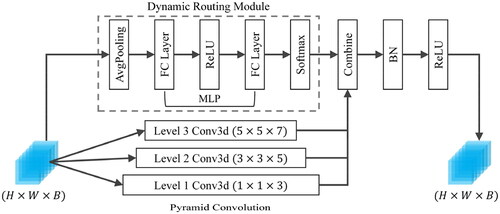
Motivated by this (Chen et al. 2020), we propose a dynamic pyramid convolution module (DPCM) to extract multiscale spatial-spectral features. As shown in Figure 3, DPCM mainly consists of a dynamic routing module and pyramid convolution. Compared with the standard pyramid convolution, DPCM has a dynamic routing module, which can generate the importance weight according to the input and dynamically adjust the parameters of convolutional kernels with different spatial sizes and different channel numbers to achieve more accurate and detailed multiscale feature extraction. Assuming that the input data is $X,$ the output $y$ of DPCM can be regarded as a linear combination of the weights of $k$ convolutional kernels, which can be expressed by the following formula: (7) $$y=\mathit{ReLU}\left({\alpha }_1\left(W_1*X\right)+\dots +{\alpha }_k(W_k*X\right))$$(7) where $W_k$ represents the weight of the $k$ th convolutional kernel, $*$ represents the convolution operation, and $a$ represents the importance weight, which is generated by the dynamic routing module. To ensure the efficiency of DPCM, the dynamic routing module is implemented by the average pooling (AvgPool), multilayer perceptron (MLP), and softmax layer, with their parameters learned during the model training process. Assuming the input $X$ has only one channel and the corresponding shape is $(H\times W\times B),$ the weight ${\alpha }_k$ assigned to the $k$ th convolutional kernel by the dynamic routing module can be expressed as: (8) $$\mathrm{AvgPool}\left(X\right)=\frac{1}{H\times W\times B}\sum _{h=1}^H\sum _{w=1}^W\sum _{b=1}^{B}X\left(h,w,b\right)$$(8) (9) $${\alpha }_k=\frac{\exp \hspace{0.17em}\left({\mathit{MLP}}_i\left(\mathrm{AvgPool}\right(X\left)\right)\right)}{\sum _{k=1}^n\exp \hspace{0.17em}\left({\mathit{MLP}}_i\left(\mathrm{AvgPool}\right(X\left)\right)\right)},\mathrm{ }k=1,\dots ,n$$(9) where $n$ represents the number of convolutional kernels in DPCM, ${\mathit{MLP}}_i$ represents the $i$ th value generated by the input data through MLP.

Figure 3. The structure of DPCM.

2.5. Hybrid attention mechanism module

HSI data contains rich spatial and spectral information, making efficient extraction of distinctive features from HSI crucial for classification performance. Inspired by coordinate attention (Hou et al. 2021), we propose a hybrid attention mechanism module (HAM) to capture cross-dimensional interaction information and calculate attention weights. Compared to attention mechanisms that solely focus on different spatial locations or different channels, the proposed HAM also considers the relationship between spatial locations and spectral dimensions. Each element in the attention map generated by HAM reflects whether the object of interest exists at the corresponding spatial locations and spectral dimensions. This strategy enables HAM to more accurately query the location of the object of interest, thereby assisting the model in better classification.

The detailed implementation of HAM is presented in Figure 4, consisting of three branches. Let $X$ denote the input with dimensions $(C,H,W,B),$ where $C,$ $H,$ $W,$ and $B$ correspond to channel, height, width, and spectral dimensions, respectively. The first branch models the relationship between channel $C$ and spectral dimension $B.$ To obtain richer and more diverse features from HSI and enhance the representation ability of the model, we simultaneously employed max pooling and average pooling to capture two different feature maps $F_B^{\mathrm{Max}}$ and $F_B^{\mathit{Avg}}.$ Then, we utilized two learnable parameters, $a_B$ and ${\beta }_B,$ to adaptively adjust these feature maps and generate enhanced feature map $F_B^E,$ with dimensions $(C,1,1,B).$ This can be expressed as follows: (10) $$F_B^E=a_B{\times F}_B^{\mathrm{Max}}+{\beta }_B{\times F}_B^{\mathit{Avg}}$$(10) where $a_B$ and ${\beta }_B$ are initialized to 0.5 and are automatically learned during the network training process. By introducing these two trainable parameters, more flexible features can be generated between the max pooling and average pooling. The second branch models the relationship between channel $C$ and spatial dimensions $W.$ Similarly, we utilized both max pooling and average pooling to capture two different feature maps $F_W^{\mathrm{Max}}$ and $F_W^{\mathit{Avg}}.$ Two trainable parameters, $a_W$ and ${\beta }_W,$ are used for adaptive adjustment and generating the enhanced feature map $F_W^E,$ with dimensions $(C,1,W,1).$ In the last branch, we focused on the relationship between channel $C$ and spatial dimensions $H.$ We employed both max pooling and average pooling operations to obtain two different feature maps, $F_H^{\mathrm{Max}}$ and $F_H^{\mathit{Avg}}.$ These maps were adaptively adjusted using learnable parameters, $a_H$ and ${\beta }_H,$ resulting in an enhanced feature map $F_H^E,$ with dimensions $(C,H,1,1).$ This process can be summarized by the following equations: (11) $$F_W^E=a_W{\times F}_W^{\mathrm{Max}}+{\beta }_W{\times F}_W^{\mathit{Avg}}$$(11) (12) $$F_H^E=a_H{\times F}_H^{\mathrm{Max}}+{\beta }_H{\times F}_H^{\mathit{Avg}}$$(12) where $a_W,$ ${\beta }_W,$ $a_H$ and ${\beta }_H$ are initialized to 0.5. Next, we concatenate the enhanced feature maps $F_B^E,$ $F_W^E,$ $F_H^E$ and feed them into a shared convolution block to achieve cross-dimensional information interaction between different spatial locations and spectral dimensions. To achieve this goal simple and efficient, the shared convolution block adopts two convolutional layers to form a bottleneck, with a size of $C/r\times 1\times 1\times 1.$ Here, $r$ is the reduction ratio, which works best when set to 5. This can be expressed as follows: (13) $$F_C={\sigma }_2\left(W_2*{\sigma }_1\right(W_1*\left(\mathrm{Concat}\right[F_B^E,F_W^E,F_H^E\left]\right)\left)\right)$$(13) where $\mathrm{Concat}$ denotes the concatenation operation, $\sigma$ is a ReLU activation function. Additionally, $W$ represents the weight of the convolutional kernel, $*$ represents the convolution operation. Next, we divide $F_C$ into three independent features, $F_B,$ $F_W,$ and $F_H,$ along the spectral and spatial dimensions. We then utilize three $C\times 1\times 1\times 1$ convolutional layers to generate the final attention maps $A_B,$ $A_W,$ and $A_H.$ These attention maps indicate the spatial locations and spectral dimensions that contribute the most to the classification, and they can be used to enhance the discriminability of the extracted feature: (14) $$F_O=X\times A_B\times A_W\times A_H$$(14) where $F_O$ represents the final refined feature maps and $X$ represents the input feature maps.

Figure 4. The structure of HAM.

3. Experiments results and analysis

3.1. Datasets

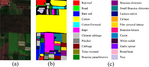
In this article, three real datasets are utilized to evaluate the classification ability of GPHANet. The first is Pavia University (PU) dataset, which contains 610 × 610 pixels, 103 bands, and 9 ground-truth classes. The scene was captured by the reflective optical system imaging spectrometer (ROSIS) optical sensor in Pavia, northern Italy, with a spatial resolution of 1.3 m per pixel. The second is called the Salinas (SA) dataset, which contains 512 × 217 pixels and 200 bands, and 16 ground-truth classes. The scene was captured by the airborne visible infrared imaging spectrometer (AVIRIS) in Salinas Valley, California, USA, with a spatial resolution of 3.7 m per pixel. The last one is the HongHu (HO) dataset, which contains 940 × 475 pixels, 270 bands, and 22 ground-truth classes. The scene was captured by the Headwall Nano-Hyperspec imaging sensor in Honghu City, Hubei Province, China, with a spatial resolution of 0.043 m per pixel. Figures 5–7 shows the false-colour composition and the corresponding ground truth of these three datasets.

Figure 5. False-colour composition and the ground truth of the PU dataset.

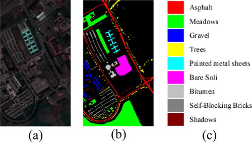
Figure 6. False-colour composition and the ground truth of the SA dataset.

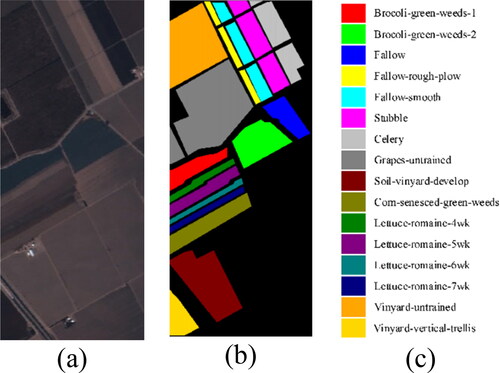
Figure 7. False-colour composition and the ground truth of the HO dataset.

3.2. Experimental settings

The experiment was conducted on a hardware setup consisting of an I7-8750H processor, Nvidia GeForce 1070 MAX-Q GPU, and 16GB RAM. To develop our model, we utilized various software packages, including Python 3.8, PyTorch 1.8, Scikit-learn 1.0, and Cuda 11.1. During the training process, we set the number of epochs to 200 and used a batch size of 32. The initial learning rate of the model was set to 0.0005, and we employed the cosine annealing algorithm to dynamically adjust the learning rate, thereby preventing the model from getting stuck in a local minimum. To assess the classification performance, we employed several quantitative indicators. The average accuracy (AA) represents the proportion of correctly classified samples among the total samples. The overall accuracy (OA) measures the classification accuracy of each class individually. Additionally, we used Kappa coefficients to evaluate the similarity between the classification results and the ground truth.

3.3. Analysis of the influences of different parameters

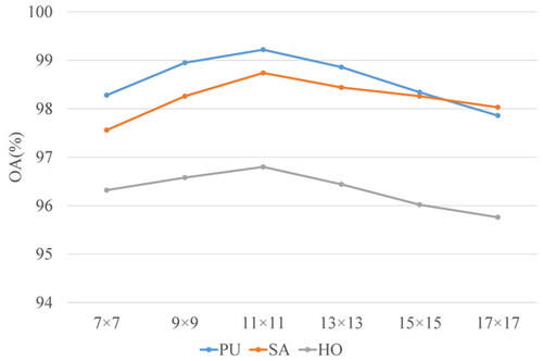
3.3.1. Analysis of the impact of the patch size

In HSI classification, the patch size of the input image is critical to the classification performance of the model. To determine the optimal patch size for the model, we conducted experiments using images with various patch sizes on three real datasets. The patch size ranged from $7\times 7$ to $17\times 17,$ with an interval of 2 pixels. Figure 8 presents the corresponding overall accuracy (OA) values and patch sizes. The results indicate that as the patch size increases, the OA value improves until reaching the peak performance at $11\times 11.$ However, as the patch size continues to increase beyond this point, the OA value significantly decreases. Hence, we set the default parameter as $11\times 11.$ This choice ensures that the model has a sufficient receptive field to extract features while avoiding excessive interference from irrelevant information.

Figure 8. The impact of the patch size on GPHANet is evaluated on three datasets.

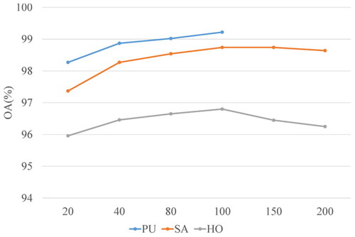
3.3.2. Analysis of the impact of the number of dimensions

We analysed the influence of the number of principal components, denoted as $b,$ on the classification accuracy of the model using the reduced HSI dataset. After applying PCA, the original dataset retains only $b$ bands (principal components). Figure 9 illustrates the relationship between parameter $b$ and the corresponding overall accuracy (OA) values across three datasets. In the case of the Pavia University (PU) dataset, as parameter $b$ increases, the OA value also increases. However, for the Salinas (SA) dataset, which has a higher number of classes and exhibits greater class mixing, retaining a larger number of principal components introduces redundant or even noisy information into the HSI bands, resulting in a slight decrease in classification accuracy. A similar trend is observed in the more complex Houston (HO) dataset. Consequently, we set the default parameter as $b=100$ for all three datasets.

Figure 9. The impact of the principal components $b$ on GPHANet is evaluated on three datasets.

3.4. Classification results

To evaluate the effectiveness of GPHANet, we compared the GPHANet model with SVM (Melgani and Bruzzone 2004), contextual deep CNN (CDCNN) (Lee and Kwon 2017), spectral-spatial residual network (SSRN) (Zhong et al. 2018), DBDA (Li et al. 2020), deformable convolutional residual network (DCRN) (Zhang et al. 2021) and spectral-spatial feature tokenization transformer (SSFTT) (Sun et al. 2022) models. SVM is based on traditional machine learning methods. CDCNN is a deep 2D CNN model that mainly includes 11 convolutional layers and one fully connected layer. SSRM is a serial depth 3DCNN model, and residual connections are introduced to alleviate the degradation problem of the depth model. DBDA is a two-branch 3DCNN model that independently extracts spectral and spatial features. DCRN uses deformable convolution to break the limitations of the fixed receptive field of the standard convolutional kernel. Finally, SSFTT is a hybrid architecture composed of CNN and ViT to extract deep semantic features from HSI. The parameters of these models are consistent with the original paper as much as possible.

Focusing on the PU dataset, we trained the model using 1% of the samples and validated and tested it using the remaining data. The quantitative classification results obtained by different methods are presented in Table 1, and Figure 10 displays the corresponding classification map. The experimental findings indicate that the DL method outperforms SVM in HSI classification. While SVM heavily relies on handcrafted features to represent image attributes like shape and texture, it faces limitations when dealing with complex samples due to the lack of deep semantic feature extraction. Furthermore, CDCNN exhibits the poorest classification performance among the DL methods. This can be attributed to the subtle differences between certain classes in HSI, where the use of 2D convolution alone fails to adequately extract local spatial features for accurate predictions. The degradation of the model resulting from deep networks also affects the classification performance of CDCNN. This issue is effectively addressed by SSRN, which, like CDCNN, is a deep network but employs 3D convolution to extract more discriminative spatial-spectral features. The inclusion of residual connections further mitigates the degradation problem. In the case of DBDA and DCRN, which belong to the multi-branch 3DCNN model, the deformable convolution in DCRN enables adaptive feature detection across different spatial locations and an expanded receptive field, leading to improved classification results. SSFTT, based on ViT with a global receptive field and self-attention mechanism, does not achieve top performance in HSI data. This is due to the self-attention mechanism considering relationships between all elements in the input data. When the number of training samples is limited, this global computation can result in overfitting, as the model becomes overly reliant on individual input elements without generalizing from a broader context. In contrast, GPHANet incorporates the HAM, which utilizes content-based attention to capture specific input element relationships within a context window, enabling selective attention to relevant information. Overall, GPHANet achieves the highest classification accuracy in terms of OA, AA, and Kappa. It effectively preserves detailed HSI information across various scales, from global to local, and strikes a relative balance between depth and width, effectively mitigating the overfitting problem.

Figure 10. Visual comparison on the PU dataset: (a) Ground-truth, (b) SVM, (c) CDCNN, (d) SSRN, (e) DBDA, (f) DCRN, (g) SSFTT, (h) GPHANet.

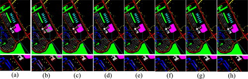
Table 1. Classification results of seven methods on the PU dataset.

Classes	SVM	CDCNN	SSRN	DBDA	DCRN	SSFTT	GPHANet
	89.85	89.95	99.14	96.20	97.63	98.89	98.50
	92.80	97.69	99.15	99.78	99.76	99.85	99.74
	69.90	91.88	82.46	98.07	97.81	95.66	98.52
	93.96	99.58	100	99.45	98.21	98.50	98.06
	98.44	99.77	98.59	99.32	99.84	99.08	99.47
	85.00	92.48	99.89	99.51	99.47	99.73	99.90
	73.15	74.27	90.08	99.73	99.12	93.82	100
	80.69	88.95	92.10	99.05	95.33	96.22	98.50
	99.25	95.76	100	99.12	99.77	97.32	97.04
OA	88.92	94.26	97.48	98.62	98.80	98.79	99.22
AA	87.08	92.26	95.72	98.47	98.55	97.68	98.86
Kappa	85.23	92.38	96.62	98.17	98.39	98.41	98.97

On the SA dataset, we trained the model using only 1% of the samples. The quantitative classification results obtained by different methods are shown in Table 2, and the corresponding classification map is visualized in Figure 11. GPHANet achieves the highest OA, AA, and Kappa values, even for classes with high spectral similarity in the SA dataset. In addition, GPHANet provides a classification map that is most consistent with ground truth, with less noise and clearer object edges. For the HO datasets, we trained the model using only 0.5% of the samples. The quantitative classification results obtained by different methods are reported in Table 3, and the corresponding classification map is visualized in Figure 12. Compared to the PU and SA datasets, the HO datasets feature more complex mixtures of classes and significant variations in spatial representations between classes, posing greater challenges for classification. Nevertheless, GPHANet consistently outperforms other classification methods, demonstrating its robustness in handling such challenging scenarios.

Figure 11. Visual comparison on the SA dataset: (a) Ground-truth, (b) SVM, (c) CDCNN, (d) SSRN, (e) DBDA, (f) DCRNet, (g) SSFTT, (h) GPHANet.

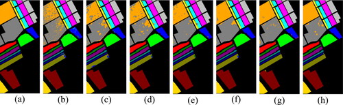
Figure 12. Visual comparison on the HO dataset: (a) Ground-truth, (b) SVM, (c) CDCNN, (d) SSRN, (e) DBDA, (f) DCRN, (g) SSFTT, (h) GPHANet.

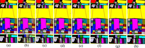
Table 2. Classification results of seven methods on the SA dataset.

Classes	SVM	CDCNN	SSRN	DBDA	DCRN	SSFTT	GPHANet
	99.95	99.70	99.59	100	100	99.64	100
	97.94	99.67	99.95	100	100	99.65	100
	88.60	86.78	95.45	99.38	96.47	100	99.64
	95.73	95.68	97.21	89.95	99.55	96.09	100
	95.64	98.25	99.73	99.96	98.83	97.75	98.46
	99.85	98.03	99.97	100.00	100	99.89	100
	99.32	98.92	99.49	99.80	99.43	100	100
	77.30	89.43	91.24	95.06	98.50	99.28	99.01
	99.31	99.61	99.98	99.46	99.98	100	99.95
	88.39	92.89	96.36	96.52	99.55	97.44	99.41
	81.49	84.49	90.33	93.11	98.02	100	100
	97.69	99.26	99.37	100	99.47	93.79	99.47
	94.44	99.67	98.24	99.89	99.88	99.77	99.44
	93.71	99.14	98.49	96.96	98.59	99.71	100
	75.15	82.22	83.28	94.98	92.13	94.49	93.68
	97.71	99.76	99.65	99.83	100	100	99.77
OA	89.51	93.59	96.24	97.49	98.25	98.42	98.74
AA	92.63	95.21	96.77	97.81	98.81	98.59	99.30
Kappa	88.30	92.87	94.48	97.20	98.06	98.24	98.59

Table 3. Classification results of seven methods on the HO dataset.

Classes	SVM	CDCNN	SSRN	DBDA	DCRN	SSFTT	GPHANet
	93.68	97.13	99.02	98.48	99.32	98.66	96.79
	63.81	82.68	96.06	75.01	84.57	90.51	80.52
	79.18	88.67	94.41	90.56	94.55	93.81	94.99
	92.06	98.65	98.95	99.39	99.39	99.04	99.44
	57.31	84.59	93.81	80.68	83.34	89.10	95.52
	82.58	95.14	95.56	98.84	97.52	99.01	98.59
	63.64	83.42	89.87	93.60	87.09	92.63	94.41
	26.07	48.74	70.70	81.48	83.41	85.32	88.45
	95.16	96.53	97.68	99.20	99.38	99.48	98.27
	67.81	90.02	77.76	92.02	99.08	92.41	97.07
	56.72	80.25	87.27	95.63	94.89	96.25	96.96
	56.58	62.72	67.58	94.00	89.06	81.05	87.18
	60.62	82.97	86.15	84.16	91.88	88.11	88.17
	89.47	86.20	90.22	98.04	96.86	93.20	97.43
	88.10	96.51	71.20	100.00	97.66	79.75	95.10
	78.42	89.67	93.30	89.31	99.76	94.81	99.50
	70.99	72.99	87.56	94.34	79.08	90.88	87.21
	53.35	78.29	89.99	98.56	92.37	86.31	94.88
	77.81	91.13	88.46	87.92	89.77	91.47	99.27
	68.99	88.37	88.15	95.58	97.07	86.15	93.82
	20.00	37.54	64.50	74.91	83.56	81.98	87.83
	49.59	89.57	94.95	94.84	94.39	93.10	90.16
OA	82.20	91.67	93.86	95.57	96.06	95.80	96.80
AA	70.99	82.81	87.42	91.66	92.45	91.05	93.70
Kappa	76.07	89.82	92.33	94.40	95.02	94.69	95.95

In addition, to evaluate the efficiency of the model, we further compared the testing time among different methods as shown in Table 4. Since SVM requires very little time when testing on fewer samples but performs poorly in terms of classification accuracy, it is not included in the table. It can be observed that GPHANet achieves satisfactory results in terms of testing time on all three datasets. Although DCRN achieves good classification results, the use of deformable convolutions introduces an additional computational burden, resulting in significantly higher testing time compared to other methods. SSFTT utilizes a combination of 2D and 3D convolutions for spatial and spectral feature extraction, and its time cost is slightly lower than our method. Overall, GPHANet strikes a balance between performance and efficiency, achieving higher classification accuracy with less time consumption.

Table 4. The testing time (s) between different methods on three datasets.

Dataset	SVM	CDCNN	SSRN	DBDA	DCRN	SSFTT	GPHANet
PU	–	4.36	14.42	22.21	29.56	10.11	14.96
SA	–	6.74	23.39	36.68	43.04	18.72	26.15
HO	–	74.23	195.77	354.63	392.18	183.05	231.54

4. Discussion

4.1. Effectiveness of different modules in GPHANet

In this section, to evaluate the effectiveness of each module in GPHANet, we conducted a series of ablation experiments on three data sets.

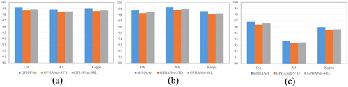
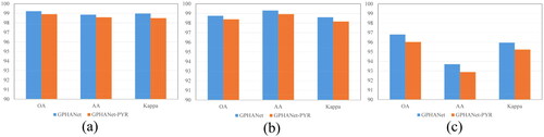
The first experiment was performed on the GSSCM module. Specifically, we replace the global spatial spectral convolution in GSSCM with the standard convolution. In addition, we compare the composition of global convolution in GSSCM, including series and parallel structures. The experimental results are shown in Figure 13. GPHANet-STD indicates that the GSSCM of GPHANet uses only standard convolutions. On the other hand, GPHANet-SRL represents the combination of multiple global convolutions in the GSSCM, arranged in a serial structure. It can be seen that the classification performance using global convolution is better than that using standard convolution. The OA, AA, and Kappa values on the PU dataset are +0.55%, +0.47%, and +0.41%, respectively. The global convolution can capture information from the entire input space, thereby extracting higher semantic-level features. The situation is similar in SA and HO datasets. In addition, compared to serial structures, parallel structures encourage a wider representation of features from input to output, which alleviates the degradation of deep networks while ensuring the classification performance of the model. Comparative experiments of the convolution mechanism and combination method prove the effectiveness of the proposed GSSCM.

Figure 13. The effectiveness of GSSCM on three datasets, (a) PU, (b) SA, (c) HO.

To evaluate the effectiveness of DPCM, we conducted a second experiment where we removed the dynamic routing module from DPCM and analysed the impact on the overall accuracy (OA) values. In this scenario, only pyramid convolutions were employed to extract multiscale features. The experimental results are depicted in Figure 14. GPHANet-PYR indicates that the DPCM of GPHANet uses only pyramid convolutions. The removal of the dynamic routing module led to a decline in the classification performance across the three datasets. Particularly on the HO dataset, there was a significant reduction in classification accuracy. This can be attributed to the fact that the HO dataset contains a higher degree of the class mixture and significant variations in spatial representations among classes. Compared to standard pyramid convolution operations, our proposed dynamic pyramid convolution overcomes the limitations of static convolutions by enabling adaptive parameter adjustment of convolutional kernels at different scales based on input. This facilitates more precise and detailed multiscale feature extraction.

Figure 14. The effectiveness of DPCM on three datasets, (a) PU, (b) SA, (c) HO.

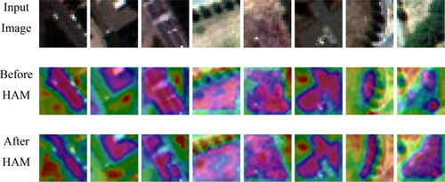
Finally, GPHANet applies HAM to fuse the global and local features extracted from the two branches to generate global-local spatial-spectral features. Therefore, we evaluate the effectiveness of HAM by comparing different feature fusion methods. The fusion methods involved in the comparison include the HAM proposed in this article and the Concat and Sum widely used in existing work. Figure 15 reports the experimental results on three data sets. It can be observed that HAM consistently provides the highest OA value. Compared to Concat, the OA values on the three data are +0.43%, +0.51%, and +0.54%, respectively. The results compared to Sum are similar. HAM employs a three-branch structure to capture cross-dimensional interaction information and calculate attention weights, which can adaptively highlight the most important hyperspectral features for classification while reducing the interference of noise information. Each weight generated by HAM includes spectral information, horizontal spatial information, and vertical spatial information, which can effectively improve the expression ability of the model. We also utilize the Score-CAM (Ibrahim and Shafiq 2022) method to visualize the feature maps generated by GPHANet, as shown in Figure 16. By comparing the feature maps before and after HAM, it can be demonstrated that HAM can effectively help the model in locating objects of interest.

Figure 15. The effectiveness of HAM on three datasets, (a) PU, (b) SA, (c) HO.

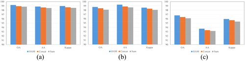
Figure 16. Visualization of the feature maps generated before and after HAM.

4.2. Sensitivity to the number of training samples

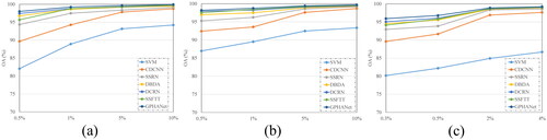
This experiment analysed the classification performance of different models using different proportions of training samples. Specifically, on the PU and SA datasets, 0.5%, 1%, 5%, and 10% of training samples are selected, and on the HO dataset, 0.3%, 0.5%, 2%, and 4% of training samples are selected. The experimental results are shown in Figure 17. From the results, it can be found that with the increase of training samples, the performance of the model based on DL has been significantly improved in all three data sets. This is because traditional machine learning models are based on handcraft features, while DL models can automatically learn high-level semantic features from images. In addition, the performance of the proposed GPHANet is better than that of the comparison model, indicating that using both global context information and local multiscale information can effectively improve the classification performance of the algorithm. In addition, GPHANet can automatically adjust the parameters of convolutional kernels with different scales based on different inputs, which can achieve better performance when training samples are constantly changing, making the model more robust and adaptive.

Figure 17. OA results of seven methods under different proportions of training samples: (a) PU, (b) SA, (C) HO.

5. Conclusions

In this work, we proposed a new DL-based network called GPHANet for HSI classification. To overcome the limitations of limited receptive fields and boundary effects, we adopt the design of multiple asymmetric and circular convolutions with a global receptive field in GSSCM. As a result, every position of the convolutional layer in GSSCM can receive all information from the entire input space. In addition, the DPCM is proposed to achieve more accurate and detailed multiscale feature extraction. Furthermore, the HAM is implemented to highlight the most useful spatial and spectral information for classification, while suppressing irrelevant information. Based on these approaches, GPHANet extracts features at both global and local levels, leveraging the rich information in HSI and obtaining more robust and discriminative feature representations. The proposed model achieved impressive overall accuracies of 99.22%, 98.74%, and 96.80% on the Pavia University, Salinas, and Hong Hu datasets, respectively, using limited training samples, which are much better compared to the state-of-the-art methods. To balance performance and efficiency, our method utilizes the PCA dimensionality reduction, which may lead to the loss of some detailed information in the reduced data. Therefore, improving the computational efficiency of the global convolution across full spectral bands is one of our future works. In addition, the proposed GPHANet exhibits good scalability in extracting global and local features from multimodal data. Therefore, we will apply the proposed model for the joint fusion and classification of hyperspectral and LiDAR data.

Disclosure statement

The authors declared that they have no conflicts of interest in this work.

References

- Alsallakh B, Kokhlikyan N, Miglani V, Yuan J, Reblitz-Richardson O. 2020. Mind the Pad–CNNs can develop blind spots. arXiv preprint arXiv:201002178. doi: 10.48550/arXiv.2010.02178.
- Bing L, Xuchu Y, Pengqiang Z, Xiong T. 2019. Deep 3D convolutional network combined with spatial-spectral features for hyperspectral image classification. Acta Geod Cartogr Sinica. 48(1):53.
- Chen Y, Dai X, Liu M, Chen D, Yuan L, Liu Z. 2020. Dynamic convolution: attention over convolution kernels. In: 2020 IEEE/CVF Conference on Computer Vision and Pattern Recognition (CVPR); Jun 2020. p. 11027–11036. doi: 10.1109/CVPR42600.2020.01104.
- Ding Y, Zhao X, Zhang Z, Cai W, Yang N. 2021. Multiscale graph sample and aggregate network with context-aware learning for hyperspectral image classification. IEEE J Sel Top Appl Earth Observ Remote Sens. 14:4561–4572. doi: 10.1109/JSTARS.2021.3074469.
- Dong Y, Liu Q, Du B, Zhang L. 2022. Weighted feature fusion of convolutional neural network and graph attention network for hyperspectral image classification. IEEE Trans Image Process. 31:1559–1572. doi: 10.1109/TIP.2022.3144017.
- Du Y, Jiang J, Liu Z, Pan Y. 2022. Combining a crop growth model with CNN for underground natural gas leakage detection using hyperspectral imagery. IEEE J Sel Top Appl Earth Observ Remote Sens. 15:1846–1856. doi: 10.1109/JSTARS.2022.3150089.
- Duta IC, Liu L, Zhu F, Shao L. 2020. Pyramidal convolution: rethinking convolutional neural networks for visual recognition. arXiv preprint arXiv:200611538. doi: 10.48550/arXiv.2006.11538.
- Feng J, Zhao N, Shang R, Zhang X, Jiao L. 2022. Self-supervised divide-and-conquer generative adversarial network for classification of hyperspectral images. IEEE Trans Geosci Remote Sens. 60:1–17. doi: 10.1109/TGRS.2022.3202908.
- Fu J, Liu J, Tian H, Li Y, Bao Y, Fang Z, Lu H. 2019. Dual attention network for scene segmentation. In: 2019 IEEE/CVF Conference on Computer Vision and Pattern Recognition (CVPR); June 2019. p. 3141–3149. doi: 10.1109/CVPR.2019.00326.
- Ge H, Wang L, Liu M, Zhu Y, Zhao X, Pan H, Liu Y. 2023. Two-branch convolutional neural network with polarized full attention for hyperspectral image classification. Remote Sens. 15(3):848. doi: 10.3390/rs15030848.
- Ghaderizadeh S, Abbasi-Moghadam D, Sharifi A, Tariq A, Qin S. 2022. Multiscale dual-branch residual spectral–spatial network with attention for hyperspectral image classification. IEEE J Sel Top Appl Earth Observ Remote Sens. 15:5455–5467. doi: 10.1109/JSTARS.2022.3188732.
- Gu Y, Liu T, Jia X, Benediktsson JA, Chanussot J. 2016. Nonlinear multiple kernel learning with multiple-structure-element extended morphological profiles for hyperspectral image classification. IEEE Trans Geosci Remote Sens. 54(6):3235–3247. doi: 10.1109/TGRS.2015.2514161.
- Haut JM, Paoletti ME, Plaza J, Plaza A, Li J. 2019. Visual attention-driven hyperspectral image classification. IEEE Trans Geosci Remote Sens. 57(10):8065–8080. doi: 10.1109/TGRS.2019.2918080.
- Hong D, Han Z, Yao J, Gao L, Zhang B, Plaza A, Chanussot J. 2022. SpectralFormer: rethinking hyperspectral image classification with transformers. IEEE Trans Geosci Remote Sens. 60:1–16. doi: 10.1109/TGRS.2021.3130716.
- Hou Q, Zhang L, Cheng MM, Feng J. 2020. Strip pooling: rethinking spatial pooling for scene parsing. In: 2020 IEEE/CVF Conference on Computer Vision and Pattern Recognition (CVPR); June 2020. p. 4002–4011. doi: 10.1109/CVPR42600.2020.00406.
- Hou Q, Zhou D, Feng J. 2021. Coordinate attention for efficient mobile network design. In: 2021 IEEE/CVF Conference on Computer Vision and Pattern Recognition (CVPR); June 2021. p. 13708–13717. doi: 10.1109/CVPR46437.2021.01350.
- Hu W, Huang Y, Wei L, Zhang F, Li H. 2015. Deep convolutional neural networks for hyperspectral image classification. J Sens. 2015:1–12. doi: 10.1155/2015/258619.
- Hu W, Li H, Deng Y, Sun X, Du Q, Plaza A. 2021. Lightweight tensor attention-driven ConvLSTM neural network for hyperspectral image classification. IEEE J Sel Top Signal Process. 15(3):734–745. doi: 10.1109/JSTSP.2021.3063805.
- Ibrahim R, Shafiq MO. 2022. Augmented score-CAM: high resolution visual interpretations for deep neural networks. Knowledge-Based Syst. 252:109287. doi: 10.1016/j.knosys.2022.109287.
- Jay S, Guillaume M. 2014. A novel maximum likelihood based method for mapping depth and water quality from hyperspectral remote-sensing data. Remote Sens Environ. 147:121–132. doi: 10.1016/j.rse.2014.01.026.
- Kang X, Zhuo B, Duan P. 2019. Dual-path network-based hyperspectral image classification. IEEE Geosci Remote Sens Lett. 16(3):447–451. doi: 10.1109/LGRS.2018.2873476.
- Kayhan OS, Gemert JCv. 2020. On translation invariance in CNNs: convolutional layers can exploit absolute spatial location. In: 2020 IEEE/CVF Conference on Computer Vision and Pattern Recognition (CVPR); 13-19 June 2020.
- Khan A, Vibhute AD, Mali S, Patil CH. 2022. A systematic review on hyperspectral imaging technology with a machine and deep learning methodology for agricultural applications. Ecol Inf. 69:101678. doi: 10.1016/j.ecoinf.2022.101678.
- Kumar B, Dikshit O. 2017. Hyperspectral image classification based on morphological profiles and decision fusion. Int J Remote Sens. 38(20):5830–5854. doi: 10.1080/01431161.2017.1348636.
- Lee H, Kwon H. 2017. Going deeper with contextual CNN for hyperspectral image classification. IEEE Trans Image Process. 26(10):4843–4855. doi: 10.1109/TIP.2017.2725580.
- Li Y, Kuang Z, Chen Y, Zhang W. 2019. Data-driven neuron allocation for scale aggregation networks. In: 2019 IEEE/CVF Conference on Computer Vision and Pattern Recognition (CVPR). Jun 2019. p. 11518–11526. doi: 10.1109/CVPR.2019.01179.
- Li R, Zheng S, Duan C, Yang Y, Wang X. 2020. Classification of hyperspectral image based on double-branch dual-attention mechanism network. Remote Sensing. 12(3):582. doi: 10.3390/rs12030582.
- Li Z, Cui X, Wang L, Zhang H, Zhu X, Zhang Y. 2021. Spectral and spatial global context attention for hyperspectral image classification. Remote Sens. 13(4):771. doi: 10.3390/rs13040771.
- Liu Y, Li X, Hua Z, Xia C, Zhao L. 2022. A band selection method with masked convolutional autoencoder for hyperspectral image. IEEE Geosci Remote Sens Lett. 19:1–5. doi: 10.1109/LGRS.2022.3178824.
- Liu H, Li W, Xia XG, Zhang M, Gao CZ, Tao R. 2022. Central attention network for hyperspectral imagery classification. IEEE Trans Neural Netw Learning Syst. [accessed 2022 March 10]:[15 p.]. doi: 10.1109/TNNLS.2022.3155114.
- Melgani F, Bruzzone L. 2004. Classification of hyperspectral remote sensing images with support vector machines. IEEE Trans Geosci Remote Sens. 42(8):1778–1790. doi: 10.1109/TGRS.2004.831865.
- Mou L, Zhu XX. 2020. Learning to pay attention on spectral domain: a spectral attention module-based convolutional network for hyperspectral image classification. IEEE Trans Geosci Remote Sens. 58(1):110–122. doi: 10.1109/TGRS.2019.2933609.
- Nie J, Xu Q, Pan J, Guo M. 2022. Hyperspectral image classification based on multiscale spectral–spatial deformable network. IEEE Geosci Remote Sens Lett. 19:1–5. doi: 10.1109/LGRS.2020.3024006.
- Niu Z, Zhong G, Yu H. 2021. A review on the attention mechanism of deep learning. Neurocomputing. 452:48–62. doi: 10.1016/j.neucom.2021.03.091.
- Shah C, Du Q, Xu Y. 2022. Enhanced TabNet: attentive interpretable tabular learning for hyperspectral image classification. Remote Sens. 14(3):716. doi: 10.3390/rs14030716.
- Shi H, Cao G, Ge Z, Zhang Y, Fu P. 2021. Double-branch network with pyramidal convolution and iterative attention for hyperspectral image classification. Remote Sens. 13(7):1403. doi: 10.3390/rs13071403.
- Sun L, Zhao G, Zheng Y, Wu Z. 2022. Spectral–spatial feature tokenization transformer for hyperspectral image classification. IEEE Trans Geosci Remote Sens. 60:1–14. doi: 10.1109/TGRS.2022.3144158.
- Szegedy C, Ioffe S, Vanhoucke V, Alemi A. 2017. Inception-v4, Inception-ResNet and the impact of residual connections on learning. AAAI. 31(1):4278–4284. doi: 10.1609/aaai.v31i1.11231.
- Wang J, Huang R, Guo S, Li L, Zhu M, Yang S, Jiao L. 2021. NAS-guided lightweight multiscale attention fusion network for hyperspectral image classification. IEEE Trans Geosci Remote Sens. 59(10):8754–8767. doi: 10.1109/TGRS.2021.3049377.
- Wang Q, Wu B, Zhu P, Li P, Zuo W, Hu Q. 2020. ECA-Net: efficient channel attention for deep convolutional neural networks. In: 2020 IEEE/CVF Conference on Computer Vision and Pattern Recognition (CVPR); June 2020. p. 11531–11539. doi: 10.1109/CVPR42600.2020.01155.
- Wieme J, Mollazade K, Malounas I, Zude-Sasse M, Zhao M, Gowen A, Argyropoulos D, Fountas S, Van Beek J. 2022. Application of hyperspectral imaging systems and artificial intelligence for quality assessment of fruit, vegetables and mushrooms: a review. Biosyst Eng. 222:156–176. doi: 10.1016/j.biosystemseng.2022.07.013.
- Xu Y, Zhang L, Du B, Zhang F. 2018. Spectral–spatial unified networks for hyperspectral image classification. IEEE Trans Geosci Remote Sens. 56(10):1–17. doi: 10.1109/TGRS.2018.2827407.
- Yang Y, Qu J, Xiao S, Dong W, Li Y, Du Q. 2022. A deep multiscale pyramid network enhanced with spatial–spectral residual attention for hyperspectral image change detection. IEEE Trans Geosci Remote Sens. 60:1–13. doi: 10.1109/TGRS.2022.3161386.
- Yu C, Han R, Song M, Liu C, Chang C-I. 2020. A simplified 2D-3D CNN architecture for hyperspectral image classification based on spatial–spectral fusion. IEEE J Sel Top Appl Earth Observ Remote Sens. 13:2485–2501. doi: 10.1109/JSTARS.2020.2983224.
- Zhang H, Hu W, Wang X. 2022. ParC-Net: position aware circular convolution with merits from ConvNets and transformer. Computer Vision-ECCV 2022; Oct 2022. p. 613–630. doi: 10.1007/978-3-031-19809-0_35.
- Zhang T, Shi C, Liao D, Wang L. 2021. A spectral spatial attention fusion with deformable convolutional residual network for hyperspectral image classification. Remote Sens. 13(18):3590. doi: 10.3390/rs13183590.
- Zhao C, Zhu W, Feng S. 2022. Hyperspectral image classification based on kernel-guided deformable convolution and double-window joint bilateral filter. IEEE Geosci Remote Sens Lett. 19:1–5. doi: 10.1109/LGRS.2021.3084203.
- Zhong Z, Li J, Luo Z, Chapman M. 2018. Spectral–spatial residual network for hyperspectral image classification: a 3-D deep learning framework. IEEE Trans Geosci Remote Sens. 56(2):847–858. doi: 10.1109/TGRS.2017.2755542.
- Zhou W, Kamata S, Luo Z, Wang H. 2022. Multiscanning strategy-based recurrent neural network for hyperspectral image classification. IEEE Trans Geosci Remote Sens. 60:1–18. doi: 10.1109/TGRS.2021.3138742.