Automated analysis of snowmelt from Sentinel-2 imagery to determine variable rate irrigation zones in the American Mountain West

Abstract

Variable rate irrigation (VRI) is used to save water whilst maintaining crop yields in semiarid regions. A key problem is to be able to inexpensively determine spatial patterns in soil moisture so that VRI zones can be defined. In Southern Idaho, USA, the annual precipitation is low and most fall as winter snow. This research investigates whether snow melt patterns measured using freely available time-series Sentinel 2 imagery from Google Earth Engine can define useful VRI zones for two arable fields (Grace and Rexburg). The normalized difference snow index (NDSI) was computed for each 10 m pixel with snow for all winter images of the fields for 2018–2022. NDSI values were ranked within each image and average ranks were calculated for each month and over several years. The patterns of March NDSI were most similar to patterns in yield and soil moisture observed in previous years. Zones were determined using K-means classification of the mean ranks of March NDSI. Kruskal Wallis H tests showed consistent and significant differences between zones for key soil, plant, and topographic variables. For the Grace site, differences between zones were more consistent in their order of magnitude than VRI zones which were calculated using a labor-intensive method. For the Rexburg site, zones were shown to be better when based on snowmelt data from March 2018 to 2022 rather than just March 2019. It is important to base zones on several years of data because in some years there was no snow observed in the Grace field in March. In locations where the majority of soil moisture comes from snowmelt, basing VRI zones on several years of snowmelt patterns in March is a useful and inexpensive tool for deriving meaningful VRI zones. The code used to automatically extract suitable sentinel images and calculate the NDSI is included so that practitioners can use this approach in other locations.

Keywords:

• Normalized difference snow index
• Sentinel 2 imagery
• variable rate irrigation
• management zones
• google earth engine

1. Introduction

The agricultural sector is the biggest user of fresh water in the USA (>80%) (Wiebe and Gollehon 2006). Variable rate irrigation (VRI) of crops is a promising approach for saving water whilst maintaining crop yields in the semi-arid American Mountain West. Studies have shown that improvements in water use efficiency of at least 17–39% can be achieved (Cohen et al. 2021). Using VRI is currently particularly important in the Mountain West region as it is experiencing a ‘mega drought’ (Williams et al. 2022) with >30% of the western USA currently categorized as having extreme or exceptional drought (Drought Monitor 2023). However, to achieve the maximum improvements in water use efficiency possible with a VRI system, accurate irrigation management zones must be identified within fields (Khosla et al. 2008; O’Shaughnessy et al. 2019). Characterizing spatial variation in soil moisture and other key variables (e.g. crop yield, topography, and soil texture) to determine if the spatial patterns are relatively stable temporally is the first step towards determining suitable management zones.

Soil moisture is water available in the pores of the soil, and it is not dependent on rivers, lakes, or groundwater (Larson et al. 2022). Characterizing VRI zones is done using ancillary data that relate to the variations in soil moisture and other key variables like yield. Once zones are defined, soil moisture sensors are installed in each zone. Research has found there is significant spatial and temporal variability in soil moisture within VRI zones, and further research is needed to identify optimal placement of soil moisture sensors within zones (Woolley et al. 2021). Accurately mapping soil moisture levels involves expensive and time-consuming field and lab work. The goal with VRI is to maintain yield and use less freshwater while increasing profitability. However, expensive field and lab work can reduce profitability so cheaper methods of inferring patterns of soil moisture are needed. Key to understanding patterns of soil moisture is being able to characterize how patterns of soil moisture are likely to vary with topography and soil texture. Spatial patterns of soil moisture are usually influenced by topography (Oroza et al. 2018). Ortiz et al. (2022) therefore investigated if topographic indices could be used for defining VRI zones. Also, where snow is a significant source of soil moisture, snow cover and its melt are important to understanding patterns of soil moisture (Choubin, Roshan, et al. 2019; Nyamgerel et al. 2022).

In Southern Idaho, one of the main agricultural areas in the American Mountain West, annual precipitation levels are typically <500 mm with most falling as winter snow or spring rain. Svedin et al. (2021) noted that in such locations winter snowfall and spring thaw act as the principal wetting event and that the variation of water content at spring green-up seems to be a function of snow accumulation and melting patterns over the winter and early spring. A logical extension of this is that snow accumulation and melting patterns are likely to be related to micro-topographic features such as aspect. Aspect influences the amount of insolation received at each location and will also influence the water needs of the crop during the season and the final crop yield.

Using a time-series of freely available remotely sensed data is probably the easiest way to analyze patterns of snowmelt. However, the first step in such analysis would be identifying which pixels have snow and which do not. The term Normalized Difference Snow Index (NDSI) was first used by Hall et al. (1995) but similar methods have been used to map and separate snow from clouds since the mid-1970s (Hall and Riggs 2007). Most studies have used the NDSI calculated from different satellite remote sensing products to monitor snow cover in mountainous areas to infer variability in the water supply and increased melting rates associated with global warming (Lin et al. 2012; Sharma et al. 2012; Choubin, Solaimani, et al. 2019; Nagajothi et al. 2019; Zhang et al. 2021). It has also been used to monitor how pollutants landing on the snow surface alter the albedo effect of the snow (Dozier et al. 2009), to glean snowline elevations in mountainous areas (Choubin, Alamdarloo, et al. 2019), to estimate snow cover in forested areas (Shimamura et al. 2006), and as an input to classify watersheds with similar hydrologic characteristics (Choubin, 2017). Smith et al. (2021) reviewed approaches that have been used for developing VRI zones and advocated approaches based on various wavebands from satellite remote sensing products. To our knowledge analysis of snowmelt patterns using satellite remote sensing or NDSI to determine zones has not previously been investigated for the purposes of precision agriculture or precision irrigation.

This research modifies existing code to automatically extract time-series Sentinel 2 imagery from Google Earth Engine and calculate and analyze patterns in NDSI for different months and seasons/years. This paper has two objectives. The first objective was to determine if modified Google Earth Engine code and data can be reliably used to measure time-series NDSI data. The second objective was to determine what months and seasons of NDSI data could be used to produce meaningful VRI zones that show significant differences in spring soil moisture and other key variables like yield, aspect, etc. The study focuses on two field sites in Southern Idaho. Dense soil sampling followed by laboratory determination of soil moisture content and other related variables has been undertaken at both sites to allow accurate geostatistical mapping of soil moisture patterns in the fields. Yield data were also collected along with a digital elevation model (DEM) from the global positioning system (GPS) attached to the yield monitor. All these variables are compared between zones developed using NDSI and zones used by Woolley et al. (2021) in one of the fields. The zones of Woolley et al. (2021) were developed using soil moisture and other data and a more labor and computationally-intensive approach. For the other field, the NDSI zones developed using one season of data are compared to those produced using 5 years of data.

2. Methods

2.1. Field sites and data collection

Data were collected at two arable field sites in Southern Idaho, USA (Figure 1) that had central pivot irrigation systems installed. The first site, which forms the main focus of this study, was located near Grace, Caribou County, Idaho (elevation 1687 m above sea level; 42.60904 latitude and −111.788 longitude) (Woolley et al. 2021). It is a 22-ha semi-circular agricultural field covering the northern half of a central pivot. The southern part of the central pivot is a golf course. A wheat-wheat-potato crop rotation is employed in the field. The soil series is Rexburg-Ririe complex with 1–4% slopes and has a consistent silty clay loam texture throughout the field. The climate of Southern Idaho, a semi-arid region, is typified by relatively hot days and cool nights during the summer growing season. Average annual precipitation is 390 mm with the majority occurring as winter snow, which often blows and accumulates variably based on topography and surface soil tillage/plant residue (Woolley et al. 2021). The variation of elevation within the field (Figure 2(b)) shows only about a 7 m difference in the highest and lowest elevation locations, but a key feature of the elevation patterns is a west-facing slope that bi-sects the middle of the field.

The Grace field was studied in the 2016–2021 growing seasons. During that time the crops were: 2016 – wheat, 2017 – wheat, 2018 – potato, 2019 – wheat, 2020 – wheat and 2021 – potato. Wheat yield data were collected using a mass-based yield sensor equipped with a GPS located on the combine. Yield data were pre-processed before mapping to remove artefacts related to double passes of the combine over certain areas etc. A DEM was developed from the elevations associated with the GPS locations from yield monitoring. Saga GIS (Conrad et al. 2015) was used to compute derived topographic attributes such as aspect, slope and topographic wetness index (TWI) from the DEM. During each of the 6 growing seasons (2016–2021), 85–102 soil samples were collected throughout the field (Figure 2(a)). For the earlier seasons, samples were collected in Spring and Fall, but samples were collected up to four times in later growing seasons. Soil samples were collected at four depths (0–0.3 m, 0.3–0.6 m, 0.6–0.9 m, and 0.9–1.2 m) using a modified gas-powered post driver (Art’s Manufacturing and Supply (AMS), Inc. American Falls, ID, USA). Gravimetric water content of the soil was determined by drying in a forced air oven at 105 °C until consistent weights were reached. Gravimetric water contents were converted to volumetric water contents (VWC, %) using soil bulk density values determined in 2016 (Svedin et al. 2021). Evapotranspiration (ET) levels (mm) were modelled at different times using the Penman-Monteith equation (Allen et al. 1998).

At the Grace site, irrigation zones (Woolley et al. 2021) were developed in 2019 by analyzing patterns in 2016 and 2017 crop water productivity (CWP, %). Crop water productivity is determined by dividing yield by ET, or the amount of water supplied. Defining the irrigation zones based on CWP was accomplished by using a regression where yield was the response variable and ET was the explanatory variable. Finally, a k-means clustering algorithm with constraints for spatial contiguity was used to map out the five irrigation zones (Woolley et al. 2021). These zones seem to be effective, but they are based on very labor-intensive data collection and analysis. ET calculations were derived from soil moisture measurements from 102 locations at 4 depths taken two-four times throughout the growing season. These irrigation zones are hereafter referred to as the Woolley et al. (2021) zones and are shown as the black lines in Figure 2(a). They were used as a comparison for the zones developed using the automated time-series snow-melt analysis.

2.2. Coding and development of automated image extraction

Sentinel 2 imagery was chosen for this analysis as it is freely available through Google Earth Engine, has a frequent revisit time of 5 days, has a relatively small pixel size (10 m) and captures suitable wavelengths for calculating the normalized difference snow index (NDSI). Landsat thematic mapper data are also freely available and have wavelengths suitable for computing the NDSI (ieee.org/document/399618), however, the moderate spatial resolution with 30 m pixels for most wavebands (Mulla 2021) makes it a little coarse for spatial analysis within individual agricultural fields for precision agriculture. Oliver (2013) noted that the optimal resolution for imagery data for precision agriculture studies is 2–5 m pixels. Also, the longer revisit time for Landsat (16 days) makes it unlikely that multiple occurrences of snow will be observed each month to make a time series of data. The equation for the NDSI is: (1) $$\text{NDSI = }\left(\text{Green }\mathrm{–}\text{ SWIR 1}\right)\text{/}\left(\text{Green + SWIR 1}\right).$$(1)

For Sentinel 2 imagery, Green = Band 3 and SWIR 1 = Band 11. NDSI is based on snow reflecting strongly in the green band, but it is absorbed strongly in the shortwave infrared band. The NDSI algorithm in combination with near-infrared reflectance is used to identify snow cover and discriminate snow from clouds. The algorithm functions with a simple set of decision rules for snow and can be run in an automated fashion without prior knowledge of surface characteristics (Riggs et al. 1994; IEEE, 2023). The NDSI value for each pixel relates to the percent coverage of that pixel by snow. If NDSI >0, there is snow in that pixel, if the NDSI value is 0.5, 50% of the pixel is covered in snow and if NDSI = 1, the pixel is completely covered in snow. The surface reflectance (SR) data were used here rather than the top of atmosphere (TOA) as snow presence is a feature of surface reflectance.

Existing Github code, namely the color palette and the spectral index repository (Github palettes 2023; Github spectral-indices 2023) was modified to select suitable Sentinel images from the desired time frame, for the study sites and calculate the NDSI. This process of selecting Sentinel imagery and calculating the NDSI is summarized in a flow diagram (Figure 3). A more detailed description of the process and code used to (1) extract images with <40% cloud cover and sufficient snow cover (i.e. max. NDSI value > 0.5) for the study sites and (2) calculate the NDSI, is provided with explanations in Appendix A.

NDSI images processed in GEE were downloaded and brought in ArcGIS PRO where the UTM coordinates for pixel centroids were assigned to each data point and files containing coordinates and NDSI values for each valid image/date were downloaded and retained for further analysis. Using IBM SPSS Statistics (version 27) and the Grace field as an example, each of the 2876 10 m pixels was given a rank from 1 to 2876 based on the NDSI value. NDSI values ranged from 0 indicating 0% snow was present in the pixel to 1 where there was 100% snow coverage in the pixel. Small NDSI values were given lower ranks meaning there was less snow in the pixel, and larger NDSI values were given higher ranks meaning there was more snow in the pixel. Pixels with the same NDSI values or tied ranks were given the mean rank for all the tied values.

Files were created with the ranked NDSI values for all images with snow present from a given month in a given year for example separate files were created for February 2016, March 2016, February 2017, March 2017, etc. Finally, the ranked values for each image with snow in for a particular month for a series of years were averaged to give average ranks for a given month over the 6-year study period. This gave average ranks by month for all images containing snow for January, February, and March over the 6-year period 2016–2022. The criterion used to identify images that had sufficient snow in them to be analyzed was: that the maximum NDSI value of all the pixels in the image was >0.5. While images for all Winters in the study period (November to March 2016 to 2022) were investigated, none of the November images had a maximum NDSI value greater than 0.5 so November was discounted from further analysis. December, January, and February each had images for every year that qualified as having sufficient snow cover (except February 2020). However, it was suspected that the images with snow in them for January and February had deeper snow and the NDSI values for these months were not indicative of the melting pattern for the end of the season. For March, imagery with sufficient snow was available for 2018 to 2022 and this was generally indicative of the final melting pattern of each season. All images for March 2016 and 2017 for both fields were either too cloudy to use or had insufficient snow in the fields. In such cases, in future perhaps April images could be investigated as snowfall can still occur in April in the Mountain West region of the USA.

2.3. Statistical analysis

Soil, topographic and crop variables were all ordinary kriged to a 5 m grid using SpaceStat (Jacquez et al. 2014) to show the spatial patterns in map form. Local averages of 9 points from the 5 m grid were used to assign values of the soil and vegetation variables to the centroids of the 10m pixels from the Sentinel 2 imagery. Pearson correlation coefficients were calculated between soil, topographic and crop variables and monthly averages of NDSI ranks from 1 year as well as monthly averages of NDSI ranks from several years.

The average March NDSI ranks from several years were classified into 2–8 classes using K-means. A scree plot (Figure 4(a)) was used to determine that 4 zones was optimal for the Grace site and a scree plot (Figure 4(b)) was used to determine that 4 zones was optimal for the Rexburg site for the classification based on the March 2019 NDSI data. However, 3 zones was optimal for the Rexburg site for the classification based on March 2018–2022 NDSI data (Figure 4(c)). Following classification and determination of the optimal number of zones, the classes produced were used to compare values of the key agronomic variables measured throughout the field between the classes using box plots and Kruskal-Wallis H tests.

3. Results and discussion

3.1. Grace site

Figure 5 shows maps of key soil and plant variables at the Grace site for different years. It is clear from these maps that the patterns of several variables correlate negatively with patterns in elevation (Pearson Correlation r = −0.250 to −0.576). The slope that bisects the field is associated with low yield and TWI and the flatter areas above and below this slope have higher yield and TWI values (Figure 5(b,e)). It also seems that this west-facing slope (Figure 5(f)) is associated with elevated ET levels (Figure 5(c)). Spring soil moisture 2016, Yield 2017 and CWP 2019 all show an area with low values around the center of the central pivot in the southern part of the field, but the patterns of variation in these variables are less consistent with one another for the rest of the field so the correlation coefficients between these variables for the whole field were low (r = −0.48 to 0.127).

Figure 6 shows the average ranks of NDSI for January, February and March over a series of years and images for the Grace Site. These maps show the raw values on a 10 m grid derived from the imagery, hence the variation seems more coarse than it appears for the soil and plant variables (Figure 5) which were plotted on a 5 m grid. The January and February maps (Figure 6(a,b)) show an area with low ranks in the west of the field in the flat area at the bottom of the slope. This corresponds with an area of high ET, CWP and TWI (see Figure 5(c,d,e), respectively) and correlation coefficients between these variables and February NDSI were generally low at 0.048, −0.200 and −0.422, respectively. The areas of the field with low ranks suggest there is less snow in these areas while some of the highest ranks for January and February, the snowiest months, occur along the slope. This is probably due to winds coming predominantly from the west in Idaho and causing drifts of deeper snow against the slope as suggested by Woolley et al. (2021).

Figure 6(c), the average ranks for March, shows very similar patterns to yield 2017, TWI and aspect (see Figure 5(b,e,f), respectively) and Pearson correlation coefficients with these variables were 0.592, 0.481 and −0.304, respectively. These patterns and correlation coefficients show that to characterize the patterns of snowmelt in the field, it is best to look at NDSI data from towards the end of the snow season, rather than look at the months when snow can be deep. Average March NDSI ranks are generally highest (Figure 6(c)) on north-facing slopes and least on west and south facing areas (Figure 5(f)). This occurs because north-facing slopes receive less direct sunlight and are generally cooler so snow will melt later in these areas. Also, when there is only partial coverage of snow in the field, the NDSI value relates to the coverage of each pixel with snow rather than the snow depth when the whole field is covered with snow. The relationship between snow depth and NDSI was investigated for the Rexburg field when the whole field was covered in snow. In-field snow depth measurements from 5th March 2022 and 8th March 2022 Sentinel NDSI data were used and were weakly and negatively correlated with (r = −0.21). This shows that NDSI is not generally related to snow depth and likely explains why the NDSI values for January and February images (Figure 6(b)) do not show features in common with the soil and plant variables (Figure 5). As March NDSI ranks (Figure 6(c)) had the highest correlations with the soil and plant variables shown in (Figure 5), the March NDSI ranks used were with K-means to develop management zones. The scree plot in Figure 4(a) shows that 4 classes was optimal for the Grace site. Figure 7(c) shows the location of these zones and the boxplot (Figure 7(d)) shows the significant differences in the NDSI ranks between zones with very little, if any, overlap in the boxplots for each zone. For comparison, Figure 7(a) shows the location of the zones developed by Woolley et al. (2021) with data that were far more labor-intensive to collect and a more computationally intensive statistical method. The boxplot, Figure 7(b) shows the average March NDSI ranks for each of these 5 zones. Although there are clear differences between the zones, there is considerable overlap in the box plots.

Kruskal Wallis H tests results show that there were significant (p < 0.001) differences between each variable for the Woolley et al. (2021) and NDSI zones (Table 1). These results show that there were highly significant (p < 0.001) differences in the values of each of the variables between zones for Woolley et al. (2021) and for the 4 class NDSI zones. However, the zones with the highest and lowest mean ranks were more consistent for the 4 class NDSI zones than for the Woolley et al. (2021) zones. Table 1 shows that for the Woolley et al. (2021) zones, class 1, (blue areas at base of slope in Figure 7(a)) had the highest values of 2018 potato yield, TWI, Spring soil moisture 2016 and ET 2019 (Figures 8(c,e) and 9(c)). The lowest mean ranks for these variables, however, can be found in zone 3 (the slope) for potato yield 2018 and TWI (Figure 8(c,e)) and in zone 4 (the relatively flat plateau area above the slope) for Spring soil moisture 2016 and ET 2019 (Figure 9(c)).

In contrast to the comparison test results for the Woolley et al. (2021) zones, the zones with the highest and lowest mean ranks are very consistent for the 4 class NDSI zones at Grace. Class 2 has the highest rank for all variables including Spring soil moisture and apart from aspect and CWP (Table 1 and Figure 9(d,f)). CWP does not show much difference between zones (Figure 9(f)). Class 1 has the lowest rank for all variables apart from aspect. Aspect behaves differently as a variable due to the circular nature of degrees for compass directions with 0 or 360° signifying North and 270° signifying West. Bearing this in mind, the aspect of zones is as one might expect given the zones with the highest and lowest ranks of other variables. NDSI zones 1 and 3 had average aspects of 180–200°, equivalent to mostly south- to south-west facing slopes. This makes sense given that zones 1 and 3 had the lowest average March NDSI ranks as snow will melt faster in locations that face south as they receive more direct sunlight (Figure 7(d)). Zone 2 has an average aspect of around 100° corresponding with predominantly north and east facing slopes and the highest mean NDSI values and thus greater snow coverage (Figure 7(d)). This means that although the NDSI zones with the highest and lowest ranks for aspect are different from the other variables, they are actually consistent with the patterns in snow melt and other variables. These results are also consistent with other studies that have linked patterns of snowmelt and run-off to aspect and slope in mountainous areas (Abudu et al. 2016) and have linked soil moisture to complex terrain attributes in mountainous areas (Williams et al. 2009). Also, Redding and Devito (2011) show that aspect and soil texture exercise control on snowmelt runoff in hilly areas. These findings of other authors in mountainous and hilly areas help confirm the importance of aspect to snowmelt and thus soil moisture patterns in the Grace field.

Zone 2 having the highest values of most variables and zone 1 having the lowest rank for all variables apart from CWP shows the consistency of these patterns with the zones based on average March NDSI ranks (Figure 7(d)). The box plots for yield 2017 – wheat, yield 2018 – potato, TWI, and ET (Figures 8(b,f) and 9(d)) all mimic the same order of means shown in the NDSI box plots (Figure 7(d)) to a greater or lesser degree. The biggest similarities are for TWI, aspect and yield 2017 – wheat. It is interesting, however, that both wheat and potato yield respond similarly to these zones. The strongest similarities with TWI and aspect show that these variables influence snowmelt patterns, and thus soil moisture, but are also likely to have a strong influence on water use (ET) and yield as they strongly influence patterns of insolation and the thermal properties at the surface experienced by the crop. The results of comparison tests suggest that the March NDSI zones may demonstrate improved ability to determine appropriate zones than the Woolley et al. (2021) zones (Figure 7(a)), however, the NDSI zones (Figure 7(c)) are quite fragmented in their distribution. A necessary property of precision agriculture zones is to avoid spatially fragmented zones to ensure it is technically possible to manage them with the available equipment (Tisseyre and McBratney 2008). This is why the Woolley et al. (2021) classification used constraints for spatial contiguity. Such spatial constraints (Woolley et al. 2021) may need to be applied to the NDSI zones in future work.

3.2. Rexburg site

Soil and plant data were only available for the Rexburg site in 2019, so analysis of NDSI was done for the Rexburg site just for 2019 and then using the average from 2018 to 2022. Figure 10(a) shows the average NDSI values for all images from March 2019 and Figure 10(b) shows the NDSI zones based on these data (4 classes). Figure 10(d) shows the average NDSI values for all images from March in 2018–2022 and Figure 10(e) shows the NDSI zones based on these data (3 classes). Figure 11(a) shows that for the March 2019 NDSI zones, zone 1 had the most snow, followed by zones 4 and 3 and zone 2 had the least snow (order of zones 1,4,3,2). Figure 11(d) shows that for the March 2018–2022 NDSI zones, zone 3 had the most snow, followed by zone 2, and zone 1 had the least snow (order of zones 3, 2, 1).

Kruskal Wallis H tests comparing key variables between the March 2019 NDSI zones at the Rexburg site (Table 2) suggested highly significant (p < 0.001) differences between the zones for 2019 wheat yield, aspect, TWI and average VWC 2019 that showed the expected order of classes with highest and lowest mean ranks, however, the order of classes for mean ranks of classes for slope and VWC measured on individual dates showed a slightly different order with class 4 having the highest mean ranks and class 2 the lowest. The box plots for Yield 2019 (Figure 11(b)) and TWI (Figure 11(c)) show the same order in the classes as the NDSI classes (Figure 11(a)), but the pattern is less obvious and there is more overlap in the box plots between classes, especially for yield 2019.

Kruskal Wallis H tests comparing key variables between the March 2018–2022 NDSI zones at the Rexburg site (Table 2) suggested highly significant (p < 0.001) differences between the zones for 2019 wheat yield, and VWC measurements at all times. Each of these variables also showed the expected order of classes with the highest and lowest mean ranks, apart from the VWC measurements for April 2019. The box plots for VWC 31 May 2019 and 25 June 2019 (Figure 11(d,f)) show the same order as the box plots for March NDSI 2018–2022 (Figure 11(b)) and although there is overlap, there is more of a pronounced pattern in the median values of the boxes than shown in Figure 11(c) for the March 2019 NDSI zones.

The results comparing the March NDSI classification based on just 1 year and that based on March images for several years suggests that for determining differences in soil moisture between zones, a classification based on several years of NDSI data is better, however, it would be better to test this with more years of field data. Also, images with snow cover in March were not available for some years at the Grace site, so the importance of calculating an average over several years is highlighted. Existing literature suggests that the date when all snow is melted influences the shallow but not the deep soil moisture contents (Blankinship et al. 2014), so using NDSI data from several years should be best to determine zones that reflect patterns in total soil moisture content within the soil profile which are needed for irrigation scheduling. Using several years of NDSI data also avoids the problem of a year where there is no snowy March imagery.

The general consistency in the order of mean ranks from the Kruskal Wallis H tests for the NDSI zones at Grace showed the general result that the zones with the most snow had the highest TWI values, highest yield and had a greater proportion of north-facing slopes. For Rexburg, the zones with the most snow tended to have the highest yield, TWI and VWC. For Rexburg, class 3 with the highest amounts of snow, was on average north-west facing while class 1, which had the lowest NDSI values, was mostly south facing. This is consistent with expected patterns of solar insolation, expected ET patterns and consistent with other studies that have investigated the effects of aspect and topography on soil moisture and run-off (Williams et al. 2009; Redding and Devito 2011; Abudu et al. 2016).

4. Conclusions

This paper has demonstrated that modified code in Google Earth Engine can be reliably used to extract time-series NDSI data and that VRI zones developed from March average ranks of NDSI across several years show differences in soil moisture throughout the season. Specifically, VRI zones developed based on the automated extraction of March NDSI data from Sentinel 2 imagery in Google Earth Engine (4 class NDSI zones) show significant differences in several key variables between the zones for both the Grace and Rexburg sites. For the Grace site, there is also greater consistency in the order of magnitude of these variables with zone than for the Woolley et al. (2021) classification which was developed based on data that were far more time and labor-intensive to collect. The NDSI zones showed consistency in the order of magnitude between zones particularly for aspect, TWI and yield data showing how these variables influence and are influenced by patterns of soil moisture and snowmelt.

The results using just 1 year (2019) of data for the Rexburg site suggest that the NDSI zones are similarly useful for distinguishing differences in key plant and soil variables. However, when more years of NDSI data (2018–2022) were used for the Rexburg site the zones were much better at distinguishing between zones with different moisture contents.

The relative consistency of results between sites and years suggests that this method could be of general use in the Mountain west in developing VRI zones. The links between NDSI zones and yield, TWI, aspect, slope, ET, and soil moisture suggest that the patterns of snow melt are picking up on complex patterns related to insolation. Such insolation patterns influence snow melting patterns, ET, and crop growth/yield. Now that existing code has been modified to extract a time series of NDSI images, developing NDSI based zones from Sentinel-2 imagery should be a semi-automated process that is easily transferable to other locations in the Mountain West of the USA and other countries and areas where the principal source of soil moisture for crops is snowmelt.

The NDSI zones for Grace and Rexburg were quite fragmented spatially, so future work should focus on adding a spatial constraint to the NDSI zone development to make management of these zones more technically viable with the variable rate central pivot irrigation technology currently available. The problem of some years having many images with >40% clouds that could not be used could be overcome by using time-series SAR data for snow monitoring as is not affected by clouds and has more frequent revisit times, however, NDSI could not be calculated and new metrics for monitoring snow cover would need to be developed.

Disclosure statement

No potential conflict of interest was reported by the author(s).

Data availability statement

For inquiries about obtaining field data and Google Earth Engine scripts used in this study, please contact the corresponding author.

Additional information

Funding

The fieldwork for this research was funded by the US-Israel Binational Agricultural Research And Development Fund, Grant [IS-5218-19] and a USDA Western Sustainable Agriculture Research and Education Program, Grant [SW19-909].

Appendix A

This Appendix describes the code used in Google Earth Engine in greater detail.

The code shown below calls on two github users’ previous work. The spectral package is a database of different indices and their formulae. This was provided by the user ‘dmlmont’ on github. The palettes package is a database of different color ramps. This was provided by the user ‘gena’ on github. The palettes were not required for any actual analysis, but were used to more easily visualize the data on Google Earth Engine. The palette used was ‘haline’, which is a color ramp from navy blue to yellow to green.

//REQUIRE THE SPECTRAL MODULE

var spectral = require("users/dmlmont/spectral:spectral");

//REQUIRE THE PALETTES MODULE

var palettes = require(‘users/gena/packages:palettes’);

//HALINE PALETTE

var haline = palettes.cmocean.Haline[7];

The code below demonstrates how images from Google Earth Engine were selected for a given date range if they had less than 40% clouds, then selected for the agricultural field of interest using a shape file. All the images for the date range were then overlain and the median values of each band for each pixel were calculated for that date range.

//DATASET TO USE: SENTINEL-2

var dataset = ‘COPERNICUS/S2';

//FILTER THE DATASET by median

//Collect Sentinel images, filter by time, and add to map

var S2 = ee.ImageCollection(‘COPERNICUS/S2')

.filterDate(‘2019-03-01', ‘2019-03-31')

.filter(ee.Filter.lt(‘CLOUDY_PIXEL_PERCENTAGE', 40))

.filterBounds(Grace)

.median();

print(‘Collection: ', S2);

Key for code above:

Image collection = multiple images combined into one image

Filter date = the date range to pull those images from

Filter lt = exclude images that are over 40% clouds

Filter bounds = region that images must touch

Median = overlay each image and take the median value of each band for each pixel

This is good at removing clouds, ensuring that there are no outliers, and smoothing the image

The code below checks which bands are required for the NDSI calculation. This prints onto the Google Earth Engine console and searches the spectral package from line 2. The SWIR1 (Band 11) and Green (Band 3) bands are correctly selected, and are inserted as the variable ‘parameters’. From there, the NDSI is calculated for the entire image, using that same spectral package mentioned above.

//CHECK THE REQUIRED BANDS FOR NDSI

print('Required bands for NDSI',spectral.indices.NDSI.bands);

//REQUIRED PARAMETERS ACCORDING TO THE REQUIRED BANDS

var parameters = {

 "S1": S2.select("B11"),

 "G": S2.select("B3")

};

//COMPUTE THE NDSI

var S2_NDSI = spectral.computeIndex(S2,"NDSI",parameters;

Key for lines above:

  Parameters = created variable that represents required bands

The code below starts clipping the new image with the new NDSI band added. This is done because it is only necessary to examine the study area for the following steps. The NDSI band is then printed to the Google Earth Engine console, and each layer is added to the map. The map is visualized with the haline palette to represent the NDSI band. Then the map is centered over the study area. Finally, the clipped image is downloaded straight to Google Drive in the GEOTIFF file format for further analysis.

//CLIP IMAGE

var S2clipped = S2_NDSI.clip(Grace);

//CHECK THE NEW BAND: NDSI

print("New band added: NDSI",S2_NDSI);

//ADD THE NEW BAND TO THE MAP AND TRUE COLOR IMAGE

//Map.addLayer(S2_NDSI, {"min":0, "max":1, "bands": ["B4", "B3", "B2"]}, 'True Color Image’);

Map.addLayer(S2_NDSI,{"min":0,"max":1,"bands":"NDSI","palette":haline},"NDSI");

Map.addLayer(S2clipped,{'min’:0, 'max’:1, 'bands’: 'NDSI', 'palette’:haline}, 'NDSI Clipped’);

Map.centerObject(Grace, 15);

Map.addLayer(Grace, {color: ‘#FF0000'}, ‘Grace’);

//Export

Export.image.toDrive({

image: S2clipped,

description: ‘Mar19',

folder: ‘GEE',

region: Grace,

 scale: 10,

 fileFormat: ‘GEOTIFF'

});

Key:

S2clipped = clipped version of image

S2_NDSI = Sentinel image with NDSI band calculated

Each of the images meeting the criteria outlined in the code, with the NDSI values calculated and each image with a maximum NDSI value greater than 0.5 was selected for further analysis.

Figure 1. Location map of fields sites within the USA and Idaho.

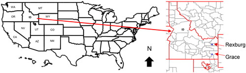
Figure 2. Maps showing the location of sampling points within the (a) Grace and (c) Rexburg fields and elevation for the Grace (b) and Rexburg (d) fields.

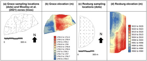
Figure 3. Flow chart summarizing how Sentinel 2 data were selected and NDSI calculated.

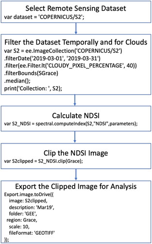
Figure 4. Scree plots for the Grace (a) and Rexburg fields (b,c). Red dashed line shows the optimal number of zones.

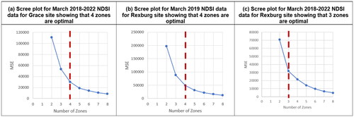
Figure 5. Maps of Key soil and plant variables at the Grace site from different years (a) spring soil moisture 2016, (b) yield 2017, (c) evapotranspiration 2019, (d) crop water productivity 2019, (e) topographic wetness index and (f) aspect.

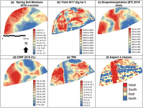
Figure 6. Maps of average rank of NDSI (10m pixels) for (a) January 2017–2022, (b) February 2017–2022, excluding 2020 and (c) March 2020–2022. Low ranks indicate less snow coverage and high ranks more snow coverage.

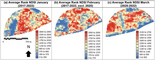
Figure 7. Maps showing location of (a) Woolley et al. zones and (c) 4 class NDSI zones, and Box plots showing the average ranks of March NDSI values for the (b) Woolley et al. zones and (d) the 4 class NDSI zones.

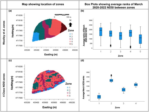
Figure 8. Box plots showing the differences in (a, b) yield 2017 (kg ha⁻¹), (c, d) yield 2018 (kg ha⁻¹), and (e, f) TWI between zones based on the Woolley et al. (2021) classification (a, c, e) and the 4 class NDSI classification (b, d, f).

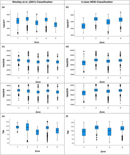
Figure 9. Box plots showing the differences in (a, b) Aspect (degrees), (c, d) Evapotranspiration – ET 2019 (mm) and (e, f) crop water productivity – CWP 2019 (%) between zones based on the Woolley et al. (2021) classification (a, c, e) and the 4 class NDSI classification (b, d, f).

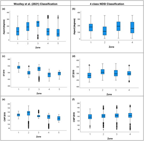
Figure 10. Maps for the Rexburg Site showing (a) March 2019 average rank of NDSI, (b) March 2019 NSDI zones, (c) 2019 wheat yield, (d) average NDSI ranks March 2018–2022, (e) March 2018–2022 NDSI zones and (f) VWC 25 June 2019. Field appears a different shape in different figures because some years the whole field was irrigated and in others, just the inner semi-circle was irrigated. Black lines in (c) show soil series boundaries.

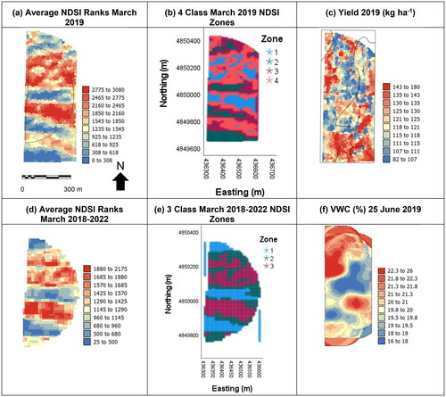
Figure 11. Boxplots for the Rexburg site: Box plots showing the differences in (a) March 2019 NDSI, (c) yield 2019 (kg ha⁻¹) and (e) TWI between zones based on March 2019 NDSI and (b) average March 2018–2022 NDSI, (d) VWC (%) 31 may 2019 and (f) VWC (%) 25 June 2019 based on March 2018–2022 NDSI zones.

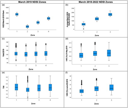
Table 1. Results from Kruskal Wallis H tests comparing the Woolley et al. classification and the 4 class NDSI zones for different variables at the Grace site.

	Woolley et al. zones		4 Class NDSI zones
Variable and date	p-Value	Classes with highest and lowest mean ranks (e.g. H-1, L-5)	p-Value	Classes with highest and lowest mean ranks (e.g. H-1, L-4)
Yield 2017 (wheat)	<0.001	H-2, L-5	<0.001	H-2, L-1
Yield 2018 (potato)	<0.001	H-1, L-3	<0.001	H-2, L-1
TWI	<0.001	H-1, L-3	<0.001	H-2, L-1
Aspect 4 class	<0.001	H-3, L-5	<0.001	H-3, L-2
Spring soil moisture 2016	<0.001	H-1, L-4	<0.001	H-2, L-1
ET 2019	<0.001	H-1, L-4	<0.001	H-2, L-1
CWP 2019	<0.001	H-2, L-5	<0.001	H-4, L-1

Table 2. Results from Kruskal Wallis H tests comparing the March 2019 4 class NDSI classification and the March 2018-2022 3 class NDSI zones for different variables at the Rexburg site.

	4 Class March 2019 NDSI zones		3 Class March 2018–2022 NDSI zones
Variable and date	p-Value	Classes with highest and lowest mean ranks (e.g. H-1, L-4)	p-Value	Classes with highest and lowest mean ranks (e.g. H-1, L-3)
Yield 2019 (wheat)	<0.001	H-1, L-2	<0.001	H-3, L-1
Slope (degrees)	<0.001	H-1, L-3	<0.001	H-3, L-2
TWI	<0.001	H-1, L-2	<0.001	H-2, L-1
Aspect 4 class	<0.001	H-1, L-2	<0.001	H-2, L-3
Average VWC 2019	<0.001	H-1, L-2	<0.001	H-3, L-1
VWC 29 April 2019	0.064	H-4, L-2	<0.001	H-2, L-1
VWC 31 May 2019	0.001	H-4, L-2	<0.001	H-3, L-1
VWC 25 June 2019	<0.001	H-4, L-2	<0.001	H-3, L-1
VWC 29 August 2019	<0.001	H-4, L-2	<0.001	H-3, L-1

References

- Abudu S, Sheng Z, Cui C, Saydi M, Sabzi H, King JP. 2016. Integration of aspect and slope in snowmelt runoff modeling in a mountain watershed. Water Sci Eng. 9(4):265–273. doi: 10.1016/j.wse.2016.07.002.
- Allen RG, Pereira LS, Rae D, Smith M. 1998. Crop evapotranspiration: guidelines for computing crop water requirements. FAO irrigation and drainage paper no. 56. Rome (Italy): Food and Agriculture Organization of the United Nations.
- Blankinship JC, Meadows MW, Lucas RG, Hart SC. 2014. Snowmelt timing alters shallow but not deep soil moisture in the Sierra Nevada. Water Resour Res. 50(2):1448–1456. doi: 10.1002/2013WR014541.
- Choubin B, Alamdarloo EH, Mosavi A, Hosseini FS, Ahmad S, Goodarzi M, Shamshirband S. 2019. Spatiotemporal dynamics assessment of snow cover to infer snowline elevation mobility in the mountainous regions. Cold Regions Sci Technol. 167:102870. doi: 10.1016/j.coldregions.2019.102870.
- Choubin B, Roshan H, Hosseini F, Rahmati O, Melesse AM, Singh VP. 2019. Effects of large-scale climate signals on snow cover in Khersan watershed, Iran. In: Melesse AM, Abtew W, Senay G, editors. Extreme hydology and climate variability. Amsterdam: Elsevier; p. 1–10.
- Choubin B, Solaimani K, Rezanezhad F, Roshan MH, Malekian A, Shamshirband S. 2019. Streamflow regionalization using a similarity approach in ungauged basins: application of the geo-environmental signatures in the Karkheh River Basin, Iran. Catena. 182:104128. doi: 10.1016/j.catena.2019.104128.
- Choubin B, Solaimani K, Roshan MH, Malekian A. 2017. Watershed classification by remote sensing indices: a fuzzy c-means clustering approach. J Mt Sci. 14(10):2053–2063. doi: 10.1007/s11629-017-4357-4.
- Cohen Y, Vellidis G, Campillo C, Liakos V, Graff N, Saranga Y, Snider JL, Casadesús J, Millán S, del H, et al. 2021. Applications of sensing to precision irrigation. In: Kerry R, Escolà A, editors. Sensing approaches for precision agriculture. Cham (Switzerland): Springer Nature; p. 133–157.
- Conrad O, Bechtel B, Bock M, Dietrich H, Fischer E, Gerlitz L, Wehberg J, Wichmann V, Böhner J. 2015. System for Automated Geoscientific Analyses (SAGA) v. 2.1.4. https://gmd.copernicus.org/articles/8/1991/2015/gmd-8-1991-2015.html
- Dozier J, Green RO, Nolin AW, Painter TH. 2009. Interpretation of snow properties from imaging spectrometry. Remote Sens Environ. 113: s 25–S37. doi: 10.1016/j.rse.2007.07.029.
- Drought Monitor. 2023. [accessed 2022 Sep 31]. https://droughtmonitor.unl.edu/.
- Github palettes. 2023. [accessed 2022 Apr 30]. https://github.com/gee-community/ee-palettes/.
- Github spectral indices. 2023. [accessed 2022 Apr 30]. https://github.com/awesome-spectral-indices/awesome-spectral-indices/.
- Hall DK, Riggs GA. 2007. Accuracy assessment of the MODIS snow-cover products. Hydrol Process. 21(12):1534–1547. doi: 10.1002/hyp.6715.
- Hall DK, Riggs GA, Salomonson VV. 1995. Development of methods for mapping global snow cover using Moderate Resolution Imaging Spectroradiometer (MODIS) data. Remote Sens Environ. 54(2):127–140. doi: 10.1016/0034-4257(95)00137-P.
- IBM Corp. 2020. IBM SPSS Statistics for Windows (Version 27.0) [Computer software]. Armonk (NY): IBM Corp.
- IEEE. 2023. [accessed 2023 Jun 5]. https://ieeexplore.ieee.org/document/399618/.
- Jacquez GM, Goovaerts P, Kaufmann A, Rommel R. 2014. SpaceStat 4.0 user manual: software for the space-time analysis of dynamic complex systems, 04/2014. 4th ed. Ann Arbor (MI): BioMedware.
- Khosla R, Inman D, Westfall DG, Reich RM, Frasier M, Mzuku M, Koch B, Hornung A. 2008. A synthesis of multi-disciplinary research in precision agriculture: site-specific management zones in the semi-arid western Great Plains of the USA. Precision Agric. 9(1–2):85–100. doi: 10.1007/s11119-008-9057-1.
- Larson J, Lidberg W, Agren AM, Laudon H. 2022. Predicting soil moisture conditions across a heterogeneous catchment using terrain indices. Hydrol Earth Syst Sci. 26(19):4837–4851. doi: 10.5194/hess-26-4837-2022.
- Lin JT, Feng XZ, Xiao PF, Li H, Wang JG, Li Y. 2012. Comparison of snow indexes in estimating snow cover fraction in a mountainous area in Northwestern China. IEEE Geosci Remote Sens Lett. 9:725–729.
- Mulla DJ. 2021. Satellite remote sensing for precision agriculture. In: Kerry R, Escolà A, editors. Sensing approaches for precision agriculture. Cham (Switzerland): Springer Nature; p. 19–57.
- Nagajothi M, Priya G, Sharma P. 2019. Snow cover estimation of western Himalayas using Sentinel-2 high spatial resolution data. Indian J Ecol. 46:88–93.
- Nyamgerel Y, Jung H, Koh D, Ko K, Lee J. 2022. Variability in soil moisture by natural and artificial snow: a case study in Mt. Balwang area, Gangwon-do, South Korea. Front Earth Sci. 9:786356. doi: 10.3389/feart.2021.786356.
- Oliver MA. 2013. Precision agriculture and geostatistics: how to manage agriculture more exactly. Significance. 10(2):17–22. doi: 10.1111/j.1740-9713.2013.00646.x.
- Oroza CA, Bales RC, Stacy EM, Zheng Z, Glaser SD. 2018. Long-term variability of soil moisture in the southern Sierra: measurement and prediction. Vadose Zone J. 17(1):1–9. doi: 10.2136/vzj2017.10.0178.
- Ortiz BV, Lena BP, Morlin F, Morata G, Duarte de Val M, Prasad R, Gamble A. 2022. Can topographic indices be used for irrigation management zone delineation. Proceedings of the 15th International Conference on Precision Agriculture, Minneapolis, Minnesota, June 2022; p. 26–29.
- O’Shaughnessy SA, Evett SR, Colaizzi PD, Andrade MA, Marek TH, Heeren DM, Lamm FR, LaRue JL. 2019. Identifying advantages and disadvantages of variable rate irrigation: an updated review. Appl Eng Agric. 35(6):837–852. doi: 10.13031/aea.13128.
- Redding T, Devito K. 2011. Aspect and soil textural controls on snowmelt runoff on forested Boreal Plain hillslopes. Hydrol Res. 42(4):250–267. doi: 10.2166/nh.2011.162.
- Riggs GA, Hall DK, Salomonson VV. 1994. A snow index for the Landsat thematic mapper and moderate resolution imaging spectroradiometer. Proceedings of IGARSS '94 - 1994 IEEE International Geoscience and Remote Sensing Symposium, Pasadena, CA, USA, Vol. 4; p. 1942–1944.
- Sharma V, Mishra VD, Joshi PK. 2012. Snow cover variation and streamflow simulation in a snow-fed river basin of the Northwest Himalaya. J Mt Sci. 9(6):853–868. doi: 10.1007/s11629-012-2419-1.
- Shimamura Y, Izumi T, Matsuyama H. 2006. Evaluation of a useful method to identify snow-covered areas under vegetation - comparisons among a newly proposed snow index, normalized difference snow index, and visible reflectance. Int J Remote Sens. 27(21):4867–4884. doi: 10.1080/01431160600639693.
- Smith R, Oyler L, Campbell C, Woolley EA, Hopkins BG, Kerry R, Hansen NC. 2021. A new approach for estimating and delineating within-field crop water stress zones with satellite imagery. Int J Remote Sens. 42:6005–6024.
- Svedin JD, Kerry R, Hansen NC, Hopkins BG. 2021. Identifying within-field spatial and temporal crop water stress to conserve irrigation resources with variable-rate irrigation. Agronomy. 11(7):1377. doi: 10.3390/agronomy11071377.
- Tisseyre B, McBratney AB. 2008. A technical opportunity index based on mathematical morphology for site-specific management: an application to viticulture. Precision Agric. 9(1–2):101–113. doi: 10.1007/s11119-008-9053-5.
- Wiebe K, Gollehon N. 2006. Agricultural resources and environmental indicators, 2006 edition. Economic Information Bulletin No. (EIB-16); p. 239.
- Williams AP, Cook BI, Smerdon JE. 2022. Rapid intensification of the emerging southwestern North American megadrought in 2020–2021. Nat Clim Chang. 12(3):232–234. doi: 10.1038/s41558-022-01290-z.
- Williams CJ, McNamara JP, Chandler DG. 2009. Controls on the temporal and spatial variability of soil moisture in a mountainous landscape: the signature of snow and complex terrain. Hydrol Earth Syst Sci. 13(7):1325–1336. doi: 10.5194/hess-13-1325-2009.
- Woolley EA, Kerry R, Hansen NC, Hopkins BG. 2021. Variable rate irrigation: investigating within zone variability. European Conference of Precision Agriculture, Budapest, Hungary, July 2021; p. 635–641.
- Zhang HB, Zhang F, Zhang GQ, Yan W, Li SE. 2021. Enhanced scaling effects significantly lower the ability of MODIS normalized difference snow index to estimate fractional and binary snow cover on the Tibetan Plateau. J Hydrol. 592:125795. doi: 10.1016/j.jhydrol.2020.125795.