Urban land use land cover classification based on GF-6 satellite imagery and multi-feature optimization

Abstract

Urban land use/land cover (LULC) classification has long been a hotspot for remote sensing applications. With high spatio-temporal resolution and multispectral, the recently launched GF-6 satellite provides ideal open imagery for LULC mapping. In this study, we utilized multitemporal GF-6 images to generate six types of land features, including spectral bands, texture features, built-up, waterbody, vegetation, and red-edge indices. The minimum Redundancy Maximum Relevance (mRMR) algorithm was employed to optimize feature selection. Subsequently, Random Forest (RF) and Extreme Gradient Boosting (XGBT) were assessed using different feature selections. Besides, various feature configurations were designed for LULC classification and comparison. The results indicate that the mRMR-based RF method achieved the highest overall accuracy of 91.37%. The temporal red-edge indices were important features for urban LULC classification and contributed mainly to grassland and cropland. These results supplement existing classification methods and assist in improving LULC mapping in urban areas with complex landscapes.

Keywords:

• GF-6 imagery
• urban land use/land cover
• mRMR
• random Forest
• extreme gradient boosting

1. Introduction

Urbanization is a significant process of human social development. The urbanization process manifests in geospatial terms as the expansion of urban land, and the concentrated population activities and economic development in cities drive the rapid transformation of land use types, forming an urban environment with a complex surface landscape (Fu and Weng 2016; Dadashpoor et al. 2019). Urban land use/land cover (LULC) is the fundamental data for regional urban status monitoring, dynamics development, and planning management (Vadrevu et al. 2019). Remote sensing data is an efficient tool for mapping large-scale and high-precision LULC maps. In the application of remote sensing monitoring, urban LULC classification faces problems such as ‘ecological complexity, phenological diversity, and spectral mixing’ (Cai et al. 2019; Jozdani et al. 2019; Pflugmacher et al. 2019), and there are still challenges in obtaining accurate LULC classification.

To address the challenges faced by urban LULC classification, in previous studies, scholars have carried out this task mainly from multi-source features and classification algorithms. Multi-source features have generally been performed by multi-source images combination (Chen et al. 2017; Zhang et al. 2020), the fusion of special bands (Adelabu et al. 2014), and extraction of remote sensing indices and texture features (Stromann et al. 2019; Yanan et al. 2021), to achieve improved accuracy of LULC classification by enriching surface information (Lv et al. 2014). For classification algorithms to determine the urban land use type, the traditional classification models include the maximum likelihood method (MLC) (Patil et al. 2012), the K-mean mean method, the Iterative Self-organized Data Analysis (ISODATA) (Sharma et al. 2013), and the fuzzy clustering method. In the last decade, machine learning classifiers such as support vector machines (SVM) (Chi et al. 2008), tree-based models (Ghosh et al. 2014; Abdi and Sensing 2020), and neural networks (Zhai et al. 2020) have been widely used in LULC studies and emerged as more accurate and effective solutions than traditional parameterization methods. However, some algorithms require complex parameters and are difficult to automate (Rodriguez-Galiano et al. 2012b). The tree-based models employ ensemble learning approaches, utilizing multi-base classifiers to generate robust classifiers through decision rules or error minimization technique, which attracted a lot of interest due to their ease of use and higher accuracy (Belgiu and Drăguţ 2016; Saini and Ghosh 2019). Random Forest (RF) and Extreme Gradient Boosting (XGBT) are representative tree-based models of bagging and boosting ensemble methods (Breiman 2001; Chen and Guestrin 2016), respectively, and have been used in a wide range of remote sensing classifications. Multiple features are used as input data for the classifier to build classification rules. The number and quality of the input features are related to the classification accuracy, but also to the operation time (Georganos et al. 2018; Zhang et al. 2019). For feature selection, the redundant and invalid features are removed without reducing the important information. Empirical studies have demonstrated that feature selection can strongly influence classification performance in most cases (Eisavi et al. 2015; Rodriguez-Galiano et al. 2012a). Indeed, the random forest embedded feature importance metric that uses out-of-bag (OOB) samples to assess mean decrease accuracy (MDA), and has been applied to feature selection for LULC (Zhang et al. 2019). However, Yang et al. (2017) argue that the MDA metric may be biased and variable. Fortunately, existing research has found that relevance-based feature selection method could achieve the desired classification accuracy using a reduced amount of data (Ma et al. 2017), especially for high-dimensional and redundant features. These characteristics make it more suitable for multi-featured urban cover classification.

In urban surface classification studies, the data sources can be divided into mono-temporal imagery and multi-temporal imagery. Multi-temporal imagery is able to supplement the seasonal change information of classes and assist in land use discrimination (Hütt et al. 2016; Zhao et al. 2016). Senf et al. (2015) found that remote sensing images in spring and autumn are significant for vegetation cover classification. Multi-temporal images compensate for the lack of single-temporal ones. Still, their use is subject to two limitations: it is not easy to obtain high-quality multi-period images (Knight et al. 2006), and high-resolution images are usually not accessible within a short period (Yang et al. 2015).

With the development of remote sensing technology, satellite observation systems have evolved toward high spatial, temporal, and spectral resolution (Houborg and McCabe 2018), of which the Gaofen series satellite independently developed by China is representative. The GF-6 satellite belongs to the optical remote sensing satellite of the Gaofen series, launched in June 2018, with the high spatial and temporal resolution, multi-spectrum, and wide-width imaging (Zhang et al. 2021). Its multispectral imagery has eight spectral bands, four bands as the GF-1 satellite image, two red-edge bands, a yellow band, and a purple band, and is freely available. The satellite revisit cycle is four days. High spatio-temporal resolution and multispectral imagery can provide sufficient and practical information for urban surface coverage classification. At present, studies on GF-6 have been carried out to assess its potential for agricultural landscape mapping (Xia et al. 2022). However, there are presently no studies that are evaluating the performance of LULC classification of GF-6 satellite images in complex urban landscapes. Based on the data advantages of GF-6 imagery, the classification method of long-time series images and multiple features using GF-6 data is worth exploring.

In order to address the challenge of accurately classifying complex urban land use, this study utilizes the time-series data from GF-6 MFV as the data source. A comprehensive feature set comprising various types of features, including band features, spectral index features, red-edge features, and texture features, is extracted from GF-6 data. The mRMR algorithm is employed for feature selection. Two robust tree classifiers, RF and XGBT, are evaluated using different sets of selected features. Additionally, the study explores the potential of different types of feature combinations in LULC classification. The findings of this research pinpoint the optimal classification scheme using GF-6 images, serving as a valuable reference for achieving high accuracy in LULC monitoring.

2. Study area and data

2.1. Study area

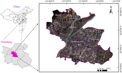
Nanchang, the capital of Jiangxi Province, is one of the central cities in the Yangtze River metropolitan area (Zhang and Xu 2015). It is located between 115°49′-116°3′E and 28°34′-28°48′N, and has a subtropical monsoon climate with abundant rain and heat. The primary urban districts, including Xihu, Donghu, Qingyunpu, and Qingshanhuqu, was chosen as study area (Figure 1). It has a slight slope from the northeast to the southwest, with a dense water network. Besides, Nanchang is known as the ‘land of fish and rice’ because of its well-developed agriculture (Zheng and Qingyun 2021). As a built-up area, the study area is complex in terms of landform characteristics, with various landforms interspersed. According to the actual situation of land cover in the study area, and referring to the widely adopted classification scheme (Brewster et al. 1999) for land use in remote sensing, the types of LULC in this study were classified into six types: forestland, grassland, cropland, built-up land, unused land, and water.

Figure 1. Location of study area, with true colour composite map illustrating full extent of the study area.

2.2. Data

GF-6 Satellite is a low-orbit optical imaging remote sensing satellite. It carries a high-resolution camera (PMS) and a multispectral wide-format camera (MFV). The MFV sensor innovatively realizes the Chinese CMOS detection of 8-band multispectral products (Xia et al. 2022). The bands of GF-6 are expanded to 8, for which band 1-4 are similar as GF-1 and GF-2, and band5-8 are added bands, including two red-edge bands, one yellow band and one purple band. In this study, time series MFV images were used for urban land use classification. The spectral band information of the GF-6 MFV images is shown in Table 1.

Table 1. Spectral bands of the GF-6 satellite.

Band name	Bandwidth (μm)	Spatial resolution (m)
Band 1 Blue	0.45 ∼ 0.52	16
Band 2 Green	0.52 ∼ 0.59	16
Band 3 Red	0.63 ∼ 0.69	16
Band 4 NIR	0.77 ∼ 0.89	16
Band 5 Red edge1	0.69 ∼ 0.73	16
Band 6 Red edge2	0.73 ∼ 0.77	16
Band 7 Purple	0.40 ∼ 0.45	16
Band 8 Yellow	0.59 ∼ 0.63	16

We obtained all GF-6 images from the National Resource Satellite Application Platform (http://www.cresda.com). To obtain more information about the phenological changes, we collected six MFV images with acquisition dates corresponding to 19 February 2021, 30 April 2021, 31 August 2021, 28 September 2021, 25 November 2021, and 19 December 2021. They contain seasonal information on the four seasons: spring, summer, autumn, and winter. Radiometric calibration, atmospheric correction, and orthorectification were addressed in the time-serious images using the ENV 5.3 platform. In addition, geographic alignment was performed with Automated and Robust Open-Source Image Co-Registration Software (AROSICS) to match the spatial positions of the different images, and the special error was validated within 1 pixel (Scheffler et al. 2017). We obtained administrative boundary data from the National Geomatics Center of China (http://www.ngcc.cn/ngcc/).

2.3. Training and testing samples

It is commonly believed that sample quality could directly affect the accuracy of classification results, so representative pixels should be selected (Liu et al. 2017). To collect training samples, we collected 110 small polygons for each LULC class and obtained several relatively homogenous pixels in each polygon. Training samples cover the gradient and diversity of land use types, such as low/high density vegetation and different built area, in order to reduce the impact of spatial autocorrelation. For testing samples, 250 points for each LULC type were randomly selected. To ensure independence between training samples and testing points, the closest testing points was located at least 50 meters away from the training polygon. In this study, samples were marked from the time series of GF-6 MFV images and Google Earth history high-resolution images by visual interpretation. After that, samples were checked against the land use distributing map of Nanchang City in 2020. All labelled samples were further examined by co-authors before modelling. As result, 658 training polygons and 1472 testing points were obtained. Specifically, the testing sample sizes for each category are as follows: forestland (247 samples), grassland (236 samples), cropland (246 samples), built-up land (250 samples), unused land (243 samples), and water (250 samples).

3. Method

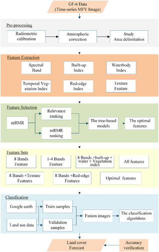
Choosing enough features for data classification is very important, as it can provide as much as possible effective information of different kinds of objects for identifying them. In this study, we combined bands features, index features and texture features to find optimal feature sets for classification. Within it, red-edge index features are calculated with red-edge bands, as band 5 and 6 of GF-6. We used multi-temporal GF-6 images for urban LULC classification to create time-series vegetation indices, with the image from April 30, 2021 as the main image. First, six GF-6 images are taken to build multiple features. Second, all these features are optimized with the mRMR algorithm to downscale features, meanwhile, two well-known tree machine learning models, RF and XGBT, are used to compare the impact of different feature configurations. Third, seven feature sets are developed to assess the impact of different feature types on urban LULC classification. Finally, the classification algorithms are trained and evaluated on different sets of classification features and the suitable set is explored to improve LULC classification. The main process is shown in Figure 2.

Figure 2. The overall framework of the urban land use/land cover classifications using GF-6 imagery.

3.1. Feature variable set

Spectral bands are the pixel values of different objects generated by the sensor receiving electromagnetic waves reflected from the ground. Usually, ground objects do not differ significantly in terms of individual band information, and index features are able to emphasize the differences among ground objects through band calculation (Yang et al. 2014). In addition, texture features measure the relationship between multiple pixels within an area. The texture features obtained from the grayscale co-occurrence matrix are statistical pixel values in the local image information, that reflect the distribution and variation of pixels with their spatial neighbourhoods, and can attenuate the ‘same spectrum and different objects’ or ‘same object and different spectrum’ caused by ‘misleading’ (Hall-Beyer 2017). In order to fully exploit the heterogeneity characteristics of different ground objects, we selected these six types of features: spectral bands, built-up index, vegetation index, water body index, red-edge index, and texture features according to the land-cover variables based on the GF-6 images.

Spectral bands refer to the GF-6 WFV image. The original image includes blue, green, red, near-infrared, red edge 1, red edge 2, purple and yellow bands, a total of 8 band features.

Using the spectral bands of the original image, this study extracted the built-up index, vegetation index, water body index, and red edge index to gain information between different ground objects. The Built-up index (BAI) has good performance in the surface detection of concrete and asphalt, and is a reflection index of construction land (Shao et al. 2016). The vegetation index includes four indicators: normalized vegetation index (NDVI) (Carlson and Ripley 1997), ratio vegetation index (RVI) (Duveiller et al. 2011), soil adjustment index (SAVI) (Huete 1988) and enhanced vegetation index (EVI) (Ahamed et al. 2011). The commonly used normalized difference water index (NDWI) (Gao 1996), mixed water index (CIWI) (Zhang et al. 2018), and simple ratio water index (SRWI) (Zarco-Tejada et al. 2003) were calculated as water index. The red-edge band has advantages in the accurate monitoring of vegetation. The normalized differential red-edge index (NDre) (Zhang et al. 2019) was calculated to enhance the information of the red-edge band. The normalized red-edge vegetation index (NDVIre) (Ehammer et al. 2010) is an improved vegetation index that employs the red-edge band instead of the near-infrared band.

We used the grey co-occurrence matrix to extract texture features. Due to the consistency of the ground objects’ texture in the same study area, PCA transformation was performed on the main image, and the first two principal components images were extracted to calculate the eight commonly used statistical texture indicators in GLDM, respectively mean, contrast, variance, entropy, homogeneity, second moment, autocorrelation, and dissimilarity. Referring to Zhang’s proposal that 7 × 7 was a suitable window size for texture extraction from medium resolution images (Zhang et al. 2014), this study selects four window sizes of 3, 5, 7, and 9 for comparative experiments. The results show that the window size of 5 × 5 can extract more texture information from GF-6 images, the step size was set to 1, and the grey level to 64.

Studies have shown that NDVI exhibits regularity in the vegetation growth cycle, and NDVIre has high sensitivity in vegetation identification (Wang et al. 2008). Since seasonal difference is an essential characteristic of vegetation, we used multiple images to construct the time series of NDVI and NDVIre as seasonal features. Taking the GF-6 image on April 30, 2021 as the main data, a total of 8 spectral bands, 26 index features and 16 texture features were calculated as the feature sets for surface coverage classification. The feature list is shown in Table 2.

Table 2. Features extracted from GF-6 images.

Feature serial number	Feature variable	Feature description	Abbreviation of features
1 ∼ 8	Blue Band、 Green Band、Red Band、 Near infrared band、 Rededge_1 Band、 Rededge_2 Band、 Yellow Band、Purple Band	Spectral bands of GF-6 WFV image	Blue, Green, Red, Nir, Rededge1, Rededge2, Yellow, Purple
9	$\mathit{BAI}=(\mathit{blue}-\mathit{NIR})/(\mathit{blue}+\mathit{NIR})$ (Shao et al. 2016)	Built-up index	BAI
10 ∼ 15	$\mathit{NDVI}=(\mathit{NIR}-\mathit{red})/(\mathit{NIR}+\mathit{red})$ (Carlson and Ripley 1997)	Vegetation index	NDVI1 ∼NDVI6
16	$\mathit{SAVI}=(1+L)(\mathit{NIR}-\mathit{red})/(\mathit{NIR}+\mathit{red}+L)$ (Huete 1988)		SAVI
17	$\mathit{EVI}=2.5\frac{(\mathit{NIR}-\mathit{red})}{\mathit{NIR}+6red-7.5b\mathit{lue}+1}$ (Ahamed et al. 2011)		EVI
18	$\mathit{RVI}=\mathit{NIR}/\mathit{red}$ (Duveiller et al. 2011)		RVI
19	$\mathit{NDWI}=(\mathit{green}-\mathit{NIR})/(\mathit{green}+\mathit{NIR})$ (Gao 1996)	Water index	NDWI
20	$\mathit{CIWI}=\mathit{NDVI}+\mathit{nir}$ (Zhang et al. 2018)		CIWI
21	$\mathit{SRWI}=\mathit{Green}/\mathit{NIR}$ (Zarco-Tejada et al. 2003)		SRWI
22 ∼ 33	$\mathit{NDVIre}=(\mathit{NIR}-re{d}_{\mathit{ged}})/(\mathit{NIR}+re{d}_{\mathit{ged}})$ (Zhang et al. 2019)	Red-edge index	NDVIre1_1 ∼NDVIre1_6, NDVIre2_1 ∼NDVIre2_6,
34	$N{D}_{re}=(re{d}_{\mathit{ged}1}-re{d}_{\mathit{ged}2})/(re{d}_{\mathit{ged}1}+re{d}_{\mathit{ged}2})$ (Ehammer et al. 2010)		NDre
36 ∼ 50	Mean、Contrast、Variance、 Entropy 、Homogeneity、 Second Moment 、Correlation、Dissimilarity	Grey level co-occurrence matrix index calculated by the first two principal components	PC1MEAN, PC1V, PC1E, PC1CON, PC1HOM, PC1SEC, PC1COR, PC1DIS, PC2MEAN, PC2V, PC2E, PC2CON, PC2HOM, PC2SEC, PC2COR, PC2DIS

3.2. Feature selection

The abundant image features are conducive to a more comprehensive description of the ground object, but numerous classification features increase the computational complexity and reduce the efficiency of the classifier (Georganos et al. 2018). Among them, the features that contribute little to the classification result could become noise and reduce the classifier accuracy. The purpose of feature selection is to extract practical features for classification from numerous classification features and remove redundant features. The max-relevance min-redundancy (mRMR) algorithm presented by Peng et al. (2005), a filter-type feature selection algorithm, measures the relevance and redundancy of features by calculating the mutual information. The mRMR algorithm specifies two cost functions of information difference (Eq. (1)(1) $${G=\mathrm{m}ax}_{i\in s}\left[I\left(i,\mathrm{ }h\right)-\frac{1}{\left|S\right|}{\sum }_{j\in S}I(i,\mathrm{ }h)\right]$$(1) ) and information entropy (Eq. (2)(2) $$\mathit{Ent}=\mathrm{ }{\max }_{i\in s}\left[I\left(i,\mathrm{ }h\right)/\frac{1}{\left|S\right|}{\sum }_{j\in S}I(i,\mathrm{ }h)\right]$$(2) ), whereupon the information gain of features and target variables is derived to evaluate the relevance. The redundancy is obtained from the dependency degree between the features. Subsequently, the features are ranked according to their scores. The goal of feature selection is to obtain a set of optimal feature subsets with maximum correlation and redundancy removal. The maximum correlation and minimum redundancy are calculated according to Eqs. (3)(3) $$\mathit{maxD}\left(S,\mathrm{ }c\right),\mathrm{ }D=\frac{1}{\left|S\right|}{\sum }_{i=1}^{S}I\left(x_i,\mathrm{ }c\right)$$(3) and (4)(4) $$\mathit{minR}\left(S,c\right),R=\frac{1}{{\left|S\right|}^2}{\sum }_{i=1}^{S}I\left(x_i,\mathrm{ }{x}_j\right)$$(4) , respectively.

1. Information gain and information entropy (1) $${G=\mathrm{m}ax}_{i\in s}\left[I\left(i,\mathrm{ }h\right)-\frac{1}{\left|S\right|}{\sum }_{j\in S}I(i,\mathrm{ }h)\right]$$(1) (2) $$\mathit{Ent}=\mathrm{ }{\max }_{i\in s}\left[I\left(i,\mathrm{ }h\right)/\frac{1}{\left|S\right|}{\sum }_{j\in S}I(i,\mathrm{ }h)\right]$$(2)

2. Maximum correlation (3) $$\mathit{maxD}\left(S,\mathrm{ }c\right),\mathrm{ }D=\frac{1}{\left|S\right|}{\sum }_{i=1}^{S}I\left(x_i,\mathrm{ }c\right)$$(3)

3. Minimal redundancy (4) $$\mathit{minR}\left(S,c\right),R=\frac{1}{{\left|S\right|}^2}{\sum }_{i=1}^{S}I\left(x_i,\mathrm{ }{x}_j\right)$$(4)

Among them, $I(i,\mathrm{ }h)$ is the mutual information of the feature $i$ and the feature $h,$ $S$ is the feature subset, $x_i$ is the i-th feature, and $c$ is the categorical variable. The incremental search method is used to determine the optimal solution of feature comprehensive evaluation operator $\phi (D,\mathrm{ }R),$ that is, assuming that Sm-1 is the acquired feature subset, then find the maximum value of $\phi (D,\mathrm{ }R)$ in the remaining N-Sm-1 features, and select as a new feature.

3.3. Classification schemes

We use the optimal feature set selected with mRMR method as one classification sample set, also design six other classification sample sets to compare classification effects with each other. The objectives of the classification schemes in this study cover three aspects: 1) to analyse the classification contribution of the additional spectral bands of the GF-6 MFV imagery compared with the 4-band data, 2) to compare the effects of different feature types on the extraction of urban LULC from the GF-6 satellite images, and 3) to select best feature sets to develop an urban LULC classification method from the GF-6 MFV images. Therefore, using the feature sets of GF-6 images, seven feature schemes were established as shown in Table 3 for classification tests. The results were evaluated based on confusion matrix. Overall accuracy (OA), Kappa coefficient, producer’s accuracy (PA) and user’s accuracy (UA) are accuracy evaluation metrics.

Table 3. Experimental schemes for seven feature sets.

Classification scheme	Feature set	Feature serial number
Scheme 1	Spectral feature (all bands)	1 ∼ 8
Scheme 2	Spectral feature (band1 – band 4)	1 ∼ 4
Scheme 3	Spectrum + built-up + water + Vegetation index	1 ∼ 8, 9 ∼ 21
Scheme 4	Spectrum + texture	1 ∼ 8, 35 ∼ 50
Scheme 5	Spectrum + Red edge index	1 ∼ 8, 22 ∼ 24
Scheme 6	Spectrum + index + texture	1 ∼ 50
Scheme 7	optimal feature	2, 4, 5, 6, 7, 8, 9, 10, 12, 13, 14, 17, 18, 22, 24, 26, 27, 29, 36

3.4. Classification algorithms

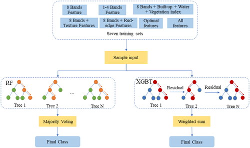
In this study, two tree-based machine learning models are used for classification, RF and XGBT. RF is a non-parametric bagging ensemble algorithm, which is one of the most recognized excellent models in LULC classification using remote sensing data. XGBoost is a relatively new boosting algorithm combined with gradient descent optimization, and it stands out in the field of machine learning due to its robust performance in massive data. In contrast to deep learning models, tree-based models possess certain distinct advantages in low computation cost and stable feature learning ability (Abdi and Sensing 2020).

1. Random Forest

   Random forest consists of the decision tree as the basic unit, and uses the random subspace method to extract samples. The random samples are trained to construct the mapping relationship between features of the sample and targets, and then multiple decision trees are obtained. This helps to reduce the overfitting. After that, the decision trees are assembled through the bagging method, and the classification results are selected by voting.

2. Extreme Gradient Boosting

   XGBT initially works by fitting a decision tree as a base model. Different from the random forest, the samples are trained iteratively in boosting, where each predictor corrects the residual errors made by its predecessor. The gradient descent optimization is employed to build the additive model by using a specified loss function. The XGBT also incorporates parallel techniques to support the speed and accuracy of the process. The final prediction of the model is obtained by weighted summation of each decision tree, and the weights are estimated from the decision tree performance.

   In this study, RF and XGBT implemented with Scikit-Learn, which involves some adjustable parameters. In RF, the number of decision trees (Ntree) and the number of extracted features in node splitting (Mtry) are the two most important parameters. Rodriguez-Galiano et al. (2012b) suggested that Mtry be equal to the arithmetic square root of the number of features. The most important parameters of XGBT are the number of iterations (nrounds), the maximum depth of trees (depth), subsample ratio of the training instance (subsample), and regularization parameters (gamma). The tree-based models usually preform stability when the number of trees or the number of iterations is above 100 (Samat et al. 2020). In this study, grid search is performed using 5-fold cross-validation, and the optimal models are obtained by selecting the best hyperparameters among the pre-selected parameters (Figure 3).

Figure 3. The classification process for Random Forests and Extreme Gradient Boosting.

4. Results

4.1. Features selection and classifier comparison

There were two kinds of features importance ranking provided by the mRMR algorithm, one evaluates the relevance between target and variables, and the other method combines the redundancy between variables. In this study, we calculated the variation in classification accuracy for the selected feature type and number using both feature selection methods in RF and XGBT classifiers, respectively.

To reduce the computational effort of solving the probability function for high-dimensional features, 50 features were discretized by equal frequency intervals in mRMR algorithm. Then computed max-relevance score and max-relevance and min-redundancy score (mRMR score) were obtained. The scores are plotted as two histograms (Figures 4 and 5), with the order of features on the horizontal axis indicating the order of relevance and the order of features selection, respectively.

Figure 4. Relevance ranking based on mRMR algorithm. The horizontal axis represents the feature name. The vertical axis represents the relevance score of each feature.

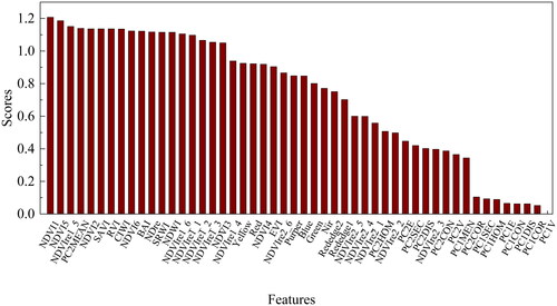
Figure 5. Max-relevance and min-redundancy ranking based on mRMR algorithm. The horizontal axis represents the feature name. The vertical axis represents the mRMR score of each feature.

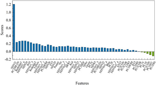
As seen in Figure 4, NDVI1 were the most relevant variables, with a score of 1.2. PC1COR and PC1V had a low correlation with values less than 0.018. Among the 20 most relevant variables, seven variables were red-edge features. According to the mRMR ranking, NDVI1, PC2MEAN, and Rededge1 contribute significantly to urban LULC classification. Then, variables were added one by one to the two tree-based models according to mRMR ranking and Relevance ranking, respectively. The OA and Kappa coefficient were then calculated to identify the relationship between feature configuration and accuracy (Figure 6).

Figure 6. Relationship between number of features, OA and Kappa based on max-relevance and min-redundancy ranking for the two tree-based classifier.

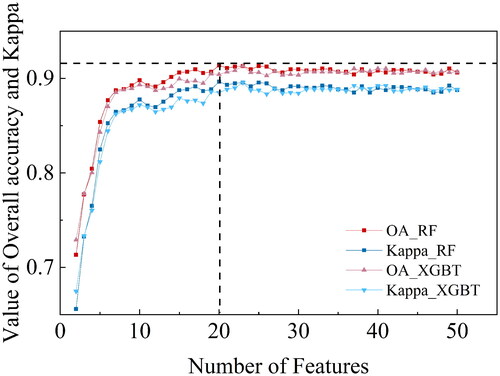
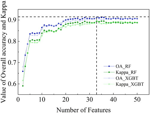
Based on the mRMR ranking, when the number of features grows gradually in the first stage (the number of features < 7), the classification accuracy of both RF and XGBT improves rapidly. Then, as the number of features continues to increase, RF outperforms XGBT, and when the number of features equals 20, RF reaches the highest classification accuracy of 91.37 and Kappa equals 0.90. The best accuracy of XGBT appears to be more RF lagged with an input feature of 23, and the OA and Kappa are 91.30, 0.90, respectively. With the further increase in the number of features, RF and XGBT performed consistently, with a certain decrease in classification accuracy, followed by stabilization. In addition, as for the relevance score (Figure 7), The accuracy trends of both algorithms are similar to the former, but with a slow growth trend. RF and XGBT reached the highest OA value of 91% when the first 33 features of the relevance ranking were input.

Figure 7. Relationship between number of features, OA and Kappa based on relevance ranking for the two tree-based classifier.

The results show that employing the mRMR feature selection method is advantageous for both RF and XGBT classifiers, achieving higher accuracy with a small subset of features. Notably, RF outperformed XGBT by attaining the highest overall accuracy (OA) with a reduced feature set of 20. However, as the number of features increased, XGBT demonstrated comparable stability to RF. In this study, the top 20 features in the mRMR ranking were selected as the optimal feature set to extract the urban LULC classification.

4.2. Accuracy of different classification schemes

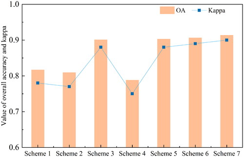
Due to the outstanding and stable performance of RF, it is employed to classify feature fusion images from seven schemes (Figure 8). Figure 9 shows the overall accuracy and Kappa coefficient of the seven feature schemes. Scheme 1 achieved a moderate level of LULC classification accuracy (OA = 81.86%) by solely utilizing the original bands of GF-6. This performance was marginally superior to scheme 2 (OA = 80.91%), which relied on the first four bands of GF-6 (analogous to the 4-band of GF-1 images). Notably, the inclusion of spectral indices or red-edge indices resulted in a significant OA improvement of 8.22% and 8.43% for Scheme 3 and Scheme 5, respectively, yielding overall accuracies of 90.08% and 90.29%. In contrast, Scheme 4 exhibited the lowest OA and Kappa. The OA was reduced by 3.06% compared to the original image classification. Scheme 6, incorporating all available features, achieved an OA of 90.63%. Among all the feature schemes, Scheme 7 based on the selected optimal features, performed with the highest overall accuracy (OA = 91.37%). The above results suggest that our optimal features, which were selected from original bands, band index, texture, and time-series vegetation index by mRMR, better complement information to distinguish the urban LULC categories.

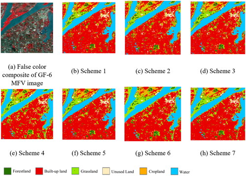
Figure 8. Classification results of seven feature schemes; the black rectangle is area 1, the black ellipse is area 2.

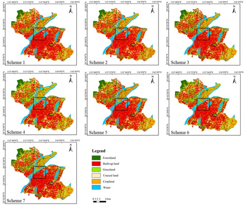
Figure 9. Comparisons of overall accuracy and Kappa derived from RF in different feature schemes.

4.3. Comparison of different classification schemes

We evaluated the image classification results of seven feature sets through both visual interpretation and quantitative evaluation.

To present the classification details, LULC map was zoomed in Area1 (Figure 10), which contains six feature types. There was obvious misclassification among different features in Scheme 1 and Scheme 2, especially in cropland, grassland, and built-up land. Scheme 4 added GLCM texture; the boundaries of various land features became distinct. However, with the exception of water bodies, the other five categories of features were seriously confused. The classification outcomes of Scheme 3 and Scheme 5 exhibit relatively consistent alignment with the reference images. Additionally, there was a distinct advantage over Scheme 1, Scheme 2, and Scheme 4 in terms of distinguishing between different types of vegetation, which are obvious in Area 2 (a park area). Schemes 6 and 7 had the most effective visual classification, characterized by coherent classes and minimal speckling.

Figure 10. Detailed classification results of seven schemes in area 1.

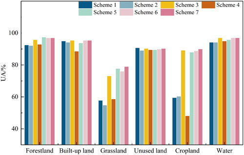
The PA and UA for each category of these seven schemes are shown in Figures 11 and 12. The four additional bands of GF-6 MFV images (Scheme 1) improved the PA and UA on unused land and grassland compared with Scheme 2. Compared to the original image, the utilization of ground object indices (Scheme 3) and the red-edge indices (Scheme 5) resulted in a significant improvement in the UA for various vegetation categories (4.97%-29.67%). Also, the incorporation of ground object indices enhanced the classification accuracy for built-up land and water bodies. Among all the schemes, Scheme 5 exhibited the highest producer’s accuracy (PA) for cropland. Similar with the results presented in Figure 9, Scheme 4 produced the lowest PA in various land types (except forestland). In Scheme 6, which encompassed all features, the classification accuracy (both PA and UA) for grassland, unused land, and cropland was comparatively lower than that of Scheme 7. This indicates that all features have an impact on the classification accuracy. The classification results obtained using the optimal features (Scheme 7) exhibit that PA and UA were ranked highly in each category. Specifically, these results ranked in the top two of the seven schemes evaluated, also with good agreement.

Figure 11. The producer’s accuracy of different categories in 7 schemes.

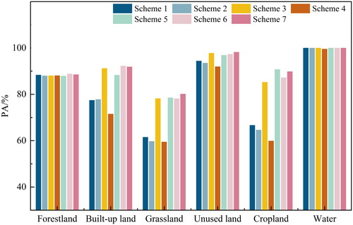
Figure 12. The User’s accuracy of different categories in 7 schemes.

4.4. Performance assessment of the multi-feature optimization classification

Table 4 shows the confusion matrix of multi-feature optimization classification based on GF-6 MFV imagery. Among all land types, the water and unused land were the top two with PA equal to 100% and 98.21%, respectively. Built-up land achieved the ideal classification results, with both PA and UA of more than 90%. The forestland was also accurate in terms of the PA and UA (88.52% and 96.76%, respectively). Compared to forestland, grassland was not in good consistency with validation data. The PA and UA for grassland were 80.17% and 78.81%, respectively. The confusion between forestland and grassland in the city is a problematic aspect of the land-cover classification, which is related to their complex surface distribution in the urban area. In this study, the confusion between forestland and grassland was controlled at 7.41%, which is a relatively desirable value. The PA and UA for cropland were in consistent equal to 89.84%. The temporal vegetation index (the red edge index included) could considerably extract cropland.

Table 4. Confusion matrix of the classification results using the optimal features.

Class	Ground truth
	F	B	G	U	C	W	Total	UA(%)
F	239	1	7	0	0	0	247	96.76
B	0	238	7	4	1	0	250	95.2
G	27	2	186	0	21	0	236	78.81
U	0	12	10	219	2	0	243	90.12
C	4	2	19	0	221	0	246	89.84
W	0	4	3	0	1	242	250	96.8
Total	270	259	232	223	246	242
PA (%)	88.52	91.89	80.17	98.21	89.84	100
OA= 91.37% Kappa = 0.90

Note: F – Forestland, B – Built-up land, G – Grassland, U – Unused land, C – Cropland, W – Water.

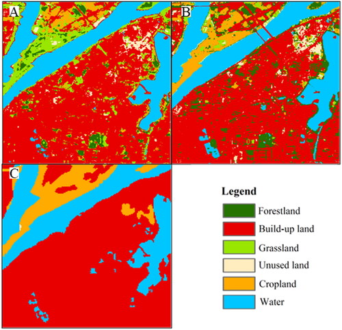
We also compared our classification with the ESA WorldCover (Zanaga et al. 2022) and GlobeLand30 (Jun et al. 2014). These two classified products of the study area, produced in 2021 and 2020 with a resolution of 10 m and 30 m respectively, were used as samples. To ensure a meaningful and fair comparison, it was necessary to account for the varying LULC categories of the different products. Among the three products, we focused on six land categories in this study that were common and comparable. While, ‘wetland’ category was not included in the comparison due to its limited extent. Figure 13 shows the selected sub-region in three products (same place with Figure 10). The complete LULC maps of the study area was shown in Appendix B. And the confusion between cropland and grassland poses a significant challenge in the LULC classification (Schulz et al. 2021). Therefore, it is understandable that there are distinctions between these two land types across various datasets. Comparison with GlobeLand30 reveals that both ESA WorldCover and our multi-feature optimization method performed better in the details of urban LULC classification. When examining the riverbank area, ESA WorldCover and GlobeLand30 have classified it primarily as agricultural land, whereas our findings primarily mapped natural vegetation. A likely reason for this phenomenon is that grassland or cropland along the braided bars of rivers is more sensitive to seasonal changes. Regarding the built-up portion of the subregion, ESA WorldCover tends to overestimate cropland, and there is also confusion between construction land and bare soil. As for our results, a limitation is that the interface between vegetation and buildings is often interpreted as grassland. In addition, the OA of the different classification results was computed, with multi-feature optimization classification ranked first in the accuracy among the three classifications, followed by ESA WorldCover and GlobeLand30, with accuracies of 77.16% and 53% respectively.

Figure 13. A comparison of LULC classifications among (a) our proposed method, (b) the ESA WorldCover, and (c) GlobeLand30.

5. Discussion

Accurate land use is crucial for numerous applications, but effectively mapping complex urban landscapes remains serious challenges. However, with the advent of diverse remote sensing technologies, there are now valuable opportunities to achieve large-scale and highly accurate urban LULC mapping. In this study, we used time-series GF-6 MFV images to extract multiple indices and grayscale co-occurrence matrices to capture the spectral and texture variations of various features. And a total of 50 features were created. Subsequently, mRMR performed two types of feature selection. And we employed two tree-based models and combined different input features to evaluate their classification accuracy. Finally, we fused various types of feature combinations for mapping to compare their performance in urban LULC classification.

Our results demonstrate that both RF and XGBT can enhance model performance when using reduced features under optimal parameter selection, which supports the finding of Belgiu and Drăguţ (2016) that eliminating redundant features is significant for LULC classification. Comparing the two feature selection methods, we found that the minimum redundancy maximum relevance feature selection requires fewer features than the correlation-based feature selection to achieve the highest accuracy. Incorporating the mutual information between features and feature-target can extract features more efficiently thus enhancing sample reliability and make classification, which further validates the findings of Kiala et al. (2019). In this study, the mRMR-based RF classifier was the superior model, using only 20 variables to achieve higher classification accuracy. While, XGBT exhibited lower performance than RF when fewer features were employed. Both models showed some degradation in performance but maintained at a certain level when all features are processed, which is consistent with the theory that tree-based models are less prone to overfitting (Georganos et al. 2018; Schulz et al. 2021).

Based on the feature importance of mRMR, the four new added bands of GF-6, particularly the two red-edge bands, exhibited a strong ability to distinguish LULC. In comparison to the purple and yellow bands, the red-edge bands contain more information for classifying LULC (Saini and Ghosh 2019). Furthermore, in the classification results with various feature types, it was observed that the four additional bands enhance the accuracy of identifying grassland and bare land. Additionally, the utilization of ground object indices proves beneficial in effectively distinguishing different land types. Moreover, the red-edge features derived from the time series exhibit remarkable capability in classifying different vegetation and enhancing the classification of other features. However, it is important to note that not all features can contribute to the LULC classification (Bai et al. 2021). In this study, the redundant texture features introduced the interference in the LULC classification process. These findings corroborate previous research (Hütt et al. 2016; Stromann et al. 2019; Schulz et al. 2021), underscoring the importance of considering feature diversity and temporal variation for achieving favourable results in LULC classification.

The combination of GF-6 images and feature optimization showed significant potential for accurately mapping LULC in urban areas, with an overall accuracy of 91.37%. Specifically, our LULC mapping results exhibit high classification accuracy for built-up land, unused land, and water bodies, all exceeding 90%. Meanwhile, it shows consistent and accurate mapping on cropland. This result indicates that the GF-6 images stand out in identifying various phenological characteristics of agricultural crops, aligning with the observations made by Xia et al. (2022). However, the accuracy of grassland was comparatively lower, and the confusion between grassland and forest land is high, probably due to the random scattered distribution of dense or sparse vegetation in urban areas (Guo et al. 2011; Kowe et al. 2020).

Although our findings offer valuable insights into the classification of urban LULC using GF-6 images, there are certain limitations that need to be addressed. Firstly, the LULC types used in this study are limited in scope. It would be worthwhile to further explore the classification potential of the proposed classification method and the GF-6 feature set across a broader range of LULC types. Additionally, future studies should consider incorporating other comparable satellite observations such as Landsat 8 and Sentinel-2. By comparing different data sources and investigating the synergy between these sources and GF-6 data, the classification accuracy of urban LULCs can be further enhanced.

6. Conclusions

The GF-6 MFV sensor offers a publicly accessible data source that consists of high-resolution images with both spatial and temporal precision. It includes additional two red-edge bands, purple and yellow band, and provides imagery with a temporal resolution of 4 days. This study focuses on investigating the capabilities of GF-6 imagery for urban LULC mapping. We developed a feature filtering classification framework that involves extracting multi-temporal image features. To identify the most informative features, we employed the minimum Redundancy Maximum Relevance (mRMR) algorithm to generate subsets of these features, combined with two robust classifiers, RF and XGBT, for classification task. The various feature configurations were compared to assess their performance on LULC classification.

Our results indicate that the inclusion of more features does not necessarily lead to an improvement in the accuracy of LULC classification. By utilizing mutual information, the mRMR method effectively selects features, consequently enhancing the classification performance of RF and XGBT. The characteristics of GF-6 for LULC classification show improvements in various aspects. Firstly, in terms of bands, the four new bands of GF-6 MFV can contributes to reducing the confusion problem of vegetation and bare land. Secondly, temporal features. The utilization of spectral indices across multiple time series windows is a key to accurate LULC classification. In particular, the inclusion of temporal red-edge features can prove valuable in distinguishing different feature classes. The evaluation of the LULC classification based on mRMR and GF-6 images exhibit an overall accuracy of 91.34%. And most of the feature classes have PA and UA above 85%. These results affirm the significant potential of GF-6 imagery for LULC classification in complex and diverse urban areas.

Authors contribution

Xiaobing Wei: Conceptualization, Data curation, Methodology, Validation, Writing – original draft. Wen Zhang: Conceptualization, Methodology, Formal analysis, Writing – review & editing. Zhen Zhang: Resources, Data curation, Writing – review & editing. Haosheng Huang: Resources, Supervision, Writing – review & editing. Lingkui Meng: Conceptualization, Resources, Supervision.

Data availability statement

The data that support the findings of this study are available from the corresponding author, WZ, upon reasonable request.

Disclosure statement

No potential conflict of interest was reported by the authors.

Correction Statement

This article has been corrected with minor changes. These changes do not impact the academic content of the article.

Additional information

Funding

This research was supported by the National Key Research and Development Program of China (No.2021YFB3900603), and the China Scholarship Council (No. 202106270030).

Appendix A.

The producer’s accuracy and user’s accuracy of different categories in 7 feature set schemes

Table

Scheme	type	PA	UA
Scheme 1	Forestland	88.37%	92.3%
	Built-up land	77.45%	94.8%
	Grassland	61.53%	57.63%
	Unused land	94.42%	90.53%
	Cropland	66.67%	59.35%
	water	100%	94%
Scheme 2	Forestland	87.98%	91.9%
	Built-up land	77.81%	94%
	Grassland	59.72%	54.66%
	Unused land	93.51%	88.89%
	Cropland	64.63%	60.16%
	water	100%	94%
Scheme 3	Forestland	88.05%	95.54%
	Built-up land	91.19%	95.2%
	Grassland	78.18%	72.88%
	Unused land	97.77%	90.12%
	Cropland	85.21%	89.02%
	water	100%	96.8%
Scheme 4	Forestland	88.08%	92.71%
	Built-up land	71.52%	88.4%
	Grassland	59.48%	58.47%
	Unused land	91.95%	89.3%
	Cropland	59.9%	47.97%
	water	99.57%	94.8%
Scheme 5	Forestland	87.91%	97.17%
	Built-up land	88.3%	93.6%
	Grassland	78.54%	77.54%
	Unused land	96.88%	89.3%
	Cropland	90.76%	87.8%
	water	100%	95.6%
Scheme 6	Forestland	88.85%	96.76%
	Built-up land	92.25%	952%
	Grassland	78.17%	75.85%
	Unused land	97.32%	89.71%
	Cropland	87.2%	88.62%
	water	100%	96.8%
Scheme 7	Forestland	88.52%	96.76%
	Built-up land	91.89%	95.2%
	Grassland	80.17%	78.81%
	Unused land	98.2%	90.12%
	Cropland	89.84%	89.84%
	water	100%	96.8%

Appendix B.

LULC mapping of different products in the study area

Table

References

- Abdi AMJG, Sensing R. 2020. Land cover and land use classification performance of machine learning algorithms in a boreal landscape using Sentinel-2 data. GISci Remote Sens. 57(1):1–20. doi: 10.1080/15481603.2019.1650447.
- Adelabu S, Mutanga O, Adam EJI. 2014. Evaluating the impact of red-edge band from Rapideye image for classifying insect defoliation levels. ISPRS J Photogramm Remote Sens. 95:34–41. doi: 10.1016/j.isprsjprs.2014.05.013.
- Ahamed T, Tian L, Zhang Y, Ting KJB. 2011. A review of remote sensing methods for biomass feedstock production. Biomass Bioenerg. 35(7):2455–2469. doi: 10.1016/j.biombioe.2011.02.028.
- Bai Y, Sun G, Li Y, Ma P, Li G, Zhang YJI. 2021. Comprehensively analyzing optical and polarimetric SAR features for land-use/land-cover classification and urban vegetation extraction in highly-dense urban area. Int J Appl Earth Obs Geoinf. 103:102496. doi: 10.1016/j.jag.2021.102496.
- Belgiu M, Drăguţ LJIJOP. 2016. Random forest in remote sensing: a review of applications and future directions. ISPRS J Photogramm Remote Sens. 114:24–31. doi: 10.1016/j.isprsjprs.2016.01.011.
- Breiman LJM. 2001. Random forests. J Clin Microbiol. 45:5–32. doi: 10.1023/A:1010933404324.
- Brewster CC, Allen JC, Kopp DDJAE. 1999. IPM from space: using satellite imagery to construct regional crop maps for studying crop—insect interaction. Am Entomol. 45:105–117. doi: 10.1093/ae/45.2.105.
- Cai B, Wang S, Wang L, Shao ZJ. 2019. Extraction of urban impervious surface from high-resolution remote sensing imagery based on deep learning. Int J Geogr Inf Sci. 21:1420–1429.
- Carlson TN, Ripley DAJ. 1997. On the relation between NDVI, fractional vegetation cover, and leaf area index. Remote Sens Environ. 62(3):241–252. doi: 10.1016/S0034-4257(97)00104-1.
- Chen T, Guestrin C. 2016. Xgboost: a scalable tree boosting system. In Proceedings of the 22nd ACM Sigkdd international conference on knowledge discovery and data mining, p. 785–794.
- Chen B, Huang B, Xu BJI. 2017. Multi-source remotely sensed data fusion for improving land cover classification. ISPRS J Photogramm Remote Sens. 124:27–39. doi: 10.1016/j.isprsjprs.2016.12.008.
- Chi M, Feng R, Bruzzone LJ. 2008. Classification of hyperspectral remote-sensing data with primal SVM for small-sized training dataset problem. Adv Space Res. 41(11):1793–1799. doi: 10.1016/j.asr.2008.02.012.
- Dadashpoor H, Azizi P, Moghadasi MJ. 2019. Land use change, urbanization, and change in landscape pattern in a metropolitan area. Sci Total Environ. 655:707–719. doi: 10.1016/j.scitotenv.2018.11.267.
- Duveiller G, Weiss M, Baret F, Defourny PJR. 2011. Retrieving wheat Green Area Index during the growing season from optical time series measurements based on neural network radiative transfer inversion. Remote Sens Environ. 115(3):887–896. doi: 10.1016/j.rse.2010.11.016.
- Ehammer A, Fritsch S, Conrad C, Lamers J, Dech S. 2010. Statistical derivation of fPAR and LAI for irrigated cotton and rice in arid Uzbekistan by combining multi-temporal RapidEye data and ground measurements. In Remote sensing for agriculture, ecosystems, and hydrology XII, 66–75. SPIE. doi: 10.1117/12.864796.
- Eisavi V, Homayouni S, Yazdi AM, Alimohammadi AJE. 2015. Land cover mapping based on random forest classification of multitemporal spectral and thermal images. Environ Monit Assess. 187:1–14.
- Fu P, Weng QJRE 2016. A time series analysis of urbanization induced land use and land cover change and its impact on land surface temperature with Landsat imagery. Remote Sens Environ. 175:205–214. doi: 10.1016/j.rse.2015.12.040.
- Gao B-CJR. 1996. NDWI—a normalized difference water index for remote sensing of vegetation liquid water from space. Remote Sens Environ. 58(3):257–266. doi: 10.1016/S0034-4257(96)00067-3.
- Georganos S, Grippa T, Vanhuysse S, Lennert M, Shimoni M, Kalogirou S, Wolff EJG. 2018. Less is more: optimizing classification performance through feature selection in a very-high-resolution remote sensing object-based urban application. GISci Remote Sens. 55(2):221–242. doi: 10.1080/15481603.2017.1408892.
- Ghosh A, Sharma R, Joshi PJAG. 2014. Random forest classification of urban landscape using Landsat archive and ancillary data: combining seasonal maps with decision level fusion. Appl Geogr. 48:31–41. doi: 10.1016/j.apgeog.2014.01.003.
- Guo L, Chehata N, Mallet C, Boukir SJIJP. 2011. Relevance of airborne lidar and multispectral image data for urban scene classification using Random Forests. ISPRS J Photogramm Remote Sens. 66(1):56–66. doi: 10.1016/j.isprsjprs.2010.08.007.
- Hall-Beyer MJIJRS. 2017. Practical guidelines for choosing GLCM textures to use in landscape classification tasks over a range of moderate spatial scales. Int J Remote Sens. 38(5):1312–1338. doi: 10.1080/01431161.2016.1278314.
- Houborg R, McCabe MFJRSE 2018. A cubesat enabled spatio-temporal enhancement method (CESTEM) utilizing planet, Landsat and MODIS data. Remote Sens Environ. 209:211–226. doi: 10.1016/j.rse.2018.02.067.
- Huete ARJR. 1988. A soil-adjusted vegetation index (SAVI). Remote Sens Environ. 25(3):295–309. doi: 10.1016/0034-4257(88)90106-X.
- Hütt C, Koppe W, Miao Y, Bareth GJR 2016. Best accuracy land use/land cover (LULC) classification to derive crop types using multitemporal, multisensor, and multi-polarization SAR satellite images. Remote Sens. 8(8):684. doi: 10.3390/rs8080684.
- Jozdani SE, Johnson BA, Chen DJRS. 2019. Comparing deep neural networks, ensemble classifiers, and support vector machine algorithms for object-based urban land use/land cover classification. Remote Sens. 11(14):1713. doi: 10.3390/rs11141713.
- Jun C, Ban Y, Li SJN. 2014. Open access to Earth land-cover map. Nature. 514(7523):434–434. doi: 10.1038/514434c.
- Kiala Z, Mutanga O, Odindi J, Peerbhay KJRS. 2019. Feature selection on sentinel-2 multispectral imagery for mapping a landscape infested by parthenium weed. Remote Sens. 11(16):1892. doi: 10.3390/rs11161892.
- Knight JF, Lunetta RS, Ediriwickrema J, Khorram SJG. 2006. Regional scale land cover characterization using MODIS-NDVI 250 m multi-temporal imagery: a phenology-based approach. GISci Remote Sens. 43(1):1–23. doi: 10.2747/1548-1603.43.1.1.
- Kowe P, Mutanga O, Odindi J, Dube TJI. 2020. A quantitative framework for analysing long term spatial clustering and vegetation fragmentation in an urban landscape using multi-temporal landsat data. Int J Appl Earth Obs Geoinf. 88:102057. doi: 10.1016/j.jag.2020.102057.
- Liu S, Jiang Q, Ma Y, Xiao Y, Cui YL. 2017. Object-oriented wetland classification based on hybrid feature selection method combining with relief F, multi-objective genetic algorithm and random forest. Trans Chin Soc Agric Mach. 48:119–127.
- Lv ZY, Zhang P, Benediktsson JA, Shi WZJIJ. 2014. Morphological profiles based on differently shaped structuring elements for classification of images with very high spatial resolution. IEEE J Sel Top Appl Earth Observ Remote Sens. 7(12):4644–4652. doi: 10.1109/JSTARS.2014.2328618.
- Ma L, Fu T, Blaschke T, Li M, Tiede D, Zhou Z, Ma X, Chen DJIIJG. 2017. Evaluation of feature selection methods for object-based land cover mapping of unmanned aerial vehicle imagery using random forest and support vector machine classifiers. IJGI. 6(2):51. doi: 10.3390/ijgi6020051.
- Patil MB, Desai CG, Umrikar BNJIJG. 2012. Image classification tool for land use/land cover analysis: a comparative study of maximum likelihood and minimum distance method. Int J Geol, Earth Environ Sci. 2:189–196.
- Peng H, Long F, Ding CJIT. 2005. Feature selection based on mutual information criteria of max-dependency, max-relevance, and min-redundancy. IEEE Trans Pattern Anal Mach Intell. 27(8):1226–1238. doi: 10.1109/TPAMI.2005.159.
- Pflugmacher D, Rabe A, Peters M, Hostert PJR. 2019. Mapping pan-European land cover using Landsat spectral-temporal metrics and the European LUCAS survey. Remote Sens Environ. 221:583–595. doi: 10.1016/j.rse.2018.12.001.
- Rodriguez-Galiano V, Chica-Olmo M, Abarca-Hernandez F, Atkinson PM, Jeganathan CJRSE. 2012a. Random Forest classification of Mediterranean land cover using multi-seasonal imagery and multi-seasonal texture. Remote Sens Environ. 121:93–107. doi: 10.1016/j.rse.2011.12.003.
- Rodriguez-Galiano VF, Ghimire B, Rogan J, Chica-Olmo M, Rigol-Sanchez JPJI. 2012b. An assessment of the effectiveness of a random forest classifier for land-cover classification. ISPRS J Photogramm Remote Sens. 67:93–104. doi: 10.1016/j.isprsjprs.2011.11.002.
- Saini R, Ghosh SKJJ. 2019. Analyzing the impact of red-edge band on land use land cover classification using multispectral RapidEye imagery and machine learning techniques. J Appl Rem Sens. 13(4):1. doi: 10.1117/1.JRS.13.044511.
- Samat A, Li E, Wang W, Liu S, Lin C, Abuduwaili JJRS. 2020. Meta-XGBoost for hyperspectral image classification using extended MSER-guided morphological profiles. Remote Sens. 12(12):1973. doi: 10.3390/rs12121973.
- Scheffler D, Hollstein A, Diedrich H, Segl K, Hostert PJR. 2017. AROSICS: an automated and robust open-source image co-registration software for multi-sensor satellite data. Remote Sens. 9(7):676. doi: 10.3390/rs9070676.
- Schulz D, Yin H, Tischbein B, Verleysdonk S, Adamou R, Kumar NJIJP. 2021. Land use mapping using Sentinel-1 and Sentinel-2 time series in a heterogeneous landscape in Niger, Sahel. ISPRS J Photogramm Remote Sens. 178:97–111. doi: 10.1016/j.isprsjprs.2021.06.005.
- Senf C, Leitão PJ, Pflugmacher D, van der Linden S, Hostert PJRSE. 2015. Mapping land cover in complex Mediterranean landscapes using Landsat: improved classification accuracies from integrating multi-seasonal and synthetic imagery. Remote Sens Environ. 156:527–536. doi: 10.1016/j.rse.2014.10.018.
- Shao Z, Zhang Y, Zhou W. 2016. Long-term monitoring of the urban impervious surface mapping using time series Landsat imagery: a 23-year case study of the city of Wuhan in China. In 2016 4th International Workshop on Earth Observation and Remote Sensing Applications (EORSA), 212–216. IEEE.
- Sharma R, Ghosh A, Joshi PJJ. 2013. Decision tree approach for classification of remotely sensed satellite data using open source support. J Earth Syst Sci. 122(5):1237–1247. doi: 10.1007/s12040-013-0339-2.
- Stromann O, Nascetti A, Yousif O, Ban YJRS. 2019. Dimensionality reduction and feature selection for object-based land cover classification based on Sentinel-1 and Sentinel-2 time series using Google Earth Engine. Remote Sens. 12(1):76. doi: 10.3390/rs12010076.
- Vadrevu K, Heinimann A, Gutman G, Justice CJI. 2019. Remote sensing of land use/cover changes in South and Southeast Asian Countries. Int J Digital Earth. 12(10):1099–1102. doi: 10.1080/17538947.2019.1654274.
- Wang F, Huang J, Wang XJJ. 2008. Effects of band position and bandwidth on NDVI measurements of rice at different growth stages. Int J Remote Sens. 12:626–632.
- Xia T, He Z, Cai Z, Wang C, Wang W, Wang J, Hu Q, Song QJIJ. 2022. Exploring the potential of Chinese GF-6 images for crop mapping in regions with complex agricultural landscapes. Int J Appl Earth Obs Geoinf. 107:102702. doi: 10.1016/j.jag.2022.102702.
- Yanan S, Xianyue L, Haibin SJT. 2021. Classification of land use in Hetao Irrigation District of Inner Mongolia using feature optimal decision trees. Trans Chin Soc Agric Eng. 37:242–251.
- Yang S, Li Y, Feng G, Zhang LJI. 2014. A method aimed at automatic landslide extraction based on background values of satellite imagery. Int J Remote Sens. 35(6):2247–2266. doi: 10.1080/01431161.2014.890760.
- Yang Y, Zhan Y, Tian Q, Gu X, Yu T, Wang LJT. 2015. Crop classification based on GF-1/WFV NDVI time series. Trans Chin Soc Agric Eng. 31:155–161.
- Yang F, Piao P, Lai Y, Pei L. 2017. Margin based permutation variable importance: a stable importance measure for random forest. In 2017 12th International Conference on Intelligent Systems and Knowledge Engineering (ISKE), 1–8. IEEE. doi: 10.1109/ISKE.2017.8258842.
- Zanaga D, Van De Kerchove R, Daems D, De Keersmaecker W, Brockmann C, Kirches G, Wevers J, Cartus O, Santoro M, Fritz S. 2022. ESA WorldCover 10 m 2021 v200.
- Zarco-Tejada PJ, Rueda C, Ustin SJR. 2003. Water content estimation in vegetation with MODIS reflectance data and model inversion methods. Remote Sens Environ. 85(1):109–124. doi: 10.1016/S0034-4257(02)00197-9.
- Zhai Y, Yao Y, Guan Q, Liang X, Li X, Pan Y, Yue H, Yuan Z, Zhou JJI. 2020. Simulating urban land use change by integrating a convolutional neural network with vector-based cellular automata. Int J Geograph Inform Sci. 34(7):1475–1499. doi: 10.1080/13658816.2020.1711915.
- Zhang L, Gong Z, Wang Q, Jin D, Wang XJJRS. 2019. Wetland mapping of Yellow River Delta wetlands based on multi-feature optimization of Sentinel-2 images. Int J Remote Sens. 23:313–326. doi: 10.11834/jrs.20198083.
- Zhang Y, Li R, Mu X, Ren HJT. 2021. Extraction of paddy rice planting areas based on multi-temporal GF-6 remote sensing images. Trans Chin Soc Agric Eng. 37:189–196.
- Zhang Y, Liu L, Zhao PJJ. 2018. WZ5 water index and validation of its effectiveness in a coastal wetland water extraction. J Zhejiang A&F University. 35:735–742.
- Zhang R, Tang X, You S, Duan K, Xiang H, Luo HJAS. 2020. A novel feature-level fusion framework using optical and SAR remote sensing images for land use/land cover (LULC) classification in cloudy mountainous area. Appl Sci. 10(8):2928. doi: 10.3390/app10082928.
- Zhang Y, Xu BJI. 2015. Spatiotemporal analysis of land use/cover changes in Nanchang area, China. Int J Digital Earth. 8(4):312–333. doi: 10.1080/17538947.2014.894145.
- Zhang Y, Zhang H, Lin HJR. 2014. Improving the impervious surface estimation with combined use of optical and SAR remote sensing images. Remote Sens Environ. 141:155–167. doi: 10.1016/j.rse.2013.10.028.
- Zhao Y, Feng D, Yu L, Wang X, Chen Y, Bai Y, Hernández HJ, Galleguillos M, Estades C, Biging GS, et al. 2016. Detailed dynamic land cover mapping of Chile: accuracy improvement by integrating multi-temporal data. Remote Sens Environ. 183:170–185. doi: 10.1016/j.rse.2016.05.016.
- Zheng Z, Qingyun HJS. 2021. Spatio-temporal evaluation of the urban agglomeration expansion in the middle reaches of the Yangtze River and its impact on ecological lands. Sci Total Environ. 790:148150. doi: 10.1016/j.scitotenv.2021.148150.