Automatic extraction of built-up areas in Chinese urban agglomerations based on the deep learning method using NTL data

Abstract

Rapidly and accurately extracting built-up areas is an essential prerequisite of urbanization research. There have been many studies on the extraction of built-up areas using remote sensing technologies. So far, few studies have been conducted to evaluate the applicability of the deep learning method to extract built-up areas under the condition that only nighttime light (NTL) data are used. This study proposed a deep learning method to extract the built-up areas using NTL data, and applied the method to analyze the spatial and temporal changes of the built-up areas in Chinese two urban agglomerations from 2000 to 2020. The results show that the U-Net deep learning method can be used to extract built-up areas efficiently under the condition that only NTL data are used. The proposed method was able to improve the accuracy of built-up area extraction significantly compared to the existing method. For the extraction of built-up areas in large regions with long time series, the proposed method can facilitate the work and improve the processing efficiency. The gravity centre of the built-up areas in the Central Plains Urban Agglomeration migrated south-eastward, and the gravity centre of the built-up areas in the Shandong Peninsula Urban Agglomeration migrated south-westward, with these gravity centres gradually approaching the geometric centres of the corresponding urban agglomerations. The built-up areas in the Central Plains and Shandong Peninsula Urban Agglomerations grew rapidly, increasing by 4.14 times and 3.73 times from 2000 to 2020, respectively. The built-up areas in the Central Plains Urban Agglomeration expanded faster, while the urban development degree of the Shandong Peninsula Urban Agglomeration was higher. The urban distributions and development modes of these two urban agglomerations were quite different. The Central Plains Urban Agglomeration tended to further agglomerate, while the Shandong Peninsula Urban Agglomeration tended to disperse.

Keywords:

• Built-up area
• nighttime light data
• deep learning
• urban agglomeration

1. Introduction

The built-up area refers to the artificial surfaces dominated by impervious structures such as buildings and roads which are made up of concretes, asphalt, metals, etc (Sharma et al. 2016). The change of built-up areas indicates the speed of urban expansion, and the built-up area distribution demonstrates the urban structure and direction of urban development (Wang et al. 2021). Extracting built-up areas in a timely and accurate manner is critical for optimizing land use patterns and supporting sustainable urban development, management and planning (Feng et al. 2019; Sun et al. 2020; Zheng et al. 2021).

There have been many studies on the extraction of built-up areas using remote sensing technologies (Bhatti and Tripathi 2014; Feng et al. 2019; He et al. 2020; Sun et al. 2020; Li et al. 2021; Wang et al. 2021; Shojaei et al. 2022). According to the data sources used in those studies, there are two main kinds of methods: traditional optical remote sensing data and nighttime light (NTL) data. Bhatti et al. used Landsat 8 Operational Land Imager (OLI) data to improve the extraction accuracy of built-up areas through a modified normalized difference built-up index (NDBI) approach (Bhatti and Tripathi 2014). Liu et al. used ZY3 multiview optical remote sensing imagery to extract 45 urban built-up areas across the world by fusing a series of architectural features (Liu et al. 2019). Wang et al. (2021) used multisource high-spatial-resolution optical remote sensing images to extract the built-up areas in Zhengzhou by a deep learning method and analysed the changes of built-up areas in the city from 2016 to 2020. The extraction of built-up areas by traditional optical remote sensing data is essentially a classification process. A single data point covers a small area, resulting in high extraction costs for large built-up areas. In addition, due to the complex structure and diverse ground objects inside cities, traditional optical remote sensing data are prone to the phenomena of mixed pixels, same objects of different spectra, and different objects of same spectrum, all of which cause some interference to the built-up-area extraction results.

NTL data record nocturnal artificial light on the Earth’s surface and provide unique observations of human activities (Elvidge et al. 1997b; Elvidge et al. 2001). At present, the major sensors used for the remote sensing of NTL include the Defense Meteorological Satellite Program-Operational Linescan System (DMSP-OLS) (Elvidge et al. 1997a), National Polar-orbiting Partnership-Visible Infrared Imaging Radiometer Suite (NPP-VIIRS) (Elvidge et al. 2013a; Elvidge et al. 2013b; Elvidge et al. 2013c), LuoJia1-01 (Li et al. 2018; Li et al. 2019), Jilin-1 (JL1-3B) (Zheng et al. 2018), JL1-07/08 (Zhao et al. 2019), and Earth Remote Observation System-B (EROS-B) sensors (Levin et al. 2014; Katz and Levin 2016). NTL data are applied to estimate gross domestic product (GDP) (Zhao et al. 2017), model carbon dioxide emissions (Shi et al. 2016; Shi et al. 2018), monitor disasters (Zhao et al. 2018), examine ecological light pollution (Horton et al. 2019), and map built-up areas (Zheng et al. 2021). Many studies have shown that NTL data are the best choice for built-up area extraction (Small et al. 2005; Shi et al. 2014; Zhou et al. 2014; Zhou et al. 2015; Li and Zhou 2017; Li et al. 2018; Zhou et al. 2018; Ouyang et al. 2019; Hu et al. 2020; Xu et al. 2020). The main method is the threshold method, in which the best threshold is determined by experience, statistics or clustering, and a threshold is used to divide the built-up area and nonbuilt-up area (Imhoff et al. 1997; Small et al. 2005; He et al. 2006b; Liu et al. 2012; Zhou et al. 2015; Xie and Weng 2016; Zhou et al. 2018; Zhao et al. 2020; Li et al. 2021). The determination of the threshold value is susceptible to image noise and other factors, and the NTL intensity differs among different cities with different economic development levels. The threshold obtained for one city cannot be applied to other cities. Therefore, the threshold method is not a global method and is not applicable for studies of large regions.

Deep learning is a data-driven technology. Through multilayer neural network learning, this method can automatically acquire the deep, nonlinear features of the research object (Yuan et al. 2020). This technology has been widely used in computer vision, speech recognition, natural language processing, object recognition and image classification research (Lecun et al. 2015). Xu et al. (2020) tried to apply the artificial neural network method to extract built-up areas using NTL data, and the research has shown that artificial neural networks can extract built-up areas quickly and effectively.

An urban agglomeration is defined as a group of cities consisting of one or more mega-cities at the core of at least three other large cities within a specific geographical area, all of which rely on a developed transport and communication infrastructure network, have a compact spatial organization, and close economic links, ultimately leading to the formation of conurbations and a high degree of integration (Fang 2015). China has invested both financially and academically to facilitate the formation and growth of urban agglomerations (Fang and Yu 2017). The urban agglomeration is the ultimate urban spatial form for China’s New Urbanization.

In this study, the Central Plains Urban Agglomeration and Shandong Peninsula Urban Agglomeration in the middle and lower reaches of the Yellow River in China were taken as the study areas. The objectives of this study comprise: (1) developing a method that can be applied to NTL data for automatic extraction of built-up areas; and (2) evaluating the applicability of the proposed method to extract built-up areas for large regions with long time series; and (3) analyzing the spatial and temporal changes of the built-up areas in Chinese two urban agglomerations from 2000 to 2020.

2. Related work

2.1. Extraction of built-up areas based on traditional optical remote sensing data

Traditional optical remote sensing data generally refer to remote sensing images obtained by sensors that utilize solar radiation such as Landsat TM, SPOT HRV, and Sentinel-2A. Built-up areas based on traditional optical remote sensing data are generally considered to be composed of impervious surfaces, such asrooftops, roads, sidewalks, parking lots, and other manmade concrete surfaces. The commonly used methods for extracting built-up areas include manual interpretation, statistical index-based methods, classification methods, and deep learning neural networks.

Conventionally, manual interpretation through remote sensing images has been used to extract built-up areas. However, manual interpretation is labor-intensive, prohibitively expensive for large area, and difficult to keep the interpretation results consistent (Zhou and Wang 2008).

The statistical index-based methods establish the index models based on the spectral differences of different land use types. The commonly statistical index-based methods include ISA (Carlson and Arthur 2000), IBI (Xu 2008), NDISI (Xu 2010), BCI (Deng and Wu 2012), MNDIS (Liu et al. 2013), BAEM (Bhatti and Tripathi 2014), NDII (Wang et al. 2015), and CBI (Sun et al. 2016). The statistical index-based methods are usually used to extract the built-up areas on low and medium spatial resolution images. The problems of mixed pixels and spectral similarity affect the applicability of the index methods to some extent. Another challenge for all statistical indices is the determination of the optimal threshold value to classify each pixel as either impervious or pervious (Parekh et al. 2021).

Extensive research has been conducted on the application of classification techniques to extract built-up areas. The maximum likelihood classifier was used to perform land cover classification in medium-sized Indian cities (Chettry 2022). Object-based threshold classification technique was used to identify LULC categories in Ankara City (Cengiz et al. 2022). Support vector machine (SVM) was used to obtain an annual map of impervious surfaces in Wuhan city with Landsat Thematic Mapper (TM), Enhanced Thematic Mapper (ETM+), and Operational Land Imager (OLI) images from 1987 to 2016 (Shi et al. 2017). The classification and regression tree (CART) was used to predict impervious surfaces in Chicago, Venice, and Guangzhou (Wang et al. 2017). Classification methods need large volumes of labelled data for training and evaluation. This requires significant effort for manual labelling of data and visual interpretation of results. As a result, these approaches typically focus on predicting impervious surfaces in specific geographic regions (Parekh et al. 2021). Another challenge for these approaches is deciphering mixed pixels representing a combination of impervious surfaces and other land cover types (Zhang and Du 2015).

Recent years deep learning neural networks have been used successfully to extract built-up areas. The method for automatic extraction of impervious surfaces from high-resolution remote sensing images based on deep learning (AEISHIDL) had higher accuracy and automation level compared with other four representative methods (Huang et al. 2019). The different deep learning neural networks were trained by using TensorFlow to predict impervious surfaces from Landsat 8 images (Parekh et al. 2021). The automatic framework of mapping impervious surface growth with long-term Landsat imagery based on temporal deep learning network was proposed and efficiently reflected the impervious surface growth (Yin et al. 2022). The Small Attention Hybrid Unet (SAH-Unet) network was proved to have superior and accuracy for the extraction of impervious surface information (Chang et al. 2023). Although deep learning neural networks have shown certain advantages in extracting built-up areas, large volumes of training samples and the networks’ generalization have been currently challenging issues in this area of research.

Generally, traditional optical remote sensing data are limited by their geographic coverage; they require a large amount of human and computational resources to extract one-time built-up area information for the whole nation (Liu et al. 2012). Therefore, it is difficult to obtain built-up area information for multiple years at a large spatial scale using these types of data.

2.2. Extraction of built-up areas based on NTL data

Given the advances in NTL satellite sensors and technologies, satellite-observed NTLs have emerged as unique geospatial data products that provide a measure of the lighting brightness observed at night from space (Zhao et al. 2019). NTL satellite sensors are suitable for detecting the dynamic process of built-up areas at a large spatial scale due to its appropriate spatial and temporal resolution. NTL data have been demonstrated to be valuable for extracting built-up areas from global to local scales (Zhao et al. 2020). The methods for extracting built-up areas based on NTL data can be grouped into two major categories.

The first category is the threshold-based method. The threshold is defined as the NTL data DN value above which the pixel is classified as built-up area. A single threshold technique for using DMSP-OLS NTL data was originally proposed to map urban areas in the United States (Imhoff et al. 1997). In a subsequent analysis, many authors recognized the limitations of using a single threshold for a global analysis (Small et al. 2005). Therefore, researchers adopted multiple thresholds among regions (Sutton et al. 2001; Henderson et al. 2003; Small et al. 2005; He et al. 2006b; Liu et al. 2012; Li et al. 2021) and used segmentation-based methods to identity local-optimized thresholds (Zhou et al. 2015; Xie and Weng 2016; Zhou et al. 2018; Zhao et al. 2020). The threshold-based methods have been widely used for extracting built-up areas, but the accuracy can decrease because of the empirical and subjective selection of threshold values.

The second category is based on the supervised classification. (Cao et al. 2009) developed a support vector machine (SVM)-based region-growing algorithm to semi-automatically extract built-up areas from DMSP-OLS NTL data. (Jing et al. 2015) proposed four machine learning methods, including classification and regression tree (CART), k-nearest neighbor (k-NN), random forest (RF), and support vector machine (SVM), to extract built-up areas by using DMSP-OLS NTL data and MODIS data. (He et al. 2019) proposed an FCN-based method to perform detection of global built-up areas from 1992–2016, and proved that the deep learning method based on the supervised classification had great potential to effectively detect global built-up areas. (Xu et al. 2020) developed the artificial neural network method to extract built-up areas using NTL data, which further demonstrated that the deep learning method based on the supervised classification can extract built-up areas quickly and effectively.

3. Study area and data

3.1. Study area

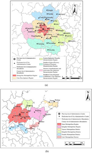
The study area includes two urban agglomerations in the middle and lower reaches of the Yellow River in China: the Central Plains Urban Agglomeration (inland urban agglomeration) and the Shandong Peninsula Urban Agglomeration (coastal urban agglomeration). According to the Central Plains Urban Agglomeration Development Plan approved by the State Council on December 28, 2016, the Central Plains Urban Agglomeration is located between 31.38° N and 37.82° N and between 110.21° E and 118.19° E and includes the whole province of Henan and some cities in Shanxi, Hebei, Shandong and Anhui provinces, covering an area of 287,000 square kilometres (as shown in Figure 1(a)). According to the Development Plan of Shandong Peninsula Urban Agglomeration (2016-2030) published by the Shandong Provincial Government in 2017, Shandong Peninsula Urban Agglomeration includes 17 cities in Shandong Province and has an overall layout of ‘two circles and four districts’ (as shown in Figure 1(b)). This agglomeration is located in the eastern coastal region and thus has obvious regional advantages in building a new pattern of internal and external openings.

Figure 1. The study area: (a) Central Plains Urban Agglomeration and (b) Shandong Peninsula Urban Agglomeration.

3.2. NTL datasets

Commonly used NTL datasets include DMSP-OLS stable NTL data, NPP-VIIRS NTL data, and LuoJia-1 data. DMSP-OLS, which acquires NTL images at a 2.7-km resolution without on-board radiometric calibration, is the most commonly used sensor for NTL research, with composites released annually between 1992 and 2013. These data have disadvantages, including the lack of on-orbit radiance calibration, saturation issues, and blooming issues (Cao et al. 2014; Cao et al. 2019; Levin et al. 2020), that limit their potential applications. NPP-VIIRS NTL data are of higher quality (e.g. have a higher spatial resolution of ∼500 m) and have a superior detection ability, but the short available time span causes problems when long-term analysis is required (Chen et al. 2021). Luojia-1 NTL data have a spatial resolution of 130 m at the nadir point and provide abundant spatial detail information (Li et al. 2019). However, these data have a shorter available time span.

Chen et al. built an extended time series (2000–2018) of NPP-VIIRS-like NTL data through a new cross-sensor calibration from DMSP-OLS NTL data (2000–2012) and a composition of monthly NPP-VIIRS NTL data (2013–2018) (Chen et al. 2021). The extended NPP-VIIRS-like NTL data (2000–2018) have an excellent spatial pattern and temporal consistency. In addition, the resulting product could be easily updated and provide a useful proxy to monitor the dynamics of demographic and socioeconomic activities for longer time periods than those of existing products. The product has been updated until 2020. This study chose the extended NPP-VIIRS-like NTL data (2000-2020) as the research NTL dataset.

3.3. Other data

To obtain the reference data of the built-up areas, the statistical data of the built-up areas for each county were derived from the China Urban Construction Statistical Yearbook and China County Seat Construction Statistical Yearbook. In this study, we used 1:1 million vector data of administrative divisions from the national Geographic Information Resources Directory Service system. To facilitate a comparison between the methods, Landsat 8 OLI imagery on the Central Plains Urban Agglomeration in 2020 was downloaded.

4. Methodology

4.1. Overall process of the proposed method

The overall process of the proposed method is illustrated in Figure 2. As shown in Figure 2, the proposed method involves three steps:

Figure 2. Overall process of the proposed method.

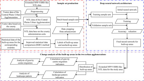
1. Sample set production: The extended NPP-VIIRS-like NTL data of the Central Plains Urban Agglomeration from 2015 to 2018 are selected for sample set production. First, the extended NPP-VIIRS-like NTL data are preprocessed by reprojection and transformation; then, the NTL data of the Central Plains Urban Agglomeration and the NTL data base on the county administration units are acquired by using the vector data of the Central Plains Urban Agglomeration and the vector data based on the county administration units respectively; using the ISDC method (shown in Section 4.2), the NTL data base on the county administration units are classified into built-up areas and nonbuilt-up areas according to the statistical data of the built-up areas; based on the classification image, the patch-based sample sets are acquired with the operation of cropping, enhancement and equalization.

2. Deep neural network architecture: Based on U-Net network, the initial neural network is constructed; then, the network is trained and adjusted by using the training sample sets and validation sample sets; the final neural network for built-up areas is completed through multiple iterations of the above operations.

3. Change analysis of the built-up areas in the two urban agglomerations: The extended NPP-VIIRS-like NTL data for the study area are input into the neural network, and the built-up areas of the two urban agglomerations are automatically extracted; then, the change analysis of the two urban agglomerations’ built-up areas is completed from the perspectives of gravity centre migration and landscape pattern.

4.2. Sample set production

The extended NPP-VIIRS-like NTL data of the Central Plains Urban Agglomeration from 2015 to 2018 were selected for sample set production. Tang (2017) showed that the logarithmic transformation of NPP-VIIRS NTL data can effectively suppress the drastic fluctuations of pixel values in the built-up area centre and enhance the homogeneity of the overall pixel value distribution. Therefore, formula (1) was used to transform the extended NPP-VIIRS-like NTL data: (1) $${\mathrm{ }DN}^{\mathrm{‘}}=\ln \hspace{0.17em}\left(DN+1\right)$$(1) where ${DN}^{‘}$ represents the pixel’s grey value after transformation and $DN$ represents the pixel’s grey value before transformation.

On the basis of He et al. (2006a), the improved statistical data comparison (ISDC) method was used to determine the built-up area and nonbuilt-up area labels of each county. The major steps of the method were as follows:

• Step 1. According to the statistical data of the built-up areas, the number of pixels belonging to the built-up areas in the extended NPP-VIIRS-like NTL data was determined and marked as N.

• Step 2. The pixel grey values of the extended NPP-VIIRS-like NTL data were rearranged into one-dimensional array A from large to small.

• Step 3. The grey value corresponding to the N^th element in array A was taken as threshold B.

• Step 4. The pixel grey values of the extended NPP-VIIRS-like NTL data were compared with threshold B, and then the labels of built-up areas and nonbuilt-up areas were determined.

The image patch size was set to 128 × 128. Since the number of pixels in the built-up area was less than that in the nonbuilt-up area, it is ensured that the central pixels of the image patch belonged to the built-up area, thereby improving the imbalance of the sample set. Considering the small volumes of the sample set, the sample set was processed for data enhancement. A total of 3200 image patches were acquired and divided into training samples and validation samples according to an 8:2 ratio.

4.3. Deep neural network architecture

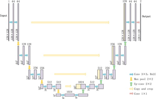
Compared to traditional optical remote sensing images, the semantic meaning of NTL data is relatively simple, and the semantic information is relatively singular. These features are similar to those of medical images, and the extraction of built-up areas is also a two-classification, semantic image segmentation task. Therefore, U-Net (Ronneberger et al. 2015), which is excellent in the field of medical image segmentation, was selected as the deep neural network architecture for the extraction of built-up areas (as shown in Figure 3). U-Net is a symmetric encoding-decoding network with a U-shaped structure. The contracting path (the left half) is an encoding structure that is composed of four downsampling modules, each of which contains two 3 × 3 convolution layers and a 2 × 2 max pooling layer. The expansive path (the right half) is a decoding structure that is composed of four upsampling modules and one output layer. Each upsampling module contains an upsampling of the feature map followed by a 2 × 2 convolution that halves the number of feature channels, a concatenation with the correspondingly cropped feature map from the contracting path, and two 3 × 3 convolution layers. At the output layer, a 1 × 1 convolution is used to map each 64-component feature vector to the desired number of classes.

Figure 3. The deep neural network architecture applied in this study.

4.4. Indicators for the change analysis of the built-up areas in the two urban agglomerations

1. Gravity centre migration indicators

   The gravity centre of the built-up areas in the urban agglomeration was calculated as the average value of the gravity centres of all built-up areas within the urban agglomeration. By calculating the gravity centre for different periods, the spatial distribution changes of the built-up areas in the urban agglomeration could be reflected. The gravity centre coordinates were calculated using formula (2): (2) $$\begin{array}{c} X_t=\frac{\sum _{i=1}^n{w}_i{x}_i}{\sum _{i=1}^n{w}_i},Y_t=\frac{\sum _{i=1}^n{w}_i{y}_i}{\sum _{i=1}^n{w}_i} \end{array}$$(2) where $X_t$ and $Y_t$ are the gravity centre coordinates of the built-up areas in the urban agglomeration in year t; $x_i$ and $y_i$ are the gravity centre coordinates of the i-th built-up area patch in the urban agglomeration; n indicates the total number of built-up area patches in the urban agglomeration; and $w_i$ indicates the weight, i.e., the area of the i-th built-up area patch divided by the total area of all built-up area patches.

   The gravity centre migration distance and direction can reflect the movement trajectory of the gravity centre and were obtained in this study as shown in formulas (3) and (4), respectively: (3) $$\begin{array}{c}{D}_{t,t+k}=\sqrt{{\left(X_{t+k}-X_t\right)}^2+{\left(Y_{t+k}-Y_t\right)}^2} \end{array}$$(3) (4) $$\begin{array}{c}{\theta }_{t,t+k}=\{\begin{array}{c}\arctan (\frac{Y_{t+k}-Y_t}{X_{t+k}-X_t}), X_{t+k}-X_t>0 \\ \arctan (\frac{Y_{t+k}-Y_t}{X_{t+k}-X_t})+\pi , X_{t+k}-X_t<0,Y_{t+k}-Y_t\ge 0\\ \arctan (\frac{Y_{t+k}-Y_t}{X_{t+k}-X_t})-\pi , X_{t+k}-X_t<0,{\mathrm{Y}}_{t+k}-Y_t<0\\ \frac{\pi }{2}, X_{t+k}-X_t=0,Y_{t+k}-Y_t>0\\ -\frac{\pi }{2}, X_{t+k}-X_t=0,Y_{t+k}-Y_t<0\\ no \mathit{migration}, X_{t+k}-X_t=0,Y_{t+k}-Y_t=0\end{array}\end{array}$$(4)

   where $D_{t,t+k}$ is the migration distance of the gravity centre of the built-up areas in the urban agglomeration from year t to year t + k; ${\theta }_{t,t+k}$ is the migration direction of the gravity centre of the built-up areas in the urban agglomeration from year t to year t + k; and $X_{t+k}$ and $Y_{t+k}$ are the gravity centre coordinates of the built-up areas in the urban agglomeration in year t + k.

2. Landscape pattern indicators

   Landscape pattern indicators can be used to express the characteristics and spatial distribution of the built-up area patches in the urban agglomeration, as shown in Table 1.

Table 1. Descriptions of landscape pattern indicators.

Type	Calculation formula	Value range	Unit	Description
Total patch area	$\mathit{TPA}={\sum }_{i=1}^n{a}_i$	TPA > 0	km^2	The total area of built-up patches
Number of patches	$NP=n$	NP > 0		The number of patches can reflect the fragmentation of the built-up patches and has a good positive correlation with the fragmentation degree of the built-up patches.
Average patch area	$\mathit{APA}=\frac{{\sum }_{i=1}^n{a}_i}{n}$	$\mathit{APA}$>0	km^2	The average patch area can reflect the average size of built-up patches.
Patch density	$PD=\frac{n}{A}\times {10}^8$	PD > 0	per 100 km^2	The patch density refers to the number of patches per 100 km2 and can reflect the density of built-up patches.
Largest patch index	$\mathit{LPI}=\frac{\mathrm{Max}(a_1,a_2,\dots ,a_n)}{A}\times 100$	0 < LPI $\le$100	%	The largest patch index is the percentage of the largest built-up patch area in the total area of the study area, indicating the impact of the largest built-up patch on the study area.
Total edge length	$\mathit{TEL}={\sum }_{i=1}^n{e}_i$	TEL > 0	km	The total edge length of all built-up patches in the study area
Average edge density	$\mathit{AED}=\frac{{\sum }_{i=1}^n{e}_i}{A}\times {10}^8$	AED $\ge$0	km per 100 km^2	The average edge density can reflect the degree of dividing the study area by the built-up patches’ boundary.
Landscape shape index	$\mathit{LSI}=\frac{0.25{\sum }_{i=1}^n{e}_i}{\sqrt{A}}$	LSI ≥ 1		The landscape shape index can reflect the shape change of the built-up patches. The larger the value is, the more complex the patch shape is.
Aggregation index	$AI=\left[\frac{g_{ii}}{\max \to g_{ii}}\right]\times 100$	0 ≤ AI ≤ 100	%	The aggregation index can reflect the connectivity between the built-up patches. The smaller the value is, the more discrete the patches are.

Notes: n represents the total numbers of the built-up patches, $a_i$ represents the area of the i-th built-up patch (${\mathrm{m}}^2),$ A represents the total area of the study area (${\mathrm{m}}^2),$ $\mathrm{Max}(a_1,a_2,\dots ,a_n)$ represents the area of the largest built-up patch in the study area (${\mathrm{m}}^2),$ $e_i$ represents the edge length of the i-th built-up patch ($km$), $g_{ii}$ represents the connectivity number between the built-up patches, and $\max \to g_{ii}$ represents the maximum connectivity number between the built-up patches.

5. Results and discussion

5.1. Evaluation of the deep neural network

Through repeated experiments, we set the batch size to 8 and the learning rate to 1e-4 for deep neural network training. The trained network was evaluated with the validation data. Precision, recall, F1 score and intersection over union (IoU) were used as the evaluation indicators, as shown in formulas (5), (6), (7) and (8), respectively. The definitions of the parameters in the formulas are shown in Table 2. TP (True Positive) refers to the number of pixels for which the real categorization is a built-up area and the category prediction by the deep neural network was also the built-up area. FP (False Positive) refers to the number of pixels for which the real category is a nonbuilt-up area and the category predicted by the deep neural network was a built-up area. FN (False Negative) refers to the number of pixels for which the real category was the built-up area and the category predicted by the deep neural network was a nonbuilt-up area. TN (True Negative) refers to the number of pixels for which the real category was the nonbuilt-up area and the category predicted by the deep neural network was also a nonbuilt-up area. (5) $$\begin{array}{c} \mathit{Precision}=\frac{TP}{TP+FP} \end{array}$$(5) (6) $$\mathit{Recall}=\frac{TP}{TP+FN}\mathrm{ }$$(6) (7) $$F1=\frac{\mathit{Precision}\times \mathit{Recall}}{\mathit{Precision}+\mathit{Recall}}\times 2$$(7) (8) $$\begin{array}{c}IoU=\frac{TP}{TP+FN+FP} \end{array}$$(8)

Table 2. The confusion matrix.

	Built-up area (ground truth)	Nonbuilt-up area (ground truth)
Built-up area (prediction)	TP	FP
Nonbuilt-up area (Prediction)	FN	TN

The precision, recall, F1 score and IoU of the trained network were found to be 0.9692, 0.9777, 0.9734 and 0.9483, respectively, on the validation data; these values all meet the accuracy requirements.

5.2. Comparison analysis

In order to prove the advantages of our method, the built-up area extraction method (BAEM) (Bhatti and Tripathi 2014), which has been cited 146 times according to the statistics of Web of Science until now, was selected as a comparison method. The BAEM method using Landsat-8 OLI imagery comprised four major steps: preprocessing and examination of satellite data, image enhancement through resolution merging, producing the BAEM_OLI imagery, and finding the optimal threshold value to segregate built-up from non-built-up areas in the BAEM_OLI imagery. Our method and BAEM method were applied simultaneously to extract the built-up areas in the Central Plains Urban Agglomeration in 2020, and compared in terms of accuracy and operational efficiency. The reference data of the built-up areas were acquired by the ISDC method (shown in Section 4.2).

5.2.1. Accuracy

As shown in Figure 4, the extraction results of our method and BAEM method were both in good agreement with the reference data in most counties. This demonstrated that both methods had high accuracy of extracting the built-up areas.

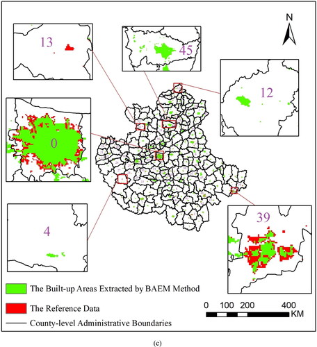
Figure 4. Extraction results of the built-up areas in the Central Plains Urban Agglomeration in 2020: (a) the built-up areas extracted by our method overlaid with the reference data, (b) the reference data overlaid with the built-up areas extracted by our method, (c) the built-up areas extracted by BAEM method overlaid with the reference data, and (d) the reference data overlaid with the built-up areas extracted by BAEM method.

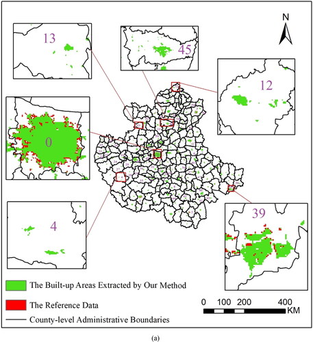
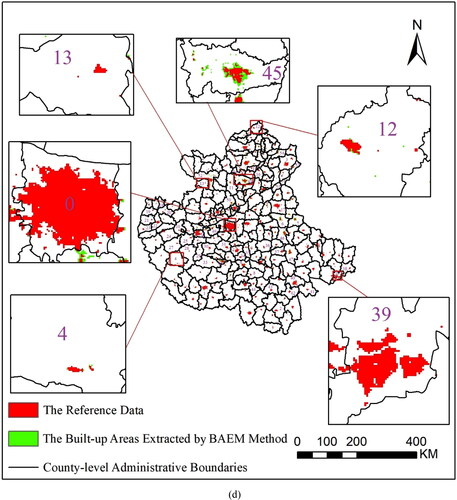
Comparing Figure 4(a) and (b), the mismatches on the ranges of the built-up areas between our method and the reference data were mainly reflected in County 0 to 12. In County 0 to 3, our method had a smaller range of built-up areas. Through field investigations, we found that in County 0 to 3, the pixels that were not identified as built-up areas by our method while belonged to built-up areas in the reference data located in the urban suburbs. Although these urban suburbs were composed of buildings, concretes, and asphalt, the social and economic activities of human beings were infrequent, and people were accustomed to calling these regions ‘ghost towns’. We preferred not to classify these regions as built-up areas. However, (Zhao et al. 2020) emphasized that the pixels that belonged to built-up areas in the urban suburbs with low intensity of human activity were easy to be ignored because of the effect of shrink of NTL. In order to further understand the reasons, the multisource data could be integrated to improve the proposed method in future research. In County 4 to 12, our method had a bigger range of built-up areas. Through field investigations, we found that in County 4 to 12, the pixels that were identified as built-up areas by our method while did not belong to built-up areas in the reference data located in the towns. With the implementation of China’s rural revitalization policy, the economic development of these towns had been rapid, and the scale of the built-up areas had been expanding. However, due to the lack of statistical data and lagging management, the built-up areas of these towns were generally not included in the statistics. This kind of built-up areas can be well recognized by our method.

Comparing Figure 4(c) and (d), the mismatches on the ranges of the built-up areas between BAEM method and the reference data were reflected in County 0 to 2, County 5 to 7, County 9, and County 13 to 54. In County 0 to 2 and County 13 to 44, BAEM method had a smaller range of built-up areas. The built-up areas of County 13 had not even been extracted at all. Through field investigations and the results from the methods of NDII (Wang et al. 2015) and CBI (Sun et al. 2016), we verified that the omission built-up areas by BAEM method in the above counties should be identified as built-up areas really. In County 5 to 7, County 9, and County 45 to 54, BAEM method had a bigger range of built-up areas. Through field investigations, we found that in these counties, the pixels that were identified as built-up areas by BAEM method while did not belong to built-up areas in the reference data mainly located in the urban suburbs. As mentioned in the previous paragraph, these urban suburbs are known as ‘ghost towns’ due to their infrequent human socio-economic activities. From a socio-economic perspective, it is reasonable to classify these urban suburbs as nonbuilt-up areas. Therefore, BAEM method has certain commission error in these counties.

As shown in Table 3, compared to BAEM method, the precision, recall, F1 score and IoU of our method increased by 7.19%, 0.30%, 3.68% and 5.78%, respectively. This shows that our method has a higher accuracy.

Table 3. Comparison of different methods.

Method	Precision	Recall	F1 score	IoU
Our method	0.9160	0.8642	0.8894	0.8008
BAEM method	0.8441	0.8612	0.8526	0.7430

5.2.2. Operational efficiency

The main hardware configuration of our operating computer was as follows:

• ① Central Processing Unit (CPU): Intel i7-4790 3.60 GHz

• ② Video adapter: NVIDIA GeForce GT 720

• ③ Random Access Memory (RAM): Hynix/Hyundai 8GB

We calculated the running time of our method and BAEM method for extracting the built-up areas in the Central Plains Urban Agglomeration in 2020 respectively.

1. Running time of our method

   Our method had a running time of 59 seconds, including: 24 seconds for model prediction; 35 seconds for prediction results post-processing. For the work of extracting the built-up areas in the Central Plains Urban Agglomeration covering an area of 287,000 square kilometres, a 59-second running time is pretty short.

2. Running time of BAEM method

   BAEM method had a cumulative running time of 8.3 hours, including: 6.4 hours for downloading, preprocessing and examination of Landsat-8 OLI imagery; 0.3 hour for image enhancement; 0.5 hour for producing the BAEM_OLI imagery; 1.1 hours for finding the optimal threshold value to segregate built-up from non-built-up areas in the BAEM_OLI imagery and producing the extraction results. Due to the influence of weather and imaging conditions, high-quality Landsat-8 OLI imageries covering the large regions were difficult to be obtained. This resulted in spending more time in the first stage. For the large region like the Central Plains Urban Agglomeration, finding the optimal threshold value is quite time-consuming. As a result, a considerable amount of time was spent in the final stage.

Comparing the running time of our method and BAEM method, we found that the operational efficiency of our method was significantly higher than that of BAEM method. Moreover, our method requires no human intervention, and the entire operation process is fully automated.

5.3. Change analysis of the built-up areas in the two urban agglomerations

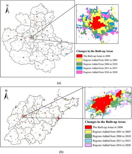
The built-up areas in the Central Plains Urban Agglomeration and Shandong Peninsula Urban Agglomeration were extracted from 2000 to 2020 based on our method. For convenience, the change results of the built-up areas were displayed in a 5-year cycle, as shown in Figure 5. The built-up areas in the two urban agglomerations grew rapidly in the past 20 years, and the growth rates of individual cities were relatively large.

Figure 5. Changes in the built-up areas in the study area from 2000 to 2020: (a) Central Plains Urban Agglomeration and (b) Shandong Peninsula Urban Agglomeration.

Tables 4 and 5 show the statistics of the gravity centre migrations of the built-up areas in the two urban agglomerations. Before 2015, the gravity centre migration distance in the Central Plains Urban Agglomeration was large, indicating that the expansion of the built-up areas in this region was unbalanced during this period, and the unidirectional expansion speed was fast. After 2015, the gravity centre migration distance in the Central Plains Urban Agglomeration was small, indicating that the expansion of built-up areas in this region was relatively balanced during this period. The gravity centre migration distance in the Shandong Peninsula Urban Agglomeration was disorderly and fluctuated greatly.

Table 4. The statistics of the gravity centre migration of the built-up areas in the Central Plains Urban Agglomeration.

Year	X coordinate (m)	Y coordinate (m)	Migration distance (km)	Migration direction (degree)	Remarks
2000	813287.41	3750585.42			The gravity centre of the built-up areas in the previous year was set as the origin of the coordinate axis, and the following coordinate system of the migration direction was established. Notes: The Y axis is the north direction, and the X axis is the east direction.
2001	809663.72	3765045.85	14.91	104.07
2002	805639.48	3748628.10	16.90	−103.77
2003	812316.54	3740823.85	10.27	−49.45
2004	809719.51	3742417.02	3.05	148.47
2005	803127.77	3738681.01	7.58	−150.46
2006	811778.70	3735797.50	9.12	−18.43
2007	821749.30	3726795.12	13.43	−42.08
2008	815813.28	3723487.25	6.80	−150.87
2009	821691.83	3737095.59	14.82	66.64
2010	826950.46	3725605.76	12.64	−65.41
2011	829890.45	3721627.84	4.95	−53.53
2012	829678.92	3727594.77	5.97	92.03
2013	829521.63	3716064.03	11.53	−90.78
2014	837365.63	3716242.52	7.85	1.30
2015	841705.35	3714279.95	4.76	−24.33
2016	842490.85	3713648.03	1.01	−38.82
2017	841667.76	3712200.30	1.67	−119.62
2018	841869.40	3711005.38	1.21	−80.42
2019	840856.85	3712657.74	1.94	121.50
2020	839869.74	3713138.12	1.10	154.05

Table 5. The statistics of the gravity centre migration of the built-up areas in the Shandong Peninsula Urban Agglomeration.

Year	X coordinate (m)	Y coordinate (m)	Migration distance (km)	Migration direction (degree)	Remarks
2000	1184962.75	3966467.83			The gravity centre of the built-up areas in the previous year was set as the origin of the coordinate axis, and the following coordinate system of the migration direction was established. Notes: The Y axis is the north direction, and the X axis is the east direction.
2001	1187833.72	3970144.15	4.66	52.01
2002	1180253.30	3964134.97	9.67	−141.60
2003	1187336.91	3966743.51	7.55	20.22
2004	1182284.83	3961566.14	7.23	−134.30
2005	1183046.87	3962406.31	1.13	47.79
2006	1189501.68	3961308.70	6.55	−9.65
2007	1192738.75	3960306.47	3.39	−17.20
2008	1193096.84	3961502.66	1.25	73.33
2009	1184525.51	3957356.73	9.52	−154.19
2010	1183208.81	3958405.37	1.68	141.47
2011	1182604.38	3957872.33	0.81	−138.59
2012	1174984.17	3955409.34	8.01	−162.09
2013	1177924.01	3956889.60	3.29	26.73
2014	1176144.51	3955113.99	2.51	−135.06
2015	1177952.45	3955068.48	1.81	−1.44
2016	1177911.58	3955161.81	0.10	113.65
2017	1174734.31	3953310.67	3.68	−149.77
2018	1176158.91	3953562.81	1.45	10.04
2019	1172289.24	3953400.81	3.87	−177.60
2020	1172814.07	3952513.07	1.03	−59.41

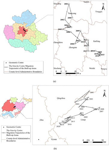
The gravity centre migration trajectories of the built-up areas in the Central Plains Urban Agglomeration and Shandong Peninsula Urban Agglomeration are shown in Figure 6. From 2000 to 2020, the gravity centre of the built-up areas in the Central Plains Urban Agglomeration was located in the metropolitan area of Zhengzhou, close to the geometric centre of the agglomeration. In 2000, the gravity centre was located in Yuanyang County, Xinxiang City. In 2003, it moved to Zhongmou County, Zhengzhou City. In 2010, it moved to the Kaifeng municipal district. In terms of the migration directions, it migrated 8 times south-eastward, 5 times south-westward, 2 times north-eastward, and 5 times north-westward. Compared to the gravity centre in 2000, it ultimately migrated south-eastward. It can be judged that the northern cities with relatively high development degrees had slower expansion speeds, while the southern cities with lower development degrees had faster expansion speeds. The cities in the eastern region expanded faster than those in the western region. From 2000 to 2020, the gravity centre of the built-up areas in the Shandong Peninsula Urban Agglomeration was located in the Qingdao metropolitan area. Excluding 2001 (located in Qingzhou City) and 2002 (located at the junction of Qingzhou City and Linqu County), the gravity centre was located in Weifang City Linqu County. In terms of the migration directions, it migrated 4 times south-eastward, 8 times south-westward, 6 times north-eastward, and 2 times north-westward. From 2000 to 2007, the gravity centre shifted south-eastward, and from 2008 to 2020, it shifted south-westward. Compared to the gravity centre in 2000, it finally migrated south-westward. It can be judged that the northern cities with relatively high development degrees had slower expansion speeds, while the southern cities with lower development degrees had faster expansion speeds. Before 2007, the eastern cities expanded faster than the western cities, and after 2007, the western cities expanded faster than the eastern cities.

Figure 6. The gravity centre migration trajectories of the built-up areas in the study area from 2000 to 2020: (a) Central Plains Urban Agglomeration and (b) Shandong Peninsula Urban Agglomeration.

Table 6 shows the calculation results of the landscape pattern indicators of the built-up areas in the Central Plains Urban Agglomeration. The TPA increased rapidly from 2000 to 2020, with an average annual growth rate of 8.53% and a total increase of 4.14 times. This shows that the scope of the built-up area expanded rapidly over the past 21 years. The change trends of NP and PD were the same and increased at average annual growth rates of 7.14% and 7.42%, respectively. The NP and PD increased significantly in 2012 and 2013, which indicates that a large number of emerging towns appeared during this period, and the agglomeration entered the stage of high-speed development. After 2013, these two indicators fell back, which indicates that emerging cities and towns began to integrate and connect with large urban patches.

Table 6. The calculation results of the landscape pattern indicators of the built-up areas in the Central Plains Urban Agglomeration.

Year	TPA (km^2)	NP	PD (per 100 km^2)	LPI (%)	TEL (km)	AED (km per 100 km^2)	LSI	AI (%)
2000	1665.50	328	0.11	0.0314	3236.0	1.132	19.7378	76.6489
2001	1847.50	336	0.12	0.0490	3373.0	1.180	19.6163	78.0805
2002	2599.00	414	0.14	0.0680	4576.0	1.601	22.4657	78.7303
2003	2712.00	396	0.14	0.0781	4679.0	1.637	22.3971	79.1874
2004	3558.00	464	0.16	0.0767	6154.0	2.153	25.7741	79.0221
2005	3508.00	442	0.15	0.0838	5852.0	2.047	24.7089	79.8074
2006	3638.75	433	0.15	0.0984	5743.5	2.009	23.7479	80.9304
2007	3577.75	474	0.17	0.0868	6005.0	2.101	25.0333	79.6773
2008	3787.75	471	0.16	0.1125	6174.0	2.160	24.9960	80.2795
2009	3736.00	509	0.18	0.0836	6451.0	2.257	26.3306	79.0642
2010	4203.50	617	0.22	0.1014	7639.5	2.672	29.3923	77.8770
2011	4976.50	654	0.23	0.1438	7997.0	2.798	28.2933	80.4599
2012	4944.50	905	0.32	0.0937	8890.5	3.110	31.5496	78.0644
2013	6387.25	1240	0.43	0.1374	11448.0	4.005	35.8563	78.0338
2014	6730.00	1125	0.39	0.1439	11164.5	3.906	34.0213	79.6976
2015	6771.75	1092	0.38	0.1445	11146.5	3.899	33.8424	79.8715
2016	6827.00	1095	0.38	0.1474	11417.0	3.994	34.5559	79.5395
2017	7403.25	1137	0.40	0.1795	11955.5	4.182	34.7217	80.2415
2018	7771.00	1166	0.41	0.1957	12519.5	4.380	35.5411	80.2750
2019	8198.00	1211	0.42	0.1867	13049.5	4.565	36.0165	80.5109
2020	8568.25	1303	0.46	0.2043	13836.0	4.840	37.3450	80.2215
Annual growth rate	8.53%	7.14%	7.42%	9.82%	7.54%	7.54%	3.24%	8.53%

The average annual growth rate of the LPI was 9.82%, which was higher than that of the TPA. This shows that the Zhengzhou metropolitan area expands faster than all built-up areas in the Central Plains Urban Agglomeration. Moreover, the LPI showed an increasing trend year by year, which indicates that the influence of the Zhengzhou metropolitan area in the Central Plains Urban Agglomeration is constantly increasing. As the development core of the networked spatial pattern in the Central Plains Urban Agglomeration, the Zhengzhou metropolitan area has played a good radiation role, fulfilled the responsibility of ‘one core’, achieved deep integration with surrounding cities, and further promoted the development of peripheral cities.

The change trends of the TEL, AED and LSI increased each year, with average annual growth rates of 7.54%, 7.54% and 3.24%, respectively. This shows that the shape complexity of the built-up areas in the Central Plains Urban Agglomeration was gradually increasing, and the scope of the built-up areas was gradually expanding. Taking 2014 as the dividing point, the average growth rate of the LSI from 2000 to 2013 was 4.70%, and the average growth rate from 2014 to 2020 was 1.57%. These results indicate that with the passage of time, the increase rate of the shape complexity of the built-up areas in the Central Plains Urban Agglomeration decelerated, and the overall expansion speed in the latter stage was slower than that in the previous stage. Before 2014, the data fluctuated greatly, showing that the expansion of the built-up areas in this stage was not stable from the perspective of spatial characteristics.

The AI generally rose from 2000 to 2020. This shows that the fragmentation degree of the built-up areas in the urban agglomeration tended to be low, and the links between cities and towns became increasingly close throughout the study period. However, the AI fluctuated violently and showed a trend of rising, falling and rising. From 2001 to 2014, the fluctuations were extremely sharp, indicating that the urban expansion in this stage was unstable. From 2015 to 2020, the fluctuations decelerated, indicating that the urban expansion in this stage tended to be stable, and the Central Plains Urban Agglomeration gradually transitioned from high-speed development to high-quality development.

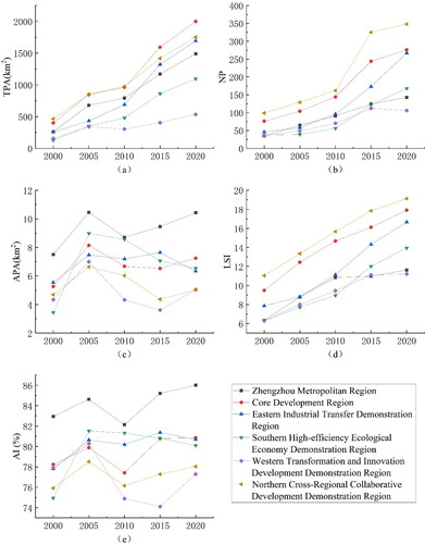
According to the development plan of the Central Plains Urban Agglomeration, the agglomeration can be divided into six main regions: the Zhengzhou Metropolitan Region, Core Development Region, Eastern Industrial Transfer Demonstration Region, Southern High-efficiency Ecological Economy Demonstration Region, Western Transformation and Innovation Development Demonstration Region and Northern Cross-Regional Collaborative Development Demonstration Region (Figure 1(a)). Considering a five-years cycle, five landscape pattern indicators, including the TPA, NP, APA, LSI and AI, were adopted to analyse the status of the built-up areas in these six main regions (Figure 7). Figure 7 shows that the status of the built-up areas in various regions exhibited obvious differences. The APA and AI of the Zhengzhou Metropolitan Region had the highest values, reflecting the highest development degree of the region. The five indicators of the Western Transformation and Innovation Development Demonstration Region were not high, and this region was relatively underdeveloped overall. Figure 7(a) (b) and (d) shows that the TPA, NP and LSI of the Core Development Region and Northern Cross-Regional Collaborative Development Demonstration Region were relatively high. This reflects the large-scale and rapid development of the built-up areas in these two regions, providing is an important basis for supporting the development of the Central Plains Urban Agglomeration. Although the development speed and scale of the Eastern Industrial Transfer Demonstration Region and Southern High-efficiency Ecological Economy Demonstration Region were not as fast as those of the Core Development Region and Northern Cross-Regional Collaborative Development Demonstration Region, the APA and AI of these two regions have performed well in recent years, reflecting the obvious trend of the integration of the built-up areas in these two regions.

Figure 7. The changes in the typical landscape pattern indicators in the six main regions of the Central Plains Urban Agglomeration: (a) TPA, (b) NP, (c) APA, (d) LSI, and (e) AI.

Table 7 shows the calculation results of the landscape pattern indicators of the built-up areas in the Shandong Peninsula Urban Agglomeration. The TPA increased rapidly from 2000 to 2020, with an average annual growth rate of 6.8% and a total increase of 3.73 times. The change trends of the NP and PD were the same and increased at average annual growth rates of 8.82% and 8.86%, respectively. The Shandong Peninsula Urban Agglomeration is a dual-core urban agglomeration containing Jinan and Qingdao. The built-up areas of these two cities alternately became the largest patches, causing the LPI of the urban agglomeration to fluctuate, but the overall trend was upwards, with an average annual growth rate of 5.7%.

Table 7. The calculation results of the landscape pattern indicators of the built-up areas in the Shandong Peninsula Urban Agglomeration.

Year	TPA (km^2)	NP	PD (per 100 km^2)	LPI (%)	TEL (km)	AED (km per 100 km^2)	LSI	AI (%)
2000	1828.00	205	0.13	0.0906	2911.0	1.868	17.1860	80.7362
2001	2149.75	250	0.16	0.1126	3442.0	2.208	18.7634	80.5784
2002	2463.00	314	0.20	0.1030	4133.0	2.652	21.0804	79.5129
2003	2844.50	338	0.22	0.1163	4645.0	2.980	22.0280	80.0373
2004	3348.75	386	0.25	0.1156	5651.5	3.626	24.7328	79.2680
2005	3467.50	367	0.24	0.1193	5584.5	3.583	23.9873	80.2756
2006	3597.75	385	0.25	0.1678	5775.0	3.705	24.3958	80.3272
2007	3735.50	334	0.21	0.1647	5425.5	3.481	22.4286	82.2869
2008	3866.50	432	0.28	0.1517	6269.5	4.022	25.5783	80.0541
2009	3901.00	351	0.23	0.1862	5711.5	3.664	23.1560	82.1080
2010	4166.00	580	0.37	0.1468	7703.5	4.942	30.1506	77.1689
2011	4203.75	620	0.40	0.1752	7463.5	4.788	29.0538	78.1420
2012	4316.50	572	0.37	0.1296	7401.5	4.749	28.5437	78.8614
2013	5127.75	957	0.61	0.1660	9603.5	6.161	33.9617	76.7767
2014	5510.75	911	0.58	0.1803	9753.0	6.257	33.3165	78.0813
2015	5530.25	947	0.61	0.1788	9928.5	6.370	33.8154	77.7467
2016	5632.25	940	0.60	0.1894	9856.0	6.323	33.2326	78.3229
2017	6052.25	950	0.61	0.2254	10243.0	6.572	33.3141	79.0421
2018	6288.75	1033	0.66	0.2177	10818.0	6.941	34.4937	78.6946
2019	6441.00	1035	0.66	0.2523	11066.0	7.100	34.7733	78.7623
2020	6814.00	1112	0.71	0.2743	11724.5	7.522	35.8248	78.7250
Annual growth rate	6.8%	8.82%	8.86%	5.7%	7.21%	7.21%	3.74%	−0.13%

The change trends of the TEL, AED and LSI increased each year, with average annual growth rates of 7.21%, 7.21% and 3.74%, respectively. These results show that the shape complexity of the built-up areas in the Shandong Peninsula Urban Agglomeration was gradually increasing, and the scope of the built-up areas was gradually expanding. The average growth rate of the LSI was 5.37% before 2013 and 0.89% after 2013. This shows that the growth rate of the shape complexity of the built-up areas in the Shandong Peninsula Urban Agglomeration decelerated over time. Moreover, before 2013, the TEL, AED and LSI values fluctuated greatly, indicating that the urban expansion at this stage was not stable from the perspective of spatial characteristics and that the scope of the built-up areas was in a period of rapid expansion.

The AI fluctuated sharply and showed a trend of rising first, then falling and then rising again. However, from 2000 to 2020, the overall trend was downwards. This shows that the fragmentation degree of the built-up areas in the Shandong Peninsula Urban Agglomeration was rising, and the spatial pattern of the built-up areas was more scattered than the original. The fluctuations between 2001 and 2014 were extremely sharp, and this further explained the instability of urban expansion at this stage. From 2015 to 2020, the fluctuations decelerated and an overall upwards trend was observed, indicating that urban expansion was gradually stable and tended towards agglomeration during this stage.

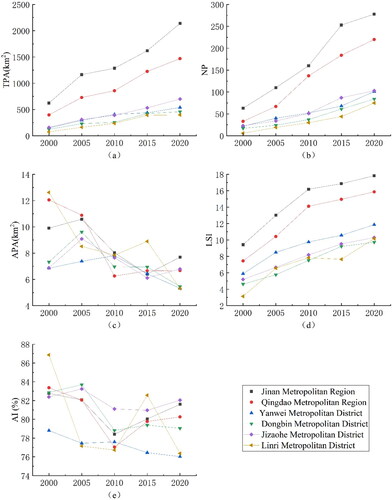
In the Development Plan of Shandong Peninsula Urban Agglomeration (2016-2030), the Shandong Peninsula Urban Agglomeration is divided into six major areas, namely, the Jinan Metropolitan Region, Qingdao Metropolitan Region, Yanwei Metropolitan District, Dongbin Metropolitan District, Jizaohe Metropolitan District and Linri Metropolitan District, and the overall pattern of ‘two regions and four districts, network development’ could be constructed. Figure 8 shows the changes in the TPA, NP, APA, LSI and AI values in these six areas from 2000 to 2020. From Figure 8(a) (b) and (d), it can be seen that the six areas were in a rapid development trend since 2000, and among them, the Jinan Metropolitan Region and Qingdao Metropolitan Region developed fastest. As shown in Figure 8(c) and (e), the APA and AI of the six areas fluctuated greatly and showed downwards trends. These results indicate that the six areas were still in a decentralized development state and that the integration and interconnection of the urban built-up areas was not sufficient.

Figure 8. The changes in the landscape pattern indicators of the six areas in the Shandong Peninsula Urban Agglomeration from 2000 to 2020: (a) TPA, (b) NP, (c) APA, (d) LSI, and (e) AI.

6. Conclusions

This study proposed a deep learning method to extract the built-up areas using NTL data, and applied the method to analyze the spatial and temporal changes of the built-up areas in Chinese two urban agglomerations from 2000 to 2020. The built-up areas for extracting by the proposed method were in good agreement with the reference data. Compared with BAEM method, our method had a higher accuracy and higher operational efficiency.

During the past few decades, the gravity centre of the built-up areas in the Central Plains Urban Agglomeration migrated south-eastward, and the gravity centre of the built-up areas in the Shandong Peninsula Urban Agglomeration migrated south-westward, with these gravity centres gradually approaching the geometric centres of the corresponding urban agglomerations. The built-up areas in the Central Plains and Shandong Peninsula Urban Agglomerations grew rapidly, increasing by 4.14 times and 3.73 times from 2000 to 2020, respectively. The built-up areas in the Central Plains Urban Agglomeration expanded faster, while the urban development degree of the Shandong Peninsula Urban Agglomeration was higher. The urban distributions and development modes of these two urban agglomerations were quite different. The Central Plains Urban Agglomeration tended to further agglomerate, while the Shandong Peninsula Urban Agglomeration tended to disperse.

This study opens new research avenues for the long-term and reliable monitoring of built-up areas in large regions using NTL data. The proposed method shows great potentials in extracting the built-up areas. In future research, multisource data, such as Landsat OLI, land surface temperature (LST), normalized difference vegetation index (NDVI), and point-of-interest (POI) data, could be integrated to improve the accuracy of the proposed method. In terms of NTL data, other NTL data could also be used, such as LuoJia1-01 Jilin-1 data.

Disclosure statement

No potential conflict of interest was reported by the authors.

Additional information

Funding

Henan Provincial Science and Technology Research Project; National Natural Science Foundation of China;

References

- Bhatti SS, Tripathi NK. 2014. Built-up area extraction using Landsat 8 OLI imagery. GIScience Remote Sens. 51(4):445–467. doi: 10.1080/15481603.2014.939539.
- Cao X, Chen J, Imura H, Higashi O. 2009. A SVM-based method to extract urban areas from DMSP-OLS and SPOT VGT data. Remote Sens Environ. 113(10):2205–2209. doi: 10.1016/j.rse.2009.06.001.
- Cao X, Hu Y, Zhu X, Shi F, Zhuo L, Chen J. 2019. A simple self-adjusting model for correcting the blooming effects in DMSP-OLS nighttime light images. Remote Sens Environ. 224:401–411. doi: 10.1016/j.rse.2019.02.019.
- Cao X, Wang J, Chen J, Shi F. 2014. Spatialization of electricity consumption of China using saturation-corrected DMSP-OLS data. Int J Appl Earth Obs Geoinf. (28), :193–200. doi: 10.1016/j.jag.2013.12.004.
- Carlson TN, Arthur ST. 2000. The impact of land use – land cover changes due to urbanization on surface microclimate and hydrology: a satellite perspective. Global Planet Change. 25(1-2):49–65. doi: 10.1016/S0921-8181(00)00021-7.
- Cengiz S, Görmüş S, Oğuz D. 2022. Analysis of the urban growth pattern through spatial metrics; Ankara City. Land Use Policy. 112:105812. doi: 10.1016/j.landusepol.2021.105812.
- Chang R, Hou D, Chen Z, Chen L. 2023. Automatic extraction of urban impervious surface based on Sah-Unet. Remote Sens. 15(4):1042. doi: 10.3390/rs15041042.
- Chen Z, Yu B, Yang C, Zhou Y, Yao S, Qian X, Wang C, Wu B, Wu J. 2021. An extended time series (2000–2018) of global NPP-VIIRS-like nighttime light data from a cross-sensor calibration. Earth Syst Sci Data. 13(3):889–906. doi: 10.5194/essd-13-889-2021.
- Chettry V. 2022. Geospatial measurement of urban sprawl using multi‑temporal datasets from 1991 to 2021: case studies of four Indian medium‑sized cities. Environ Monit Assess. 194(12):860. doi: 10.1007/s10661-022-10542-6.
- Deng C, Wu C. 2012. Bci: a biophysical composition index for remote sensing of urban environments. Remote Sens Environ. 127(12):247–259. doi: 10.1016/j.rse.2012.09.009.
- Elvidge CD, Baugh KE, Kihn EA, Kroehl HW, Davis ER. 1997a. Mapping city lights with nighttime data from the DMSP operational linescan system. Photogramm Eng Remote Sens. 63(6):727–734.
- Elvidge CD, Baugh KE, Kihn EA, Kroehl HW, Davis ER, Davis CW. 1997b. Relation between satellite observed visible-near infrared emissions, population, economic activity and electric power consumption. Int J Remote Sens. 18(6):1373–1379. doi: 10.1080/014311697218485.
- Elvidge CD, Baugh K, Zhizhin M, Hsu F. 2013a. Why VIIRS data are superior to DMSP for mapping nighttime lights. APAN Proc. 35(0):62–69. doi: 10.7125/APAN.35.7.
- Elvidge CD, Imhoff ML, Baugh KE, Hobson VR, Nelson I, Safran J, Dietz JB, Tuttle BT., 2001. Night-time lights of the world: 1994-1995. ISPRS J Photogramm Remote Sens. 56(2):81–99. doi: 10.1016/S0924-2716(01)00040-5.
- Elvidge CD, Zhizhin M, Hsu FC, Baugh K. 2013b. What is so great about nighttime VIIRS data for the detection and characterization of combustion sources. APAN Proc. 35(0):33–48. doi: 10.7125/APAN.35.5.
- Elvidge CD, Zhizhin M, Hsu FC, Baugh KE. 2013c. VIIRS nightfire: satellite pyrometry at night. Remote Sens. 5(9):4423–4449. doi: 10.3390/rs5094423.
- Fang C. 2015. Important progress and future direction of studies on China’s urban agglomerations. J Geogr Sci. 25(8):1003–1024. doi: 10.1007/s11442-015-1216-5.
- Fang C, Yu D. 2017. Urban agglomeration: an evolving concept of an emerging phenomenon. Landscape Urban Plann. 162:126–136. doi: 10.1016/j.landurbplan.2017.02.014.
- Feng Y, Wang X, Du W, Liu J, Li Y. 2019. Spatiotemporal characteristics and driving forces of urban sprawl in China during 2003-2017. J Cleaner Prod. 241:118061. doi: 10.1016/j.jclepro.2019.118061.
- He C, Liu Z, Gou S, Zhang Q, Zhang J, Xu L. 2019. Detecting global urban expansion over the last three decades using a fully convolutional network. Environ Res Lett. 14(3):034008. doi: 10.1088/1748-9326/aaf936.
- Henderson M, Yeh ET, Gong P, Elvidge C, Baugh K. 2003. Validation of urban boundaries derived from global night-time satellite imagery. Int J Remote Sens. 24(3):595–609. doi: 10.1080/01431160304982.
- He C, Shi P, Li J, Chen J, Pan Y, Li J, Zhuo L, Ichinose T. 2006b. Restoring urbanization process in China in the 1990s by using non-radiancecalibrated DMSP/OLS nighttime light imagery and statistical data. Chin Sci Bull. 51(13):1614–1620. doi: 10.1007/s11434-006-2006-3.
- He C, Shi P, Li J, Chen J, Pan Y, Li J, Zhuo L, Ichinose T., 2006a. Research on the spatial process reconstruction of urbanization in Chinese mainland in 1990s based on DMSP/OLS night light data and statistical data. Chin Sci Bull. 51(13):1614–1620. doi: 10.1007/s11434-006-2006-3.
- He X, Zhou C, Zhang J, Yuan X. 2020. Using wavelet transforms to fuse nighttime light data and POI big data to extract urban built-up areas. Remote Sens. 12(23):3887. doi: 10.3390/rs12233887.
- Horton KG, Nilsson C, Van Doren BM, La Sorte FA, Dokter AM, Farnsworth A. 2019. Bright lights in the big cities: migratory birds’ exposure to artificial light. Front Ecol Environ. 17(4):209–214. doi: 10.1002/fee.2029.
- Hu X, Qian Y, Pickett STA, Zhou W. 2020. Urban mapping needs up-to-date approaches to provide diverse perspectives of current urbanization: a novel attempt to map urban areas with nighttime light data. Landscape Urban Plann. 195:103709. doi: 10.1016/j.landurbplan.2019.103709.
- Huang F, Yu Y, Feng T. 2019. Automatic extraction of impervious surfaces from high resolution remote sensing images based on deep learning. J Vis Commun Image Represent. 58:453–461. doi: 10.1016/j.jvcir.2018.11.041.
- Imhoff ML, Lawrence WT, Stutzer DC, Elvidge CD. 1997. A technique for using composite DMSP/OLS “city lights” satellite data to map urban area. Remote Sens Environ. 61(3):361–370. doi: 10.1016/S0034-4257(97)00046-1.
- Jing W, Yang Y, Yue X, Zhao X. 2015. Mapping urban areas with integration of DMSP/OLS nighttime light and MODIS data using machine learning techniques. Remote Sens. 7(9):12419–12439. doi: 10.3390/rs70912419.
- Katz Y, Levin N. 2016. Quantifying urban light pollution—a comparison between field measurements and EROS-B imagery. Remote Sens Environ. 177:65–77. doi: 10.1016/j.rse.2016.02.017.
- Lecun Y, Bengio Y, Hinton GE. 2015. Deep learning. Nature. 521(7553):436–444. doi: 10.1038/nature14539.
- Levin N, Johansen K, Hacker JM, Phinn S. 2014. A new source for high spatial resolution night time images—the EROS-B commercial satellite. Remote Sens Environ. 149:1–12. doi: 10.1016/j.rse.2014.03.019.
- Levin N, Kyba CCM, Zhang Q, De Miguel AS, Roman MO, Li X, Portnov BA, Molthan AL, Jechow A, Miller SD, et al. 2020. Remote sensing of night lights: a review and an outlook for the future. Remote Sens Environ. 237:111443. doi: 10.1016/j.rse.2019.111443.
- Li C, Duan P, Wang M, Li J, Zhang B. 2021. The extraction of built-up areas in Chinese mainland cities based on the local optimal threshold method using NPP-VIIRS images. J Indian Soc Remote Sens. 49(2):233–248. doi: 10.1007/s12524-020-01209-1.
- Li X, Li X, Li D, He X, Jendryke M. 2019. A preliminary investigation of Luojia-1 night-time light imagery. Remote Sens Lett. 10(6):526–535. doi: 10.1080/2150704X.2019.1577573.
- Liu Z, He C, Zhang Q, Huang Q, Yang Y. 2012. Extracting the dynamics of urban expansion in China using DMSP-OLS nighttime light data from 1992 to 2008. Landscape Urban Plann. 106(1):62–72. doi: 10.1016/j.landurbplan.2012.02.013.
- Liu C, Huang X, Zhu Z, Chen H, Tang X, Gong J. 2019. Automatic extraction of built-up area from ZY3 multi-view satellite imagery: analysis of 45 global cities. Remote Sens Environ. 226:51–73. doi: 10.1016/j.rse.2019.03.033.
- Liu C, Shao Z, Chen M, Luo H. 2013. MNDISI: a multi-source composition index for impervious surface area estimation at the individual city scale. Remote Sens. Lett. 4(8):803–812. doi: 10.1080/2150704X.2013.798710.
- Li X, Zhao L, Li D, Xu H. 2018. Mapping urban extent using Luojia 1-01 nighttime light imagery. Sensors. 18(11):3665. doi: 10.3390/s18113665.
- Li X, Zhou Y. 2017. Urban mapping using DMSP/OLS stable night-time light: a review. Int J Remote Sens. 38(21):6030–6046. doi: 10.1080/01431161.2016.1274451.
- Ouyang Z, Lin M, Chen J, Fan P, Qian SS, Park H. 2019. Improving estimates of built-up area from night time light across globally distributed cities through hierarchical modeling. Sci Total Environ. 647:1266–1280. doi: 10.1016/j.scitotenv.2018.08.015.
- Parekh JR, Poortinga A, Bhandari B, Mayer T, Saah D, Chishtie F. 2021. Automatic detection of impervious surfaces from remotely sensed data using deep learning. Remote Sens. 13(16):3166. doi: 10.3390/rs13163166.
- Ronneberger O, Fischer P, Brox T. 2015. U-net: convolutional networks for biomedical image segmentation. In: Navab N, Hornegger J, Wells W, Frangi A, editors. Medical Image Computing and Computer-Assisted Intervention-MICCAI 2015. Lecture Notes in Computer Science, vol 9351. Cham: Springer. doi: 10.1007/978-3-319-24574-4_28.
- Sharma RC, Tateishi R, Hara K, Gharechelou S, Iizuka K. 2016. Global mapping of urban built-up areas of year 2014 by combining MODIS multispectral data with VIIRS nighttime light data. Int J Digital Earth. 9(10):1004–1020., doi: 10.1080/17538947.2016.1168879.
- Shi K, Chen Y, Li L, Huang C. 2018. Spatiotemporal variations of urban CO2 emissions in China: a multiscale perspective. Appl Energy. 211:218–229. doi: 10.1016/j.apenergy.2017.11.042.
- Shi K, Chen Y, Yu B, Xu T, Chen Z, Liu R, Li L, Wu J. 2016. Modeling spatiotemporal CO2 (carbon dioxide) emission dynamics in China from DMSP-OLS nighttime stable light data using panel data analysis. Appl Energy. 168:523–533. doi: 10.1016/j.apenergy.2015.11.055.
- Shi K, Huang C, Yu B, Yin B, Huang Y, Wu J. 2014. Evaluation of NPP-VIIRS night-time light composite data for extracting built-up urban areas. Remote Sens Lett. 5(4):358–366. doi: 10.1080/2150704X.2014.905728.
- Shi L, Ling F, Ge Y, Foody GM, Li X, Wang L, Zhang Y, Du Y. 2017. Impervious surface change mapping with an uncertainty-based spatial-temporal consistency model: a case study in Wuhan city using Landsat time-series datasets from 1987 to 2016. Remote Sens. 9(11):1148. doi: 10.3390/rs9111148.
- Shojaei H, Nadi S, Shafizadeh-Moghadam H, Tayyebi A, Van Genderen J. 2022. An efficient built-up land expansion model using a modified U-net. Int J Digital Earth. 15(1):148–163. doi: 10.1080/17538947.2021.2017035.
- Small C, Pozzi F, Elvidge CD. 2005. Spatial analysis of global urban extent from DMSP-OLS night lights. Remote Sens Environ. 96(3-4):277–291. doi: 10.1016/j.rse.2005.02.002.
- Sun G, Chen X, Jia X, Yao Y, Wang Z. 2016. Combinational build-up index (CBI) for effective impervious surface mapping in urban areas. IEEE J Sel Top Appl Earth Observ Remote Sens. 9(5):2081–2092. doi: 10.1109/JSTARS.2015.2478914.
- Sun L, Tang L, Shao G, Qiu Q, Lan T, Shao J. 2020. A machine learning-based classification system for urban built-up areas using multiple classifiers and data sources. Remote Sens. 12(1):91. doi: 10.3390/rs12010091.
- Sutton P, Roberts D, Elvidge C, Baugh K. 2001. Census from heaven: an estimate of the global human population using night-time satellite imagery. Int J Remote Sens. 22(16):3061–3076. doi: 10.1080/01431160010007015.
- Tang M. 2017. Urban built-up area extraction from logarithm transformed NPP-VIIRS nighttime light composite data. Shanghai: East China Normal University.
- Wang Z, Gang C, Li X, Chen Y, Li J. 2015. Application of a normalized difference impervious index (NDII) to extract urban impervious surface features based on Landsat TM images. Int J Remote Sens. 36(4):1055–1069. doi: 10.1080/01431161.2015.1007250.
- Wang H, Gong X, Wang B, Deng C, Cao Q. 2021. Urban development analysis using built-up area maps based on multiple high-resolution satellite data. Int J Appl Earth Obs Geoinf. 103:102500. doi: 10.1016/j.jag.2021.102500.
- Wang J, Wu Z, Wu C, Cao Z, Fan W, Tarolli P. 2017. Improving impervious surface estimation: an integrated method of classification and regression trees (CART) and linear spectral mixture analysis (LSMA) based on error analysis. GIScience Remote Sens. 55(4):583–603. doi: 10.1080/15481603.2017.1417690.
- Xie Y, Weng Q. 2016. Updating urban extents with nighttime light imagery by using an object-based thresholding method. Remote Sens Environ. 187:1–13. doi: 10.1016/j.rse.2016.10.002.
- Xu H. 2008. A new index for delineating built-up land features in satellite imagery. Int J Remote Sens. 29(14):4269–4276. doi: 10.1080/01431160802039957.
- Xu H. 2010. Analysis of impervious surface and its impact on urban heat environment using the normalized difference impervious surface index (NDISI). Photogramm Eng Remote Sens. 76(5):557–565. doi: 10.14358/PERS.76.5.557.
- Xu T, Coco G, Gao J. 2020. Extraction of urban built-up areas from nighttime lights using artificial neural network. Geocarto Int. 35(10):1049–1066. doi: 10.1080/10106049.2018.1559887.
- Yin R, He G, Wang G, Long T, Li H, Zhou D, Gong C. 2022. Automatic framework of mapping impervious surface growth with long-term Landsat imagery based on temporal deep learning model. IEEE Geosci Remote Sens Lett. 19:1–5. doi: 10.1109/LGRS.2021.3135869.
- Yuan Q, Shen H, Li T, Li Z, Li S, Jiang Y, Xu H, Tan W, Yang Q, Wang J, et al. 2020. Deep learning in environmental remote sensing: achievements and challenges. Remote Sens Environ. 241(5):111716. doi: 10.1016/j.rse.2020.111716.
- Zhang X, Du S. 2015. A linear dirichlet mixture model for decomposing scenes: application to analyzing urban functional zonings. Remote Sens Environ. 169:37–49. doi: 10.1016/j.rse.2015.07.017.
- Zhao N, Liu Y, Cao G, Samson EL, Zhang J. 2017. Forecasting China’s GDP at the pixel level using nighttime lights time series and population images. GIScience Remote Sens. 54(3):407–425. doi: 10.1080/15481603.2016.1276705.
- Zhao X, Yu B, Liu Y, Yao S, Lian T, Chen L, Yang C, Chen Z, Wu J. 2018. NPP-VIIRS DNB daily data in natural disaster assessment: evidence from selected case studies. Remote Sens. 10(10):1526. doi: 10.3390/rs10101526.
- Zhao M, Zhou Y, Li X, Cao W, He C, Yu B, Li X, Elvidge CD, Cheng W, Zhou C. 2019. Applications of satellite remote sensing of nighttime light observations: advances, challenges, and perspectives. Remote Sens. 11(17):1971. doi: 10.3390/rs11171971.
- Zhao M, Zhou Y, Li X, Cheng W, Zhou C, Ma T, Li M, Huang K. 2020. Mapping urban dynamics (1992–2018) in Southeast Asia using consistent nighttime light data from DMSP and VIIRS. Remote Sens Environ. 248:111980. doi: 10.1016/j.rse.2020.111980.
- Zheng Y, Tang L, Wang H. 2021. An improved approach for monitoring urban built-up areas by combining NPP-VIIRS nighttime light, NDVI, NDWI, and NDBI. J Cleaner Prod. 328:129488. doi: 10.1016/j.jclepro.2021.129488.
- Zheng Q, Weng Q, Huang L, Wang K, Deng J, Jiang R, Ye Z, Gan M. 2018. A new source of multi-spectral high spatial resolution night-time light imagery—JL1-3B. Remote Sens Environ. 215:300–312. doi: 10.1016/j.rse.2018.06.016.
- Zhou Y, Li X, Asrar GR, Smith SJ, Imhoff M. 2018. A global record of annual urban dynamics (1992-2013) from nighttime lights. Remote Sens Environ. 219:206–220. doi: 10.1016/j.rse.2018.10.015.
- Zhou Y, Smith SJ, Elvidge CD, Zhao K, Thomson A, Imhoff M. 2014. A cluster-based method to map urban area from DMSP/OLS nightlights. Remote Sens Environ. 147:173–185. doi: 10.1016/j.rse.2014.03.004.
- Zhou Y, Smith SJ, Zhao K, Imhoff M, Thomson A, Bond-Lamberty B, Asrar GR, Zhang X, He C, Elvidge CD. 2015. A global map of urban extent from nightlights. Environ Res Lett. 10(5):054011. doi: 10.1088/1748-9326/10/5/054011.
- Zhou Y, Wang Y. 2008. Extraction of impervious surface areas from high spatial resolution imagery by multiple agent segmentation and classification. Photogramm Eng Remote Sens. 74(7):857–868. doi: 10.14358/PERS.74.7.857.