Aeromagnetic data interpretation of the northern Kontum massif (Vietnam) for mapping subsurface structures

Abstract

The Kontum massif plays a key role in the tectonic development of the central Vietnam terrane. However, most of the northern part of the Kontum massif is covered by sediments. In this paper, we determine for the first time the subsurface structures of the area using aeromagnetic data. We have evaluated the effectiveness of six enhancement techniques on a synthetic model before applying these techniques to real aeromagnetic data of the study area. The results obtained from these techniques show that the study area is dominated by E-W and ENE-WSW trending lineaments and the depths of most of these structures range from 50 to 550 m. The findings also show some probable granitic intrusions in the study area. Our study provides the first magnetic interpretation for a better understanding of the structural features of the northern Kontum massif.

Keywords:

• Northern Kontum massif
• aeromagnetic data
• subsurface structure
• enhancement techniques

1. Introduction

The magnetic method is based on variations in the magnetization of the rocks that cause anomalies in the magnetic field (Hinze et al. 2013). The magnetic method is an important tool in mineral exploration (Nabighian et al. 2005). In other areas, the method has evolved from its sole use for determining the magnetic basement to include a variety of new applications, such as mapping faults, contacts and salt domes in weakly magnetic sedimentary basins (Nabighian et al. 2005; Essa et al. 2018; Saibi et al. 2019; Oladejo et al. 2019).

Detecting the location of lateral magnetization contrasts, or equivalently, the magnetized source edges, is a fundamental tool in the geologic interpretation of magnetic anomalies (Pilkington and Tschirhart 2017; Pham et al. 2018; Ekwok et al. 2022). Mapping these edges is akin to constructing a geologic map that includes similar lithologies, whose boundaries are defined as geologic contacts (Pilkington and Tschirhart 2017; Jorge et al. 2023). Enhancement techniques can be used to detect the edges of geological sources from magnetic data (Oksum et al. 2021). Many researchers have successfully used the enhancement techniques for different geological structures and tectonic studies (Joel et al. 2019; Oladejo et al. 2020; Kamto et al. 2023; Pham and Prasad 2023). These techniques are based on the vertical or horizontal derivative of data (Narayan et al. 2017; Kumar U et al. 2018; Eldosouky et al. 2020; Kumar S et al. 2022). In general, these techniques can be divided into two groups, namely unbalanced techniques and balanced techniques. The unbalanced techniques use the derivative amplitudes to extract the source edges, while the balanced techniques are based on ratios of these derivatives (Pham et al. 2021; Ghomsi, Pham, Tenzer, et al. 2022; Ghomsi, Pham, Steffen, et al. 2022). The unbalanced techniques commonly used are: total horizontal gradient (Cordell and Grauch 1985), analytic signal (Roest et al. 1992), enhanced analytic signal (Hsu et al. 1996), and enhanced horizontal gradient (Fedi and Florio 2001). In addition to this, to determine the edges of small and large amplitude anomalies, some balanced techniques have been developed. Such techniques include tilt angle (Miller and Singh 1994), theta map (Wijns et al. 2005), horizontal tilt angle (Cooper and Cowan 2006), normalized gradient amplitude (Ma and Li 2012), and the directional tilt derivative (Stewart and Miller 2018). Some other authors have introduced high resolution techniques, for example, tilt angle of the horizontal graient (Ferreira et al. 2013), directional theta (Yuan et al. 2016), improved theta (Chen et al. 2017), the horizontal gradient of the STDR (second-order tilt derivative) (Nasuti et al. 2019), logistic filters (Pham, Oksum, Do 2019; Pham, Oksum, Do, et al. 2019; Pham et al. 2020), enhanced horizontal gradient amplitude (Pham, Eldosouky, et al. 2022), improved analytic signal (Ibraheem et al. 2021), improved tilt angle of the horizontal gradient (Prasad et al. 2022a), balanced horizontal gradient (Prasad et al. 2022b), and improved horizontal tilt angle (Ibraheem et al. 2023). On the other hand, there are also semiquantitative techniques, which are used to determine the depth of magnetic sources, such as Euler deconvolution (Thompson 1982), Source Parameter Imaging (Thurston and Smith 1997), located Euler deconvolution (Catalán and Martín Davila 2003), combined analytic signal and Euler method (Salem and Ravat 2003), Tilt-depth method (Salem et al. 2007), Signum transform (Weihermann et al. 2018), and Tilt Euler deconvolution (Castro et al. 2020). The effectiveness of some traditional enhancement techniques has been estimated by Pilkington and Keating (2009) and Ekinci et al. (2013). Since many new and improved enhancement techniques for magnetic data have been developed, it is appropriate to apply them to mapping geological structures, especially when improving the knowledge of geological structures and tectonic settings of an area that does not have any information on subsurface structures. Here, we have chosen to use recent enhancement techniques to map the magnetic boundaries.

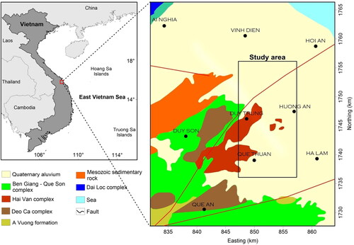
The northern Kontum massif is located in the northeastern part of the Indochina block and is one of the most key tectonic terranes of this block (Hung et al. 2020) (Figure 1). Studies on geological structures of an area can provide important information for understanding the evolutionary history of continental crust as well as tectonic environments. However, most of the region is covered by Quaternary alluvium, so deep geological structures of this region are not exposed (Figure 1). It is well known that such structures can be detected by using magnetic data (e.g. Pham et al. 2020; Pham, Eldosouky, et al. 2022; Pham, Oksum, Le, et al. 2022).

Figure 1. Geological map (UTM coordinates, zone 48 N) of the study area (Hieu et al. 2015). the faults reported by Phach and Anh (2018) are shown by the red lines.

This study aims to interpret aeromagnetic data of the northern Kontum massif (Vietnam) for mapping boundaries of subsurface geological sources using the tilt angle of the horizontal gradient (TAHG), improved theta map (ITM), horizontal gradient of the STDR (HGSTDR), fast sigmoid function (FSED), enhanced horizontal gradient amplitude (EHGA) and balanced horizontal gradient (BHG). Before applying these methods to real aeromagnetic data of the study area, it is necessary to estimate their effectiveness on synthetic examples. We also use the Source Parameter Imaging (SPI) and combined analytic signal and Euler (AN-EUL) methods to estimate the depths to the subsurface structures. The obtained result provides a first interpretation of the structural features of the northern Kontum massif.

2. Geological setting

The Kontum Massif is an outcropping structure located in the central part of Vietnam (Figure 1). The area is composed of sedimentary rocks corresponding to various periods, Paleozoic – Mesozoic magmatic rocks, early Paleozoic and Mesozoic metamorphic rocks and Precambrian rocks (Jiang et al. 2020). This massif is one of the major geological parts of the stable continental core of the Indochina terrane (Hutchison 1989). The Kontum massif compositions are the main high-grade metamorphic rocks (Nam et al. 2001; Nam, Osanai, Nakano 2004; Nam, Osanai, Nakano, et al. 2004). Figure 1 shows the geological map of the northern part of the Kontum massif and the location of the study area. The faults reported by Phach and Anh (2018) are also shown in this map. As can be observed, most of the northern part of the Kontum massif is covered by recent sediments. The region can be divided into four complexes: Hai Van, Ben Giang–Que Son, Dai Loc, and Deo Ca (Hieu et al. 2015). Most of the formations in the study area are NE-SW trending (Figure 1). The dominating formation is Quaternary alluvium. From SE to NW the order of the geological units is Hai Van granitoid, Ben Giang-Que Son complex, Deo Ca complex and Mesozoic sedimentary rock formations (Hieu et al. 2015). Therein, the Hai Van granitoid complex, with an exposed surface of thousands of square kilometers on the study map. The Hai Van granitoid complex is an important part of the northern Kontum massif and is composed of cordierite-bearing granitoid (Nakano et al. 2013), granodiorite, biotite granite, aplite two-mica granite, and granite (Thuc and Trung 1995). The granitoid rocks could be the products of different processes of tectonic processes, such as rift environments, orogenic activities, or from the mixed interaction between continental crust and mantle (Barbarin 1999; Li et al. 2014; Yang, Chen, et al. 2014; Yang, Long, et al. 2014).

3. Data and methods

3.1. Data

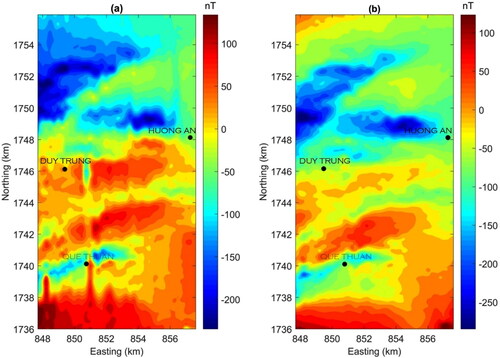
High-resolution aeromagnetic surveys can be used to determine geological structures in the Earth’s crust (Hang et al. 2019; Eldosouky, Pham, Abdelrahman, et al. 2022; Eldosouky, Pham, Abdelrahman, et al. 2022; Ghomsi, Kana, et al. 2022). In recent years, many digital magnetic datasets covering different geological regions have become available in Vietnam. Aeromagnetic data used in this study were collected from 1991 to 1994 by the Department of Geology and Minerals of Vietnam. The aircraft flight height was lower than 100 m. The total magnetic intensity (TMI) of magnetic data was deduced by subtracting the International Geomagnetic Reference Field (IGRF). Bogusz et al. (2014) recommend for data interpolation using the Kriging method with the variogram model run in the Surfer as it allows for the computation of errors in the interpolated data. This method is also known as a global interpolation method, and it minimizes the distortion of the interpolated field (Bogusz et al. 2014). For this reason, TMI aeromagnetic data are interpolated with a 100 m grid spacing using the Kriging method with default parameters within Surfer software (Version 13). The resulting aeromagnetic map is shown in Figure 2a. The aeromagnetic map (Figure 2a) represents the magnetic response from the local upper crustal geology (Dentith 2011; Oyeniyi et al. 2023) of the study area. The data set varies from −234 to 150 nT and the anomalies show a dominant E-W anomaly trend in the map. As can be seen from Figure 2a, negative anomalies are observed in the northern region of the study area, while positive anomalies are found in the southern region of the area. Since most of the northern part of the Kontum massif is covered by sediments, tectonic movement and lithological variations might be the reason for the variation of the magnetic field. The data for the interpretation should be taken from the RTP (reduction to the pole) or RTE (reduction to the equator) maps as the total magnetic intensity anomaly is not located exactly above the sources, which would lead to misinterpretation after applying the methods.

Figure 2. (a) Aeromagnetic anomaly map of the study area, (b) reduced-to-equator (RTE) aeromagnetic anomaly map of the study area.

3.2. Methods

3.2.1. Reduction to the equator (RTE)

The RTE has been proposed to process the magnetic anomaly at low latitudes instead of RTP. The RTE operator can be written as (Kis 1990; Hao et al. 2018): (1) $$L=-\frac{{\left[\cos (D-\theta )\right]}^2}{{\left[\mathrm{icos}\left(I\right)\cos \hspace{0.17em}\left(D-\theta \right)+\sin \left(I\right)\right]}^2},$$(1) where $\theta$ is the wavenumber direction, I is the magnetic inclination and D is the magnetic declination.

3.2.2. Edge enhancement methods

The TAHG is introduced by Ferreira et al. (2013) to map the source edges. The method is defined as the arctangent of the ratio of the derivatives of the horizontal gradient, and is given by: (2) $$\mathit{TAHG}=\mathit{atan}\frac{\frac{\partial HG}{\partial z}}{\sqrt{{\left(\frac{\partial HG}{\partial x}\right)}^2+{\left(\frac{\partial HG}{\partial y}\right)}^2}},$$(2) where $\frac{\partial HG}{\partial x},$ $\frac{\partial HG}{\partial y}$ and $\frac{\partial HG}{\partial z}$ are the derivatives of the horizontal gradient of the field F in the x, y and z directions, respectively, which is defined by: (3) $$HG=\sqrt{{\left(\frac{\partial F}{\partial x}\right)}^2+{\left(\frac{\partial F}{\partial y}\right)}^2,}$$(3) where $\frac{\partial F}{\partial x}$ and $\frac{\partial F}{\partial y}$ are the derivatives of the potential field in the x and y directions, respectively.

The method provides the maxima over the boundaries of the geological structures. The theoretical models of Ferreira et al. (2013) demonstrated that this method is less sensitive to the depth and that it can provide the source boundaries accurately.

The ITM is introduced by Chen et al. (2017) to improve the theta map method in mapping the source edges. The method is based on high order gradients of potential field anomalies, and is given as (Chen et al. 2017): (4) $$\mathit{ITM}=\mathit{acos}\frac{\sqrt{{\left(\frac{{\partial }^{2}F}{\partial z\partial x}\right)}^2+{\left(\frac{{\partial }^{2}F}{\partial z\partial y}\right)}^2}}{{\left(\frac{{\partial }^{2}F}{\partial z\partial x}\right)}^2+{\left(\frac{{\partial }^{2}F}{\partial z\partial y}\right)}^2+{\left(\frac{\partial F}{\partial z}/\left(p\times h\right)\right)}^2},$$(4) where $\frac{\partial F}{\partial z}$ is the vertical derivative of the field F, $\frac{{\partial }^{2}F}{\partial z\partial x}$ and $\frac{{\partial }^{2}F}{\partial z\partial y}$ are the derivatives of the vertical derivative, h is grid spacing, and p is a user-defined parameter that ranges from 0.05 to 5 (Chen et al. 2017). This method provides the minimum values over the edges of the geological structures.

Nasuti et al. (2019) introduced the HGSTDR method which is based on a combination of the second-order vertical derivative and the gradient of the gradient amplitude. The method is defined by: (5) $$\mathit{HGSTDR}=\sqrt{{\left(\frac{\partial \mathit{STDR}}{\partial x}\right)}^2+{\left(\frac{\partial \mathit{STDR}}{\partial y}\right)}^2},$$(5) where $\frac{\partial \mathit{STDR}}{\partial x}$ and $\frac{\partial \mathit{STDR}}{\partial y}$ are the derivatives of the STDR in the x, y and z directions, respectively, which is defined by: (6) $$\mathit{STDR}=\mathit{atan}\frac{M\times \frac{{\partial }^{2}F}{\partial z^2}}{\sqrt{{\left(\frac{\partial HG}{\partial x}\right)}^2+{\left(\frac{\partial HG}{\partial y}\right)}^2}},$$(6) with M is absolute magnetic value of the study region. The maxima of the HGSTDR are located over the source boundaries (Nasuti et al. 2019).

The FSED is introduced by Oksum et al. (2021) to map the edges of magnetic and gravity data. The method is based on the fast sigmoid function and derivatives of the gradient amplitude, and is given by: (7) $$\mathrm{FSED}=\frac{\mathrm{R}-1}{1+\left|\mathrm{R}\right|},$$(7) where (8) $$\mathrm{R}=\frac{\frac{\partial \mathrm{HG}}{\partial \mathrm{z}}}{\sqrt{{\left(\frac{\partial \mathrm{HG}}{\partial \mathrm{x}}\right)}^2+{\left(\frac{\partial \mathrm{HG}}{\partial \mathrm{y}}\right)}^2}}.$$(8)

The BHG is another balanced technique that uses the maximum values to map the boundaries of the potential field sources. This method is based on the derivatives of the gradient amplitude, which is given by (Prasad et al. 2022b): (9) $$\mathit{BHG}=\mathit{atan}\left(\frac{(k-1)\frac{\partial HG}{\partial z}-\left(k+1\right)\times \sqrt{{\left(\frac{\partial HG}{\partial x}\right)}^2+{\left(\frac{\partial HG}{\partial y}\right)}^2}}{\left|(k-1)\frac{\partial HG}{\partial z}-\left(k+1\right)\times \sqrt{{\left(\frac{\partial HG}{\partial x}\right)}^2+{\left(\frac{\partial HG}{\partial y}\right)}^2}\right|}\right),$$(9)

Another technique for mapping the edges of magnetic sources is presented by Pham, Eldosouky, et al. (2022), which uses the inverse sine function and the ratio of the derivatives of the gradient amplitude. The technique is given by: (10) $$\mathit{EHGA}=\mathcal{ }\mathcal{R}\left(\mathrm{asin}\left(k\left(\frac{\frac{\partial HG}{\partial z}}{\sqrt{{\left(\frac{\partial HG}{\partial x}\right)}^2+{\left(\frac{\partial HG}{\partial y}\right)}^2+{\left(\frac{\partial HG}{\partial z}\right)}^2}}-1\right)+1\right)\right),$$(10) where k ≥ 2 (Pham, Eldosouky, et al. 2022; Pham, Oksum, Kafadar, et al. 2022). The peaks in the EHGA map are located over the source boundaries.

3.2.3. SPI method

The SPI method (Thurston and Smith 1997) uses the local wavenumber to estimate multiple source parameters assuming a tabular (2D) model, but was designed to process gridded data. The local wavenumber is defined as: (11) $$k=\frac{\frac{{\partial }^{2}F}{\partial x\partial z}\frac{\partial F}{\partial x}+\frac{{\partial }^{2}F}{\partial y\partial z}\frac{\partial F}{\partial y}+\frac{{\partial }^{2}F}{\partial z^2}\frac{\partial F}{\partial z}}{{\left(\frac{\partial F}{\partial x}\right)}^2+{\left(\frac{\partial F}{\partial y}\right)}^2+{\left(\frac{\partial F}{\partial z}\right)}^2}.$$(11)

Thurston and Smith (1997) noted that, for a sloping contact, the peaks of $k$ are located over the edges of the contact, and its depth $h$ is calculated by the following equation: (12) $$h=\frac{1}{k_{\max }}.$$(12)

The local dip and susceptibility can also be determined in the absence of remanent magnetism.

3.2.4. AN-EUL method

The AN-EUL is based on a combination of the analytic signal and Euler methods (Salem and Ravat 2003). According to Salem and Ravat (2003), the top depth $h$ of a sloping contact is calculated by the following equation: (12) $$h=\frac{AS}{\mathit{EAS}},$$(12) where AS is the analytic signal that is given by (Roest et al. 1992): (13) $$AS=\sqrt{{\left(\frac{\partial F}{\partial x}\right)}^2+{\left(\frac{\partial F}{\partial y}\right)}^2+{\left(\frac{\partial F}{\partial z}\right)}^2},$$(13) and EAS is the enhanced analytic signal, and is expressed as (Hsu et al. 1996): (14) $$\mathit{EAS}=\sqrt{{\left(\frac{{\partial }^{2}F}{\partial z\partial x}\right)}^2+{\left(\frac{{\partial }^{2}F}{\partial z\partial y}\right)}^2+{\left(\frac{{\partial }^{2}F}{\partial z^2}\right)}^2}.$$(14)

We have implemented the above techniques as scripts for use in the MATLAB software, version R2017a or above.

3.2.5. Application of the enhancement techniques to synthetic data

Since each enhancement technique has its advantages and disadvantages, in this section we examine the effectiveness of the TAHG, ITM, HGSTDR, FSED, EHGA and BHG on synthetic magnetic data at the magnetic equator with and without noise. Figure 3a shows the 3D view of a synthetic model. The model includes two prisms located at different depths. The parameters of the model are given in Table 1. The magnetic anomalies of the model were calculated at 201 × 201 grid nodes with 250 m spacing (Figure 3b) using the method of Rao and Babu (1991). Figure 4a displays the result obtained from the TAHG method. As can be observed, the method can detect all the edges of the two prisms, but its signals are diffuse. Figure 4b displays the result determined from the ITM method. As can be seen, the method provides sharper responses over the edges than the TAHG, but it is less effective in mapping the south-north edges. Figure 4c shows the result obtained from the HGSTDR method. Clearly, the method shows a very high resolution for the determined boundaries. However, it is noteworthy that the ITM and HGSTDR generate some false boundaries in output maps Figure 4d–f shows the edges estimated by the FSED, EHGA and BHG methods, respectively. One can see that these methods bring sharper boundaries over the sources than the TAHG method. By comparing the obtained results from the six methods, it can see that all of them are effective in imaging the anomalies with different amplitudes, but the TAHG, FSED, EHGA and BHG do not generate secondary edges in the output results.

Figure 3. (a) Synthetic model, (b) magnetic anomaly of the model, (c). Gaussian random noise. Dashed lines show the true edges.

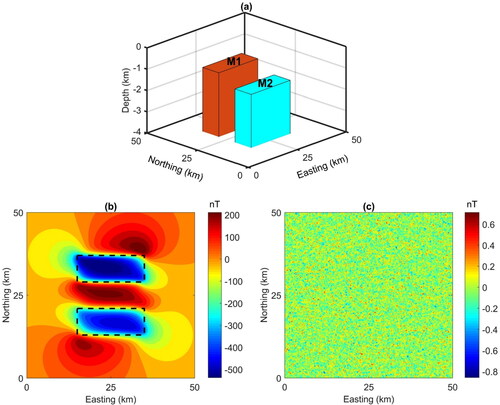
Figure 4. Enhanced maps of the noise-free synthetic data (Figure 3a): (a) TAHG, (b) ITM, (c) HGSTDR, (d) FSED, (e) EHGA, (f) BHG. Dashed lines show the true edges.

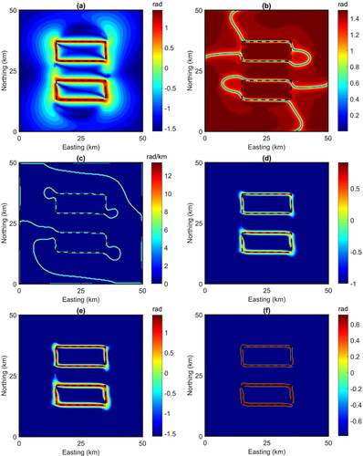
Table 1. Parameters of the synthetic model.

Parameters	M1	M2
x-coordinates of center (km)	25	25
y-coordinates of center (km)	33	17
Width (km)	8	8
Length (km)	20	20
Depth (km)	1	1.5
Declination (°)	25	25
Inclination (°)	0	0
Magnetization (A/m)	2	2

To further estimate the performance of the enhancement techniques, we consider a noisy example. Magnetic data in Figure 3a was corrupted with Gaussian noise (Figure 3b) having a standard deviation of 0.2 nT. Here, the noise was generated by using the ‘randn’ function in Matlab. Similar to the previous example, we also applied enhancement techniques to noise-corrupted data. Figure 5a–f displays the maps produced by the TAHG, ITM, HGSTDR, FSED, EHGA and BHG methods, respectively. As can be seen from these figures, the edges of two prisms are detected by all the TAHG, FSED, EHGA and BHG methods. Although the ITM and HGSTDR methods have sharper variations over the detected edges, they do not show the south-north edges. In addition, the results showed that the main disadvantage of the enhancement techniques is that they amplify the noise. However, it is noteworthy that the TAHG, FSED, EHGA and BHG are less sensitive to noise than the ITM and HGSTDR methods. In this case, with the use of upward continuation of magnetic data, the noise effect can be reduced (Nasuti et al. 2019).

Figure 5. Enhanced maps of the noise-free synthetic data (Figure 3b): (a) TAHG, (b) ITM, (c) HGSTDR, (d) FSED, (e) EHGA, (f) BHG. Dashed lines show the true edges.

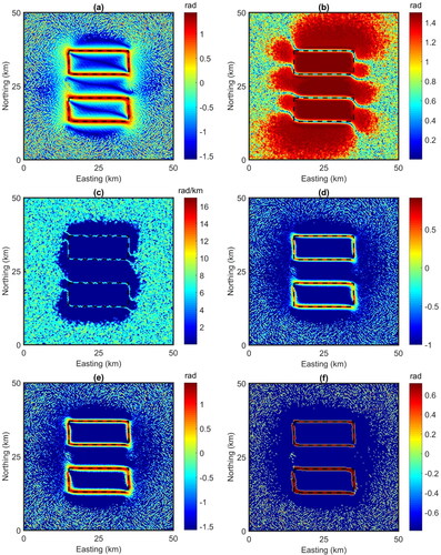
Based on the results of the synthetic data examples, it can be concluded that the ITM and HGSTDR can provide sharper responses over the edges than the TAHG, FSED, EHGA and BHG. However, the TAHG, FSED, EHGA and BHG are effective in mapping all edges without false information. In addition, the FSED, EHGA and BHG can bring the edges with higher resolution compared to the TAHG.

4. Results

Before applying the enhanced methods to the magnetic anomalous field, we assess the Earth’s magnetic field over the study area. The inclination (21.12°) and declination (−1.48°) of the study area were determined from International Geomagnetic Reference Field (IGRF) using coordinates at the center of the area. Since the inclination of the study area is quite low, the reduction to the pole (RTP) technique becomes notoriously unstable, resulting in several linear artifacts along the direction of magnetic declination. For this reason, the best solution is to reduce aeromagnetic data to the equator (Aina, 1986; Reford et al. 2010). Reduction to the equator (RTE) is required to symmetrize and center magnetic anomalies over the source bodies for better interpretation at low latitudes (Leu, 1986). Figure 2b shows RTE aeromagnetic data of the study area. The RTE data varies from −285 to 150 nT, and is dominated by E-W and ENE-WSW anomaly trends. The magnetic signature in the RTE map shows anomalies of different wavelengths and amplitudes, denoting the different magnetic contents of the causative bodies. As can be observed from Figure 2b, the RTE result is reasonable as it does not produce linear artifacts, therefore, it can be used to map the subsurface structures of the area.

Figure 6a–d displays the results obtained from applying the TAHG, ITM, HGSTDR, FSED, EHGA and BHG methods to RTE aeromagnetic data in Figure 2b, respectively. It can be seen that the methods clearly improved the magnetic anomaly signatures, which are not noticeably observed from the aeromagnetic data map in Figure 2b. However, since aeromagnetic data usually contain noise that is amplified by using the enhancement techniques, the results obtained from the methods are quite complex, especially for the ITM and HGSTDR. For this reason, the effect of noise should be first reduced. To solve this issue, an upward continuation filter can be applied to RTE aeromagnetic data.

Figure 6. Enhanced maps of the RTE aeromagnetic data (Figure 2b): (a) TAHG, (b) ITM, (c) HGSTDR, (d) FSED, (e) EHGA, (f) BHG.

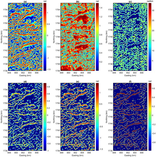
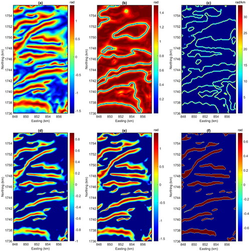
Figure 7a shows RTE aeromagnetic data after an upward continuation of 100 m. Figure 8a–f shows the results obtained from the application of the TAHG, ITM, HGSTDR, FSED, EHGA and BHG methods to upward-continued RTE aeromagnetic data in Figure 7a, respectively. In this case, all methods provide clearer images for the subsurface geological boundaries. In general, there is a good correlation among magnetic boundaries determined from the methods. It can be observed that the ITM and HGSTDR show sharper anomalies than the TAHG. However, the boundaries in the ITM and HGSTDR maps are connected, making it difficult to map real geological structures. The results of the TAHG, FSED, EHGA and BHG methods are quite similar, but the FSED, EHGA and BHG methods have been able to provide a clearer representation of structural boundaries and lithological contacts in the study area. The FSED, EHGA and BHG maps show sharper anomalies than those from the TAHG map. In this case, the small sources in the HGSTDR map are so prevalent, which may be related to noise. These sources provide less significant structural information, and bring a geological picture more complex than it is.

Figure 7. Upward continuation maps of the RTE aeromagnetic data (Figure 2b): (a) 100 m, (b) 500 m.

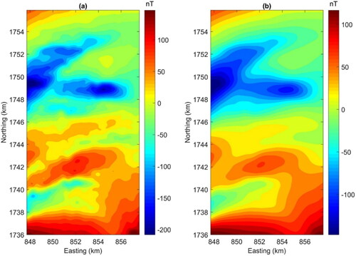
Figure 8. Enhanced maps of the 100 m upward continued aeromagnetic data (Figure 7a): (a) TAHG, (b) ITM, (c) HGSTDR, (d) FSED, (e) EHGA, (f) BHG.

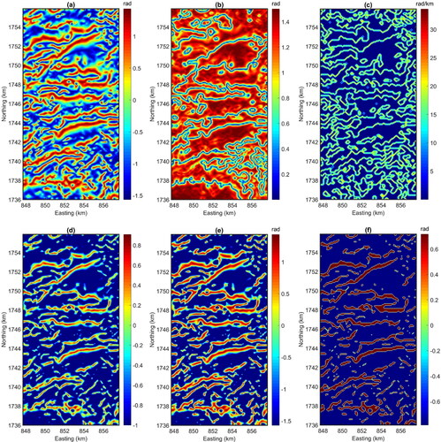
To further reduce the noise effect, we proceed to apply upward continuation filter to RTE aeromagnetic data to a height of 500 m. Figure 7b shows RTE aeromagnetic data after an upward continuation of 500 m. It can be seen that the resulting map is smoother than 100 m upward continued data, but the primary shapes of the magnetic field remain (Figures 2a and 7a,b). Figure 9a–f displays the results determined from the application of the TAHG, ITM, HGSTDR, FSED, EHGA and BHG methods to the upward-continued RTE aeromagnetic data in Figure 7b, respectively. Since the noise level is significantly reduced with a 500 m upward continuation filter, the results in Figure 9a–f is quite similar. The boundaries obtained from 500 m upward continued data correspond to the major geological structures in the area. Here, the ITM provides less information on the subsurface structures than the TAHG, HGSTDR, FSED, EHGA and BHG methods. Although the HGSTDR brings sharpened responses, it tends to connect magnetic edges. As shown in the synthetic examples, the ITM and HGSTDR filter allows for accurate estimations of the source edges, but they may generate secondary edges. In this case, the subsurface geological features are recognizable by the TAHG, and they are better displayed by the FSED, EHGA and BHG methods greatly improving the obtained results.

Figure 9. Enhanced maps of the 500 m upward continued aeromagnetic data (Figure 7b): (a) TAHG, (b) ITM, (c) HGSTDR, (d) FSED, (e) EHGA, (f) BHG.

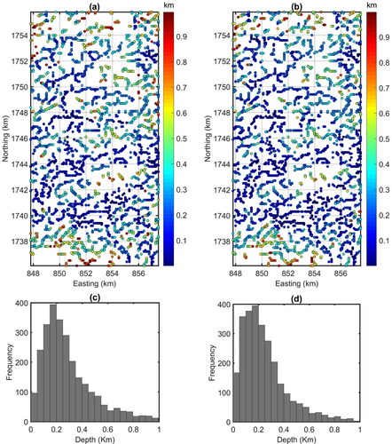
For further analysis, the SPI and AN-EUL methods were applied to the 100 m upward continued RTE aeromagnetic data to better describe the subsurface geological structures and find out how deep they are. Here, the peaks of $k$ and AS located over the edges of the contact are estimated by the Blakely and Simpson (1986) method. Figure 10a,b shows the solutions of the SPI and AN-EUL methods, respectively. As can be seen from these figures, the SPI result compares very favorably with the depth estimated by the AN-EUL method. Figure 10c,d displays the histograms of the depth solutions from the SPI and AN-EUL methods, respectively. It can be seen, the depths for most of the subsurface structures range from 50 to 550 m with an average depth of 250 m.

Figure 10. (a) the depths to the magnetic sources obtained by the SPI method, (b) the depths to the magnetic sources obtained by the an-EUL method, (c) Histogram of the SPI depths, (d) Histogram of the an-EUL depths.

5. Discussions

The synthetic study and processing of aeromagnetic data of the northern Kontum massif demonstrate that the ITM, HGSTDR, TAHG, FSED, EHGA and BHG are effective in balancing anomalies with the different amplitudes. The reason is that these methods are based on the ratios of derivatives of magnetic data. This equalizing effect is useful in the study area where magnetic anomalies have a large dynamic range and the magnetic map are dominated by the large amplitude anomalies with the E-W and ENE-WSW trends. However, no single method is a best tool for geological boundary identification; an integrated approach is always extremely helpful for superior correlation and assessment to provide more realistic information in the study area. With the help of the above studies including the ITM, HGSTDR, TAHG, FSED, EHGA and BHG analysis, the derived results are strongly correlate to each other solutions. Although the ITM and HGSTDR can provide structural boundaries in very high resolution, they bring false edge information as previously pointed out by Pham et al. (2021), Eldosouky et al. (2022) and Liu et al. (2023). The results on synthetic and real data also showed that the TAHG, FSED, EHGA and BHG are effective in avoiding bringing some false edges, but the FSED, EHGA and BHG generate sharper structural boundaries compared to the TAHG. In addition, since the upward continuation filter behaves like a low pass filter that transforms the measured data at an observation plan to another plan with a higher height (Mastellone et al. 2014; Zhang et al. 2018), the application of the FSED, EHGA and BHG to upward continued data map (Figures 8d–f and 9d–f) are less noisy than the FSED, EHGA and BHG of RTE aeromagnetic data map (Figure 6d–f). For these reasons, the lineaments in the study region were extracted from the FSED, EHGA and BHG maps of upward continued data (Figures 8d–f and 9d–f), and are shown in Figure 11a–c.

Figure 11. Magnetic lineaments from upward-continued data with height 100 m (black lines) and 500 m (red lines), superimposed on the SPI solutions (a), an-EUL solutions (b) and 100 m upward-continued RTE data (c), structural map of the study area, inferred from aeromagnetic data interpretation (d). probable granitic intrusions are also marked as grey areas.

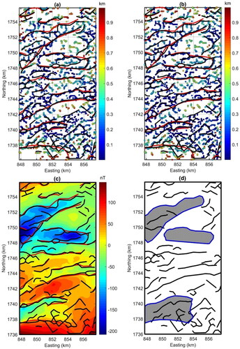
For further validation of the subsurface structural boundaries determined by the enhancement filters, the SPI and AN-EUL solutions were superimposed on the magnetic lineaments (Figure 11a,b). As can be seen from these figures, the estimated magnetic boundaries match with many SPI and AN-EUL solutions. In addition, the structural features generated at heights of 100 and 500 m show the E-W and ENE-WSW trends similar to the RTE anomalies (Figure 11c). They suggest that most of magnetic sources in northern part of the Kontum massif are the deep-level buried structures. This information agrees with the information found in the geological studies where the Quaternary sediments cover most of the area (Hieu et al. 2015; Faure et al. 2018; Jiang et al. 2020). Moreover, one can see that there is a strong correlation between the magnetic lineaments of 100 m upward continued data and those of 500 m upward continued data. While the lineament map of 500 m upward continued data provides horizontal locations of the major structures in the area, the lineament map of 100 m upward continued data can map both major and smaller structures, being the small structures related to shallower sources. The TAHG maps (Figures 8a and 9a) also confirm the existence of the FSED, EHGA and BHG lineaments, but with a lower resolution; while and the ITM and HGSTDR results (Figures 8b,c and 9b,c) show a good correlation with these lineaments. Figure 11d shows the subsurface structural map of the northern Kontum massif derived from magnetic interpretation. It can be seen that a variety of lineaments was identified in Figure 11d with the dominance of the E-W and ENE-WSW orientations. The horizontal locations of the obtained SPI and AN-EUL solutions also confirm the existence of these lineaments. The E-W trending lineaments may be the result of the collision between the North and the South Vietnam blocks (Faure et al. 2018). The age of the collision remains uncertain, although it is generally considered as Triassic (Faure et al. 2018). The SE movement of the Indosinian geoblock probably resulted in the formation of the ENE-WSW trending lineaments. Due to this movement, the southern part of Central Vietnam became a frontal tectonic zone where the Indosinian geoblock contacted the East Vietnam Sea terrain via a N‐S trending fault (Phach and Anh 2018). Therefore, the studies over the southern part of Central Vietnam and adjacent areas can clarify the tectonic evolution of the area, especially the processes of formation and development of the East Vietnam Sea.

Magnetic gradients commonly occur where geological edges have juxtaposed rocks of different susceptibilities. However, geological edges are not always marked by magnetic gradients, as rocks of similar susceptibilities may be juxtaposed along an edge or rocks do not contain a significant amount of magnetic material. Most of the study area is covered by sediments. The surface geology map only shows the Hai Van granitoid complex. Based on zircon U–Pb ages and geochemical data, Hieu et al. (2015) reported that the Hai Van granitoid complex (Figure 1) is composed of peraluminous rocks that have chemical characteristics of S-type granites with high SiO₂, Na₂O + K₂O, and Zr contents as well as typical S-type minerals such as cordierite and muscovite. On the other hand, it is well known that non-magnetic granites usually correspond to supracrustal sources, S-type, where iron is fractionated mainly in ilmenite (paramagnetic at room temperature) and biotite (strongly paramagnetic) (Chappell and White 2001; Pueyo et al. 2022). For this reason, the edges obtained from magnetic interpretation do not match with the boundaries of the Hai Van granitoid complex in the study area.

As stated by Nagy et al. (2001), the Kontum massif is an uplifted block of high-grade metamorphic rocks, and it is intruded by granitic bodies. This interpretation also reveals the presence of intrusive structures with their boundaries highlighted by blue lines in Figure 11d. It is well known that anomalies over high magnetization bodies are negative at the equator because of a 180° phase transition from the poles to the equator. Here, the intrusive structures are also verified by the RTE anomaly map (Figure 11c) where their boundaries are located over negative anomalies. The SPI depth solutions provide deeper depths to the eastern and northeastern parts of the area whilst shallower ones occupy the eastern part. That seems to represent the northeastern and eastern extension of the magnetic structures in the subsurface. The obtained result in Figure 11d compares favorably with the fault reported by Phach and Anh (2018) (Figure 1). The composite lineaments map (Figure 11d) also indicates that the subsurface of the study area is heavily dissected by linear geological structures, some of which are probably faults in the subsurface. These faults may be the result of the pre-spreading extension of the continental lithosphere, as pointed out by Huu Nguyen et al. (2022). Clearly, the FSED, EHGA and BHG techniques are able not only to balance weak and strong magnetic amplitudes, but also to reveal interesting geological features without connected lineaments (Figure 11d). The extraction of the network of magnetic boundaries using the FSED, EHGA and BHG techniques technique allows us to propose a first structural map for the study area; which shows a network of lineaments hidden under the Quaternary sediments, and such structures are not identified by geological studies (i.e. Rangin et al. 1995; Lan et al. 2003; Tran et al. 2014. Hieu et al. 2015; Faure et al. 2018; Shang and Chen 2022). This result provides some references for further research within geological aims in the northern part of the Kontum massif.

6. Conclusions

Aeromagnetic data of the northern part of the Kontum massif have been interpreted using the recent methods such as the tilt angle of the horizontal gradient (TAHG), improved theta map (ITM), horizontal gradient of the STDR (HGSTDR), fast sigmoid function (FSED), enhanced horizontal gradient amplitude (EHGA) and balanced horizontal gradient (BHG), Source Parameter Imaging (SPI) and combined analytic signal and Euler (AN-EUL) methods. The interpretation allowed us to distinguish the anomalies from structures of different magnetizations, then draw the map of geological structures hidden under the Quaternary sediments in the area. These findings provide a variety of lineaments with a dominance of the E-W and ENE-WSW oriented trends. The E-W may be the result of the collision between the North and the South Vietnam blocks, while the ENE-WSW trending lineaments are related to the SE movement of the Indosinian plate. The results also show the extension of the magnetic structures to the east and northeast in the northern part of the Kontum massif. This study provided the first aeromagnetic data interpretation for a better understanding of the subsurface geological structures of the northern Kontum massif.

Acknowledgments

Deep thanks and gratitude to the Researchers Supporting Project number (RSP2023R249), King Saud University, Riyadh, Saudi Arabia, for funding this research article. This paper is a contribution to TNMT.2022.02.20 ‘Developing technology to interpret magnetic and gravity data (satellite/airborne/ground data) to identify buried geological structures for investigation and assessment of deep mineral resources in Vietnam’ from Ministry of Natural Resources and Environment, Vietnam. S. P. Oliveira thanks the National Council of Technological and Scientific Development [CNPq, 316376/2021-3]. The authors would like to thank the regional editor Dr Rundquist and three anonymous reviewers for their comments and recommendations.

Disclosure statement

No potential competing interest was reported by the author(s).

Data availability statement

The data that support the findings of this study are available from the corresponding author, upon reasonable request.

Correction Statement

This article has been corrected with minor changes. These changes do not impact the academic content of the article.

References

- Aina AO. 1986. Reduction to equator, reduction to pole and orthogonal reduction of magnetic profiles. Explor Geophys. 17(3):141–145. doi: 10.1071/EG986141.
- Barbarin B. 1999. A review of the relationships between granitoid types, their origins and their geodynamic environments. Lithos. 46(3):605–626. doi: 10.1016/S0024-4937(98)00085-1.
- Blakely R, Simpson R. 1986. Approximating edges of source bodies from magnetic or gravity anomalies. Geophysics 51(7):1494–1498. doi: 10.1190/1.1442197.
- Bogusz J, Kłos A, Grzempowski P, Kontny B. 2014. Modelling the velocity field in a regular grid in the area of Poland on the basis of the velocities of European permanent stations. Pure Appl Geophys. 171(6):809–833. doi: 10.1007/s00024-013-0645-2.
- Catalán M, Martín Davila J. 2003. A magnetic anomaly study offshore the Canary Archipelago. Mar Geophys Res. 24(1-2):129–148. doi: 10.1007/s11001-004-5442-y.
- Castro FR, Oliveira SP, de Souza J, Ferreira FJF. 2020. Constraining Euler deconvolution solutions through combined tilt derivative filters. Pure Appl Geophys. 177(10):4883–4895. doi: 10.1007/s00024-020-02533-w.
- Chappell BW, White AJ. 2001. Two contrasting granite types: 25 years later. Aust J Earth Sci. 48(4):489–499. doi: 10.1046/j.1440-0952.2001.00882.x.
- Chen AG, Zhou TF, Liu DJ, Zhang S. 2017. Application of an enhanced theta-based filter for potential field edge detection: a case study of the Luzong ore district. Chin J Geophys. 60(2):203–218.
- Cooper GRJ, Cowan DR. 2006. Enhancing potential field data using filters based on the local phase. Computers & Geosciences. 32(10):1585–1591. doi: 10.1016/j.cageo.2006.02.016.
- Cordell L, Grauch VJS. 1985. Mapping basement magnetization zones from aeromagnetic data in the San Juan Basin, New Mexico. In: Hinze WJ, editor. The utility of regional gravity and magnetic maps. 1st ed. Tulsa (OK): society of Exploration Geophysicists; p. 181–197.
- Dentith M. 2011. Magnetic methods, airborne. In: Gupta HS, editor. Encyclopedia of solid earth geophysics. Vol. 1. Dordrecht: Springer; p. 761–766. doi: 10.1007/978-90-4818702-7_119.
- Ekinci YL, Ertekin C, Yiğitbaş E. 2013. On the effectiveness of directional derivative based filters on gravity anomalies for source edge approximation: synthetic simulations and a case study from the Aegean graben system (western Anatolia, Turkey). J Geophys Eng. 10(3):035005. doi: 10.1088/1742-2132/10/3/035005.
- Ekwok SE, Eldosouky AM, Ben UC, Alzahrani H, Abdelrahman K, Achadu OIM, Pham LT, Akpan AE, Gómez-Ortiz D. 2022. Application of high-precision filters on airborne magnetic data: a case study of the Ogoja Region, Southeast Nigeria. Minerals. 12(10):1227. doi: 10.3390/min12101227.
- Eldosouky AM, Pham LT, Mohmed H, Pradhan B. 2020. A comparative study of THG, AS, TA, Theta, TDX and LTHG techniques for improving source boundaries detection of magnetic data using synthetic models: a case study from G. Um Monqul, North Eastern Desert, Egypt. J Afr Earth Sci. 170:103940. doi: 10.1016/j.jafrearsci.2020.103940.
- Eldosouky AM, Pham LT, Abdelrahman K, Fnais MS, Gomez-Ortiz D. 2022. Mapping structural features of the Wadi Umm Dulfah area using aeromagnetic data. J King Saud Univ Sci. 34(2):101803. doi: 10.1016/j.jksus.2021.101803.
- Eldosouky AM, Pham LT, Duong VH, Ghomsi FEK, Henaish A. 2022. Structural interpretation of potential field data using the enhancement techniques: a case study. Geocarto Int. 37(27):16900–16925. doi: 10.1080/10106049.2022.2120548.
- Eldosouky AM, Pham LT, Henaish A. 2022. High precision structural mapping using edge filters of potential field and remote sensing data: a case study from Wadi Umm Ghalqa area, South Eastern Desert, Egypt. Egypt J Remote Sens Space Sci. 25(2):501–513. doi: 10.1016/j.ejrs.2022.03.001.
- Essa KS, Nady AG, Mostafa MS, Elhussein M. 2018. Implementation of potential field data to depict the structural lineaments of the Sinai Peninsula, Egypt. J Afr Earth Sci. 147:43–53. doi: 10.1016/j.jafrearsci.2018.06.013.
- Faure M, Nguyen VV, Hoai LTT, Lepvrier C. 2018. Early Paleozoic or Early-Middle Triassic collision between the South China and Indochina Blocks: the controversy resolved? Structural insights from the Kon Tum massif (Central Vietnam). J Asian Earth Sci. 166:162–180. doi: 10.1016/j.jseaes.2018.07.015.
- Fedi M, Florio G. 2001. Detection of potential fields source boundaries by enhanced horizontal derivative method. Geophysical Prospecting. 49(1):40–58. doi: 10.1046/j.1365-2478.2001.00235.x.
- Ferreira FJF, de Souza J, de Bongiolo A, de Castro LG. 2013. Enhancement of the total horizontal gradient of magnetic anomalies using the tilt angle. Geophysics. 78(3):J33–J41. doi: 10.1190/geo2011-0441.1.
- Ghomsi FEK, Pham LT, Tenzer R, Esteban FD, Vu TV, Kamguia J. 2022. Mapping of fracture zones and structural lineaments of the Gulf of Guinea passive margins using marine gravity data from CryoSat-2 and Jason-1 satellites. Geocarto Int. 37(25):10819–10842.
- Ghomsi FEK, Pham LT, Steffen R, Ribeiro-Filho N, Tenzer R. 2022. Delineating structural features of North Cameroon using EIGEN6C4 high-resolution global gravitational model. Geol J. 57(10):4285–4299.
- Ghomsi FEK, Kana JD, Aretouyap Z, Ribeiro-Filho N, Pham LT, Baldez R, Tenzer R, Mandal A, Nzeuga A. 2022. Main structural lineaments of the southern Cameroon volcanic line derived from aeromagnetic data. J Afr Earth Sci. 186:104418. doi: 10.1016/j.jafrearsci.2021.104418.
- Hinze WJ, Frese RRB, Saad AH. 2013. Gravity and magnetic exploration: principles, practices, and applications. New York: Cambridge University Press; p. 1–525.
- Hang NTT, Oksum E, Minh LH, Thanh DD. 2019. An improved space domain algorithm for determining the 3-D structure of the magnetic basement. Vietnam J Earth Sci. 41(1):69–80. doi: 10.15625/0866-7187/41/1/13550.
- Hao M, Zhang F, Tai Z, Du W, Ren L, Li Y. 2018. Reduction to the pole at low latitudes by using the Taylor series iterative method. J Appl Geophys. 159:127–134. doi: 10.1016/j.jappgeo.2018.08.004.
- Hung NQ, Thanh NX, Dao VD. 2020. U-Pb ages of zircon from I- and S-type granites from northern Kon Tum terrane: implications for late Paleozoic - Mesozoic magmatism in Central Vietnam. J Geol Soc Korea. 56(6):727–735.
- Hieu PT, Yang YZ, Binh DQ, Nguyen TBT, Dung LT, Chen F. 2015. Late Permian to Early Triassic crustal evolution of the Kontum massif, central Vietnam: zircon U–Pb ages and geochemical and Nd–Hf isotopic composition of the Hai Van granitoid complex. Int Geol Rev. 57(15):1877–1888. doi: 10.1080/00206814.2015.1031194.
- Hutchison CS. 1989, Geological evolution of South-east Asia: Oxford monographs on geology and geophysics 13, Oxford: Clarendon Press.
- Huu Nguyen H, Carter A, Hoang LV, Fox M, Pham SN, Vinh HB. 2022. Evolution of the continentalmargin of south to central Vietnam andits relationship to opening of the SouthChina Sea (East Vietnam Sea). Tectonics. 41(2):e2021TC006971. doi: 10.1029/2021TC006971.
- Hsu S, Sibuet J, Shyu C. 1996. High-resolution detection of geologic boundaries from potential field anomalies: an enhanced analytic signal technique. Geophysics. 61(2):373–386. doi: 10.1190/1.1443966.
- Ibraheem IM, Aladad H, Alnaser MF, Stephenson R. 2021. TAS: a new novel phase-based filter for detection of unexploded ordnances. Remote Sensing. 13(21):4345. doi: 10.3390/rs13214345.
- Ibraheem IM, Tezkan B, Ghazala H, Othman AA. 2023. A new edge enhancement filter for the interpretation of magnetic field data. Pure Appl Geophys. 180(6):2223–2240. doi: 10.1007/s00024-023-03249-3.
- Jiang W, Yu JH, Wang X, Griffin WL, Pham T, Nguyen D, Wang F. 2020. Early Paleozoic magmatism in northern Kontum Massif, Central Vietnam: insights into tectonic evolution of the eastern Indochina Block. Lithos. 376-377:105750. doi: 10.1016/j.lithos.2020.105750.
- Joel ES, Olasehinde P I, Adagunodo TA, Omeje M, Akinyemi ML, Ojo JS. 2019. Integration of aeromagnetic and electrical resistivity imaging for groundwater potential assessment of coastal plain sands area of Ado-Odo/Ota in Southwest Nigeria. Groundw Sustain Dev. 9:100264. doi: 10.1016/j.gsd.2019.100264.
- Jorge VT, Saulo Pomponet Oliveira SP, Luan Thanh Pham LT, Van-Hao Duong VH. 2023. A balanced edge detector for aeromagnetic data. Vietnam J Earth Sci. 43(3):326–337. doi: 10.15625/2615-9783/18461.
- Kis KI. 1990. Transfer properties of the reduction of magnetic anomalies to the pole and to the equator. Geophysics. 55(9):1141–1147. doi: 10.1190/1.1442930.
- Kamto PG, Oksum E, Pham LT, Kamguia J. 2023. Contribution of advanced edge detection filters for the structural mapping of the Douala Sedimentary Basin along the Gulf of Guinea. Vietnam J Earth Sci. 43(3):287–302. doi: 10.15625/2615-9783/18410.
- Kumar S, Pal SK, Guha A, Sahoo SD, Mukherjee A. 2022. New insights on Kimberlite emplacement around the Bundelkhand Craton using integrated satellite-based remote sensing, gravity and magnetic data. Geocarto Int. 37(4):999–1021. doi: 10.1080/10106049.2020.1756459.
- Kumar, U, Pal, SK, Sahoo, SD, Narayan, S, Mondal, S, Ganguli, SS, Saurabh. 2018. Lineament mapping over sir creek offshore and its surroundings using high resolution EGM2008 gravity data: an integrated derivative approach.J Geol Soc India. 91(6):671–678. doi: 10.1007/s12594-018-0922-x.
- Lan CY, Chung SL, Van Long T, Lo CH, Lee T Y, Mertzman SA, Shen JJS. 2003. Geochemical and Sr–Nd isotopic constraints from the Kontum massif, central Vietnam on the crustal evolution of the Indochina block. Precambrian Res. 122: 7–27. doi: 10.1016/S0301-9268(02)00205-X.
- Ma G, Li L. 2012. Edge detection in potential fields with the normalized total horizontal derivative. Comput. Geosci. 41:83–87. doi: 10.1016/j.cageo.2011.08.016.
- Mastellone D, Fedi M, Ialongo S, Paoletti V. 2014. Volume continuation of potential fields from the minimum-length solution: an optimal tool for continuation through general surfaces. J Appl Geophys. 111:346–355. doi: 10.1016/j.jappgeo.2014.10.020.
- Miller HG, Singh V. 1994. Potential field tilt a new concept for location of potential field sources. J Appl Geophys. 32(2-3):213–217. doi: 10.1016/0926-9851(94)90022-1.
- Leu L. 1986. Magnetic exploration with reduction of magnetic data to the equator. (U.S. Patent No. 4,570,122). U.S. Patent and Trademark Office
- Li S-Q, Hegner E, Yang Y-Z, Wu J-D, Chen F. 2014. Age constraints on late Mesozoic lithospheric extension and origin of bimodal volcanic rocks from the Hailar basin, NE China. Lithos. v. 190-191:204–219. doi: 10.1016/j.lithos.2013.12.009.
- Liu J, Li S, Jiang S, Wang X, Zhang J. 2023. Tools for edge detection of gravity data: comparison and application to tectonic boundary mapping in the Molucca Sea. Surv Geophys. doi: 10.1007/s10712-023-09784-x.
- Nabighian MN, Grauch VJS, Hansen RO, LaFehr TR, Li Y, Peirce JW, Phillips JD, Ruder ME. 2005. The historical development of the magnetic method in exploration. Geophysics. 70(6):33ND–61ND. doi: 10.1190/1.2133784.
- Nagy EA, Maluski H, Lepvrier C, Schärer U, Phan T T, Leyreloup A, Vu VT. 2001. Geodynamic significance of the Kontum massif in central Vietnam: composite 40Ar/39Ar and U–Pb ages from Paleozoic to Triassic. J Geol 109:755–770. doi: 10.1086/323193.
- Nakano N, Osanai Y, Owada M, Nam TN, Charusiri P, Khamphavong K. 2013. Tectonic evolution of highgrade metamorphic terranes in central Vietnam: constraints from large-scale monazite geochronology. J Asian Earth Sci. v. 73:520–539. doi: 10.1016/j.jseaes.2013.05.010.
- Nam TN, Osanai Y, Nakano N. 2004. Tectono-metamorphic evolution of crystalline basement complexes in the Kontum massif, Vietnam: fact and question? Gondwana Res. 7:1353–1355.
- Nam TN, Osanai Y, Nakano N, Tham HH. 2004. Permo-triassic ultrahigh-temperature metamorphism and continental collision in the Kon Tum massif. J Geol. 285:1–8. [In Vietnamese with English abstract].
- Nam TN, Sano Y, Terada K, Toriumi M, Quynh PV, Dung LT. 2001. First shrimp U–Pb zircon dating of granulites from the Kontum massif (Vietnam) and tectonothermal implications. J Asian Earth Sci. 19(1–2):77–84. doi: 10.1016/S1367-9120(00)00015-8.
- Narayan S, Sahoo SD, Pal SK, Kumar U, Pathak VK, Majumdar TJ, Chouhan A. 2017. Delineation of structural features over a part of the Bay of Bengal using total and balanced horizontal derivative techniques. Geocarto Int. 32(4):351–366. doi: 10.1080/10106049.2016.1140823.
- Nasuti Y, Nasuti A, Moghadas D. 2019. STDR: a novel approach for enhancing and edge detection of potential field data. Pure Appl Geophys. 176(2):827–841. doi: 10.1007/s00024-018-2016-5.
- Oksum E, Le DV, Vu MD, Nguyen THT, Pham LT. 2021. A novel approach based on the fast sigmoid function for interpretation of potential field data. Boll Geofis Teor Appl. 62:543–556.
- Oladejo OP, Adagunodo TA, Sunmonu LA, Adabanija MA, Enemuwe CA, Isibor PO. 2020. Aeromagnetic Mapping of fault architecture along Lagos-ore axis, Southwestern Nigeria. Open Geosciences. 12(1):376–389. doi: 10.1515/geo-2020-0100.
- Oladejo OP, Adagunodo TA, Sunmonu LA, Adabanija MA, Olasunkanmi NK, Omeje M, Babarimisa IO, Bility H. 2019. Structural analysis of subsurface stability using aeromagnetic data: a case of Ibadan, southwestern Nigeria. J Phys: conf Ser. 1299:012083. doi: 10.1088/1742-6596/1299/1/012083.
- Oyeniyi T, Akanbi TI, Falade AH. 2023. An application of softsign function (SF) filter to low-latitude aeromagnetic data of Tafawa-Balewa Area, Northern Nigeria for geostructural mapping and tectonic analysis. Res Geophys Sc. 14:100063. doi: 10.1016/j.ringps.2023.100063.
- Phach PV, Anh LD. 2018. Tectonic evolution of the southern part of Central Viet Nam and the adjacent area. Geodin Tektonofiz. 9(3):801–825. doi: 10.5800/GT-2018-9-3-0372.
- Pham LT, Eldosouky AM, Abdelrahman K, Fnais MS, Gomez-Ortiz D, Khedr F. 2021. Application of the improved parabola-based method in delineating lineaments of subsurface structures: a case study. J King Saud Univ Sci. 33(7):101585. doi: 10.1016/j.jksus.2021.101585.
- Pham LT, Minh LH, Oksum E, Thanh DD. 2018. Determination of maximum tilt angle from analytic signal amplitude of magnetic data by the curvature-based method. Vietnam J Earth Sci. 40(4):354–366. doi: 10.15625/0866-7187/40/4/13106.
- Pham LT, Oksum E, Do TD. 2019. Edge enhancement of potential field data using the logistic function and the total horizontal gradient. Acta Geod Geophys. 54(1):143–155. doi: 10.1007/s40328-019-00248-6.
- Pham LT, Oksum E, Do TD, Le-Huy M, Vu MD, Nguyen VD. 2019. LAS: a combination of the analytic signal amplitude and the generalised logistic function as a novel edge enhancement of magnetic data. Contributions to Geophysics and Geodesy. 49(4):425–440. doi: 10.2478/congeo-2019-0022.
- Pham LT, Vu TV, Le-Thi S, Trinh PT. 2020. Enhancement of potential field source boundaries using an improved logistic filter. Pure Appl Geophys. 177(11):5237–5249. doi: 10.1007/s00024-020-02542-9.
- Pham LT, Eldosouky AM, Oksum E, Saada SA. 2022. A new high resolution filter for source edge detection of potential field data. Geocarto Int. 37(11):3051–3068. doi: 10.1080/10106049.2020.1849414.
- Pham LT, Oksum E, Le DV, Ferreira FJF, Le ST. 2022. Edge detection of potential field sources using the softsign function. Geocarto Int. 37(14):4255–4268. doi: 10.1080/10106049.2021.1882007.
- Pham LT, Oksum E, Kafadar O, Trinh PT, Nguyen DV, Vo QT, Le ST, Do TD. 2022. Determination of subsurface lineaments in the Hoang Sa islands using enhanced methods of gravity total horizontal gradient. Vietnam J Earth Sci. 44(3):395–409.
- Pham LT, Prasad KND. 2023. Analysis of gravity data for extracting structural features of the northern region of the Central Indian Ridge. Vietnam J Earth Sci. 45(2):147–163.
- Pilkington M, Keating PB. 2009. The utility of potential field enhancements for remote predictive mapping. Can J Remote Sens. 35(sup1):S1–S11. doi: 10.5589/m09-021.
- Pilkington M, Tschirhart V. 2017. Practical considerations in the use of edge detectors for geologic mapping using magnetic data. Geophysics. 82(3):J1–J8. doi: 10.1190/geo2016-0364.1.
- Prasad KND, Pham LT, Singh AP. 2022a. A Novel Filter “ImpTAHG” for Edge Detection and a Case Study from Cambay Rift Basin, India. Pure Appl Geophys. 179(6-7):2351–2364. doi: 10.1007/s00024-022-03059-z.
- Prasad KND, Pham LT, Singh AP. 2022b. Structural mapping of potential field sources using BHG filter. Geocarto Int. 37(26):11253–11280. doi: 10.1080/10106049.2022.2048903.
- Pueyo EL, Román-Berdiel T, Calvín P, Bouchez JL, Beamud E, Ayala C, Loi F, Soto R, Clariana P, Margalef A, et al. 2022. Petrophysical characterization of non-magnetic granites; density and magnetic susceptibility relationships. Geosciences. 12(6):240. doi: 10.3390/geosciences12060240.
- Rangin C, Huchon P, Le Pichon X, Bellon H, Lepvrier C, Roques D, Hoe ND, Van Quynh P. 1995. Cenozoic deformation of central and south Vietnam. Tectonophysics. 251(1–4):179–196. doi: 10.1016/0040-1951(95)00006-2.
- Rao DB, Babu NR. 1991. A rapid method for three dimensional modeling of magnetic anomalies. Geophysics. 56(11):1729–1737. doi: 10.1190/1.1442985.
- Ravat D. 2007. Upward and downward continuation. In: Gubbins D, Herrero-Bervera E, editors. Encyclopedia of Geomagnetismand Paleomagnetism. Dordrecht: Springer; p. 974–976.
- Reford SW, Misener DJ, Ugalde HA, Gana JS, Oladele O. 2010. Nigeria’s nationwide high-resolution airborne geophysical surveys. SEG Denver 2010 annual meeting. Conference paper; p. 1835–1839.
- Roest WR, Verhoef J, Pilkington M. 1992. Magnetic interpretation using the 3D analytic signal. Geophysics. 57(1):116–125. doi: 10.1190/1.1443174.
- Saibi H, Mogren S, Mukhopadhyay M, Ibrahim E. 2019. Subsurface imaging of the Harrat Lunayyir 2007–2009 earthquake swarm zone, western Saudi Arabia, using potential field methods. J Asian Earth Sci. 169:79–92. doi: 10.1016/j.jseaes.2018.07.024.
- Salem A, Ravat D. 2003. A combined analytic signal and Euler method (AN‐EUL) for automatic interpretation of magnetic data. Geophysics. 68(6):1952–1961. doi: 10.1190/1.1635049.
- Salem A, Williams S, Fairhead J, Ravat D, Smith R. 2007. Tilt-depth method: a simple depth estimation method using first-order magnetic derivatives. Lead. Edge. 26(12):1502–1505. doi: 10.1190/1.2821934.
- Shang Z, Chen Y. 2022. Petrogenesis and Tectonic implications of early Paleozoic Magmatism in Awen Gold District, south section of the Truong Son Orogenic Belt, Laos. Minerals. 12(8):923. doi: 10.3390/min12080923.
- Stewart ICF, Miller DT. 2018. Directional tilt derivatives to enhance structural trends in aeromagnetic grids. J Appl Geophys. 159:553–563. doi: 10.1016/j.jappgeo.2018.10.004.
- Thompson DT. 1982. EULDPH: A new technique for making computer-assisted depth estimates from magnetic data. Geophysics. 47(1):31–37. doi: 10.1190/1.1441278.
- Thuc DD, Trung H. 1995. Vietnam geology, part of II: magma. Hanoi: Department of Geology and Mineral Resources Survey; p. 213–219. [In Vietnamese with English abstract]
- Thurston JB, Smith RS. 1997. Automatic conversion of magnetic data to depth, dip, and susceptibility contrast using the SPI (TM) method. Geophysics. 62(3):807–813. doi: 10.1190/1.1444190.
- Tran HT, Zaw K, Halpin JA, Manaka T, Meffre S, Lai CK, L HV, Dinh S. 2014. The Tam Ky-Phuoc Son shear zone in central Vietnam: tectonic and metallogenic implications. Gondwana Res. 26(1), 144–164. doi: 10.1016/j.gr.2013.04.008.
- Weihermann JD, Ferreira FJF, Oliveira SP, Cury LF, de Souza J. 2018. Magnetic interpretation of the Paranaguá terrane, southern Brazil by signum transform. J Appl Geophys. 154:116–127. doi: 10.1016/j.jappgeo.2018.05.001.
- Wijns C, Perez C, Kowalczyk P. 2005. Theta map: edge detection in magnetic data. Geophysics. 70(4):L39–L43. doi: 10.1190/1.1988184.
- Yang Y-Z, Chen F, Siebel W, Zhang H, Long Q, He J-F, Hou Z-H, Zhu X-Y. 2014. Age and composition of Cu–Au related rocks from the lower Yangtze River belt: constraints on paleo-Pacific slab roll-back beneath eastern China. Lithos. v202-203:331–346. doi: 10.1016/j.lithos.2014.06.007.
- Yang Y-Z, Long Q, Siebel W, Cheng T, Hou Z-H, Chen F. 2014. Paleo-Pacific subduction in the interior of eastern China: evidence from adakitic rocks in the EdongJiurui district. The Journal of Geology. 122(1):77–97. doi: 10.1086/674423.
- Yuan Y, Gao JY, Chen LN. 2016. Advantages of horizontal directional Theta method to detect the edges of full tensor gravity gradient data. J Appl Geophys. 130:53–61. doi: 10.1016/j.jappgeo.2016.04.009.
- Zhang C, Lü Q, Yan J, Qi G. 2018. Numerical solutions of the mean-value theorem: new methods for downward continuation of potential fields. Geophys Res Lett. 45(8):3461–3470. doi: 10.1002/2018GL076995.