Performance assessment of the Sentinel-2 LAI products and data fusion techniques for developing new LAI datasets over the high-altitude Himalayan forests

Abstract

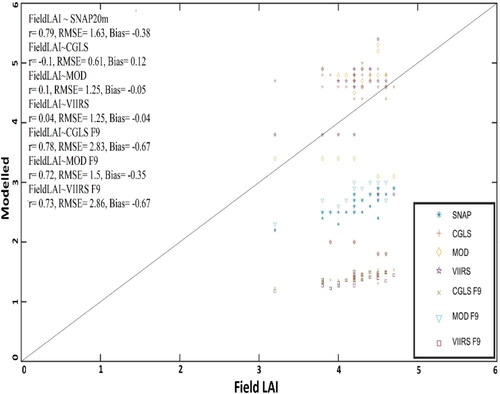
The present study evaluates the accuracy of SNAP-Sentinel-2 Prototype Processor (SL2P) derived Leaf Area Index (LAI) and proposes a new simple method to generate new datasets of LAI through data fusion. Rigorous optimization of the data fusion approaches (Kalman filter and Linear weighted) were performed for the generation of new LAI products over the complex hilly terrain of the Himalayan region. The results showed a good correlation (r = 0.79) and low error (RMSE = 1.63) between SNAP-derived (at 20 m) and ground-observed LAI. A lower correlation was obtained between the ground observed LAI data and the corresponding global LAI products for the Moderate Resolution Imaging Spectroradiometer (MODIS) (r = 0.1, RMSE = 1.19), Copernicus Global Land Service (CGLS) (r = 0.1, RMSE = 0.61) and the Visible Infrared Imaging Radiometer Suite (VIIRS) (r = 0.04, RMSE = 1.25). Notably, after implementing the data fusion, both SNAP-derived LAI and Global LAI products exhibited much-improved performance statistics with ground observed data sets.

Keywords:

• Leaf area index
• data fusion
• SNAP
• Himalayan forests
• Sentinel-2

Introduction

The identification and evaluation of forest biophysical parameters are very crucial in the current era of climate change. Such information can be used in a variety of applications and at different geographical scales, including land surface process monitoring, natural resource management, and hydrological modelling (Fang, Baret, et al. 2019; Fang, Zhang, et al. 2019). The Global Climate Observing System (GCOS) has included Leaf Area Index (LAI) as an important variable that can be retrieved from optical sensors onboard Earth-observing satellite platforms (Le Maire et al. 2008; Verrelst et al. 2019) and documented its importance in estimating leaf density, plant functioning, vegetation health, and biogeochemical cycles (Verger et al. 2016; Danner et al. 2021).

To comprehend the manner in which vegetation canopies engage with the surrounding environment, it is vital to possess an understanding of their leaf area (Bright et al. 2015) . The leaf area interacts with solar radiation to generate energy by regulating canopy gaseous exchanges. Consequently, it regulates stress levels, influences vegetation productivity, and impacts photosynthetic capacity (Boegh et al. 2013). Direct LAI measuring methods using in-situ approaches can be used, but they are costly, time-consuming, labor-intensive, and destructive in nature (Yan et al. 2016) and cover only a small geographical area. To overcome this limitation, remotely-sensed LAI retrieval can be used as an alternative to LAI measurements. In the last decades, a wide range of LAI retrieval methods have been proposed utilizing data acquired from satellite products. With the availability of many Earth Observation (ΕΟ) satellites, a variety of relevant LAI products at various spatiotemporal resolutions have now become available. Those include, for example, the MODIS (500 m, 4-day) (Yan et al. 2016), the CGLS (GEOV2, 1 km and 300 m, 10-day) Version 3 (Camacho et al. 2013), and the European Organization for the Exploitation of Meteorological Satellites (EUMETSAT) Polar System Satellite Application Facility (SAF EPS, 1.1 km, 10-day) (García-Haro et al. 2018), and the Global Land Surface Satellite (GLASS) (500 m, 8-day) (Xiao et al. 2016). It is clearly of key importance to conduct scientific validation of such available data products. This would assist in comprehending their accuracy and quantifying the errors associated with their predictions (Morisette et al. 2006). However, the applications of coarse-resolution LAI products created from MODIS, AVHRR, SPOT-VGT, and CGLS are limited and need to be alleviated. With high resolution Sentinel-2's satellite datasets, this issue can be addressed. Towards this end, the ESA’s SNAP toolbox offers great flexibility in performing atmospheric correction using the Sen2Cor tool as well as estimating biophysical parameters. This can be done using the physically based radiative transfer models PROSPECT leaf optical properties model and SAIL canopy bidirectional reflectance model (PROSAIL) (Jacquemoud and Baret 1990), with a machine learning approach, e.g. Neural Networks (NNs) (Xiao et al. 2016). Nevertheless, to our knowledge, few studies have so far looked at the validity of SL2P-derived LAI using Sentinel-2 (Simon Blessing 2019) over diverse and heterogeneous high-altitude forest ecosystems. Thus, it is evidently of critical importance that further studies be performed on this front since the reliability and inter-comparability of biophysical indicators like LAI need to be assessed for accurate and reliable forest monitoring (Morisette et al. 2006; Yan et al. 2016).

The Sentinel-2 constellation is the flagship EO satellite system of the Copernicus programme (Camacho et al. 2013; Knyazikhin et al. 2013; Verger et al. 2016). This massive data set has been useful for quantifying and monitoring vegetation features, with LAI being the most effective indicator of vegetation dynamics (Verger et al. 2011; García-Haro et al. 2018). Significant progress has been made in the availability of high-resolution, freely available space-borne datasets through sensors like Sentinel 2 and freely available software tools for processing, such as ESA’s SNAP. In addition, data fusion techniques provide an efficient way to produce high-quality datasets for different applications. Such approaches provide a strong means of combining the data and knowledge sources from two complimentary sensor types to create a consistent, accurate, and valuable representation of real-world scenarios (Srivastava et al. 2013; Joshi et al. 2016). Biophysical parameters, such as the LAI over highly heterogeneous landforms like the Himalayas need such methods to overcome data quality issues at various temporal and spatial scales. Various studies have reported a variety of data fusion methods. Those vary from simplistic Linear Weighted Algorithm (LWA) (Li et al. 2003) to complex Kalman filter (KF) (Sun 2004) along with Multiple Linear Regression (MLR) (Krzywinski and Altman, 2015) and Artificial Neural Network (ANN). Although there is a plethora of data fusion techniques available, there is indeed so far little information to help in choosing from them and how they improve the datasets (Pettorelli et al. 2018).

In the purview of the above, the present study employs two data fusion algorithms to establish a correlation between ground-observed LAI and Global LAI datasets. The first method is a Linear Weighted Algorithm and the second is Kalman Filter’s Simulated Annealing (SANN) method. Moreover, uncertainties concerning the effect of spatial resolution and data processing levels on derived biophysical parameters like LAI need additional examination, especially in highly heterogeneous mountainous ecosystems. Thus, the present study objective is 2-fold: (a) to perform a thorough evaluation of the SNAP-derived LAI from ground observations and global LAI products like MODIS, CGLS, and AVHRR sensors at the same time; and (b) to introduce a simple method to compare coarse-resolution LAI products with fine-scale Sentinel-2 LAI products. The proposed method uses ground LAI measurements, recalibrates Sentinel-2 LAI using the Committee on Earth Observation Satellites (CEOS) Land Product Validation (LPV) upscaling validation methodology, and provides optimized global datasets with ground measurements to develop high-quality LAI datasets.

Materials and methods

Study area

The field study was carried out in the lower Dachigam part of the Dachigam National Park (DNP), Srinagar, from 6 to 9 August 2021. DNP is situated in central Kashmir, in the western Himalayas. The DNP spans between 340.05″ and 340.10″ north latitude to 740.50″ and 750.10″ east longitude, at an elevation of 1600–4500 m above mean sea level. It covers an area of 141 square kilometers. The open scrubland type of vegetation is dominant here and covers roughly one-third of the total floral diversity (Shameem et al. 2010). The vegetation of Dachigam National Park, according to Kishore et al. (2020), is a typical Himalayan moist temperate forest.

In the lower portions of Dachigam, common shrub species are found, including Prunus, Rubus, Berberis, Vibernum, Rosa, Indigofera, and Parrotiopsis. At an elevation ranging from 3400 to 4100 m, Upper Dachigam is naturally rich with broad meadows that sustain lush herbaceous grass and perennial mesophytic flora. The area’s annual rainfall is around 2460 mm, and the temperature ranges from 3 to 23 °C. The weather in the Dachigam region is quite unpredictable. The annual maximum rainfall in Dachigam remains around 546 mm, with a low of 32 mm. In general, the climate stays sub-Mediterranean in nature, with two dry seasons in April-June and September-November (Figure 1).

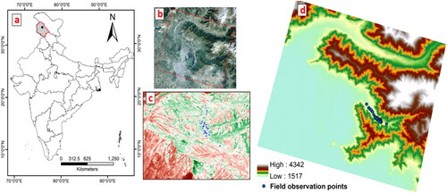
Figure 1. Location map of ground observation points in Dachigam National Park, Srinagar. (a) A country map showing the study location, (b) a natural colour image of the study area, (c) a 3-D view of the sampling site, and (d) an elevation map of the study area.

Field observed data and satellite-derived LAI

A LICOR 2200 C Plant Canopy Analyzer was used to collect in situ LAI datasets in 30 × 30 m plots in randomly selected 32 transects along the valley (Richardson et al. 2011). One reading that was taken above the canopy as a reference was done so in the open, outside of the measurement field (clear sky) and four readings that were taken below the canopy were done so at a height of ∼5 cm above the ground. These readings were taken randomly within each plot to reflect the variability of each plot. The PAIeff was calculated using the LAI-2200 following the Miller (1967) theorem (Miller 1967).

Sentinel-2 reflectance data

The Sentinel-2 mission is in the constellation and includes two identical satellites acquiring data at 13 spectral bands and at a spatial resolution of 10 m [blue, green, red, near-infrared (NIR) bands], 20 m [three vegetation red edge bands, a narrow NIR band, and two short-wave infrared (SWIR) bands], and 60 m (coastal aerosol, water vapour, and SWIR-Cirrus bands) with an average 5-day repeat cycle. The datasets of Sentinel-2 L2A [Bottom-of-Atmosphere (BOA) reflectance] covering the period from 1 August 2021 to 31 August 2021 were acquired with the least/no cloud cover from the Copernicus Open Access Hub (https://scihub.copernicus.eu/dhus/).

MODIS LAI

Every four days, the MODIS collection 6 (C6) LAI product (MCD15A3H) with a spatial resolution of 500 m is obtained from a combination of Terra MODIS and Aqua MODIS satellites. The fundamental technique for producing the MODIS LAI output is based on a three-dimensional radiative transfer model (3D-RTM) (Myneni et al. 2002) using lookup tables (LUTs). Because of the significant uncertainty in other bands, the programme only takes the red and NIR daily surface reflectance data (MOD09GA, 500 m) as input.

CGLS 300 m/GEOV3 LAI

The CGLS 300 m (also known as GEOV3) LAI was created by using PROBA-V data with a 10-day temporal resolution and a 300-m spatial resolution (Camacho et al. 2013; Verger et al. 2016). Like its predecessor, GEOV3 is based on the use of NNs trained to utilize fusions of the MODIS C5 and CYCLOPES v3.1 products, as was the case with GEOV2. Estimates of daily LAI were derived from the daily synthesis of PROBA-V reflectance in the blue, red, and near-infrared bands, as well as the view-sun geometry, which is performed using neural networks. Like GE-OV2, the daily estimates of LAI provided by the NNs were smoothed and temporally composited at a 10-day step to construct the final GEOV3 products. When comparing the GEOV2 and GEOV3 algorithms, the most significant difference is that the GEOV3 algorithm does not make use of climatology to fill in the gaps in the data.

LAI from VIIRS

The LAI and Fraction of Photosynthetically Active Radiation (FPAR) Version 1 data products from the Visible Infrared Imaging Radiometer Suite (VIIRS) offer information on the vegetative canopy layer at a resolution of 500 m (VNP15A2H). The VIIRS sensor is mounted on the Suomi National Polar-Orbiting Partnership (Suomi NPP) satellite, which is jointly operated by the National Oceanic and Atmospheric Administration (NOAA) and the National Aeronautics and Space Administration (NASA). To ensure the Earth Observation System (EOS) mission’s continuation, this product is modelled after the Terra and Aqua Moderate Resolution Imaging Spectroradiometer (MODIS) LAI/FPAR operating algorithm. Six Science Data Set Layers are included in the VNP15A2H package for analyzing significant parameters in LAI/FPAR measurements. The LAI and FPAR measurements, as well as the quality detail for LAI/FPAR, extra quality detail for FPAR, and the standard deviation for LAI and FPAR are all included.

Methodology

Validation of model derived LAI and reference map generation

The ‘Biophysical Processor’ in SNAP is used to prepare LAI products with a spatial resolution of 10 and 20 m (in the ‘Thematic Land Processing’ pulldown menu). Using RTMs like PROSAIL and the NNs method in the Biophysical Processor, the LAI, Canopy Water Content (CWC), Canopy Chlorophyll Content (CCC), fPAR, and Fraction of Vegetation Cover (FVC) can be retrieved from the Sentinel-2 TOA images. In the processor, along with the zenith and azimuth angles, a total of eight reflectance bands ranging from B3 to B8(8A) and B11 to B12 were used. A spectral measure known as the Directional Area Scattering Factor (DASF) was used to estimate the percentage of leaf area visible from a specific direction inside the canopy (Knyazikhin et al. 2013). It is monotonically correlated with LAI and foliage clumping and ranges from zero to one with no dimensions (Stenberg and Manninen 2015; Adams et al. 2018). The SNAP-derived LAI was rescaled and co-registered using the nearest neighbour resampling approach. The detailed process can be found in Brown et al., 2021.

Field-to-satellite data product comparison

The coarse-resolution LAI products were directly compared against ground-observed LAI data. Such validation studies largely rely on field-observed data sets obtained from a small region or single location. The points must be representative of the satellite pixel area or satellite overpass (Fang, Zhang, et al. 2019). The geographic mismatch between the standard decametric LAI, hectometric and ground-observed datasets needs to be sorted out before validation. The geo-mismatch and footprint impact were reduced by averaging out all of the LAI values in the given pixel. This significantly decreases the samples number while also increasing the reliability with temporal differences of under 8 days to reduce the temporal mismatch impact.

Comparison of global LAI products with upscaled, high-resolution reference datasets

To overcome the scale gaps between ground data and coarse resolution pixels of satellite data products, the field-observed LAI was scaled up to coarse scale pixels via the fine resolution sentinel 2 LAI product. The upscaling process was performed using a transfer function that links the field observed LAI to the high-resolution reflectance from satellite imagery (Baret et al. 2006; Morisette et al. 2006). SNAP-based Sentinel-2 LAI was the first product to be validated and further upscaled at the resolution of coarse-scaled LAI data products. Recalibrating the SL2P-based Sentinel-2 LAI product by using a linear regression against the ground observed data and then compared directly with coarse scaled data by up-scaling the SNAP-derived LAI using the SNAP rescale function, which is shown to be more accurate. The upscaling was done by using the nearest neighbour approach (Figure 2).

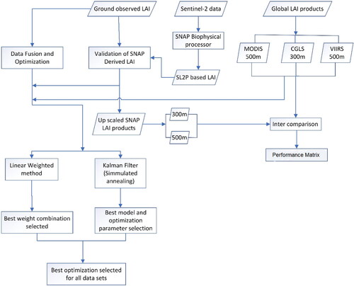
Figure 2. Flowchart of the methodology employed in this study.

Data fusion and optimization

For further improvement and large-scale retrieval of LAI at high spatial resolution, data fusion techniques were attempted. Before opting to use the data-fusion methods, an exhaustive parameterization must be performed. Changing series weights from 0 to 1 are taken into consideration in the LWA technique, which is used for model selection and parameter tuning. Such approaches based on trial and error are used rather frequently in selecting the optimal value of the parameter in linear weighted data fusion algorithms.

Linear weighted algorithm (LWA)

This Linear Weighted Algorithm (LWA) is also called as weighted sum method. The weights for input variables are determined first in the linear combination method. The input variables values were then multiplied by the weights obtained earlier. The best weight combination is determined by a series of values ranging from 0 to 1 and then keeping a 0.1 interval, the weighting values for both variables are changed in such a way that the total sum remains as 1. After that, using the weighted sum process, the best-performing weight combination is selected for data fusion. The equation is defined as: (1) $$\mathit{LWA}=\mathrm{ }\sum _{i=1}^n(w_1\times x_i+w_2\times y_i)$$(1) where, w₁ and w₂ = weight coefficients (w₁ + w₂ should be = 1), n = total number of values.

The field LAI is represented by the x_i and subsequent SNAP-derived and global LAI datasets are represented by y_i, respectively.

Kalman filter

State space models provide a reliable framework for modelling various kinds of time series and other data. Statistical models like ARIMA, structural time series, simple regression, GLM, and cubic spline smoothing may be termed state space models. Dynamic linear models are considered the simplest type of state space models and are often used in various scientific problem-solving because of their analytically tractable behaviour.

With discrete time intervals t = 1, …, n, and continuous state space, in the Gaussian state space model, we have (2) $$y_t= Z_t{\alpha }_t+ {\in }_t\mathrm{ }\left(\text{Observational equation}\right)$$(2) (3) $${\alpha }_{t+1}=\mathrm{ }{T}_t{\alpha }_t+\mathrm{ }{R}_t{\eta }_{t }\left(\text{State equation}\right)$$(3) (4) $${\alpha }_{t+1}=E\left({\alpha }_{t+1}\mathrm{yt},\dots ,\mathrm{y}1\right)$$(4) (5) $${\upsilon }_t=\mathrm{ }yt\text{-}\mathrm{ }{Z}_t{\alpha }_t$$(5)

Where, $y_t$ = observations at time t, ${\alpha }_t$ = vector of the latent state process at time t, Z_t, T_t, and R_t (system matrices) together with H_t and Q_t (covariance matrices) are time invariable (do not depend on t) but depend on the model definition.

The Kalman filtering and smoothing, the two recursive algorithms are used to know the latent state α for the given observations y. The covariance matrices, prediction error, and the one-step-ahead predictions are obtained from the Kalman filtering algorithms. (6) $$P_{t+1}=\mathit{VAR}\left({\alpha }_{t+1}|yt,\dots ,y1\right)$$(6) (7) $$F_t=\mathrm{ }\mathit{VAR}\left({\upsilon }_t\right)=\mathrm{ }{Z}_t{P}_t{Z}_t^{\mathrm{T}}+\mathrm{ }{H}_t$$(7)

The state smoothing equations running backwards in time and yielding can be established by using the results of the Kalman filtering (Durbin and Koopman 2013). (8) $$\widehat{{\alpha }_t}=E\left({\alpha }_{t+1}|y_n,\dots ,y1\right)$$(8) (9) $$V_t=\mathit{VAR}\left({\alpha }_{t+1}|y_n,\dots ,y1\right)$$(9)

All Kalman Filter and Smoother for Exponential Family State Space (KFAS) functions use Koopman and Durbin’s univariate approach (Koopman and Durbin 2003; Durbin and Koopman 2013), also called sequential processing (Anderson and Moore 1979).

When considering the Kalman filter, each function makes use of a univariate method, which is also referred to as sequential processing. The results are both faster and more consistent because KFAS does not need matrix inversion and only takes one observation at a time. In the present study, the best linearization for the Kalman solution was obtained after 1,000,000 iterations. The univariate approach introduces observations one at a time, because, the process uses no matrix inversion, in this case, to approximate a singular error variance matrix denoted as F and F_inf were used. By adding disturbances to the state vector or LDL decomposition on H, the model can be modified if the H is not diagonal (if necessary, it is done automatically in KFAS).

Simulated annealing (SANN)

The SANN method under the Kalman filter approach is a version of the simulated annealing given in Bélisle (1992) and comes under the family of stochastic global optimization methods. It is a method for handling optimization problems that are both unconstrained and bound-constrained. It uses a statistical mechanics approach to locate global optima in systems. The acceptance probability of this method is calculated using the Metropolis function. (10) $$S=\mathrm{ }\frac{1}{1+\exp \left(\frac{\Delta }{\max T}\right)}$$(10)

Where, T = Current variable of interest

This probability is likewise determined by a parameter T, here, T is a variable in an annealing system. The algorithm is similar to hill climbing, except it chooses a random move instead of the optimum one. If the chosen move improves the solution, it is always approved, or, the algorithm will make the move with a probability of <1 in any case. Uphill movements are more common with higher T values, they grow increasingly implausible, as T approaches 0, until the algorithm mimics the hill climbing. T decreases subsequently according to an ‘annealing schedule’ from a high start point in a normal SANN optimization. Using a simulated annealing method, a new point is generated at random at the beginning of each cycle. A probabilistic distribution is used to determine the distance between the current point and the new point. The algorithm prevents itself from becoming stuck in a local minimum by accepting all locations that raise the objective. This enables the algorithm to explore broadly for additional possible solutions rather than being constrained to a single location.

Performance evaluation matrix

Three statistical metrics were used to measure the goodness-of-fit, accuracy, and systematic deviation, namely the correlation coefficient (R), Root Mean Square Error (RMSE), and Bias. The maximum uncertainty level (0.5, 20%) that was given by GCOS was used as a benchmark to determine the quality of LAI estimated through different methods.

Results

Comparison of SNAP-derived LAI with ground-observed LAI

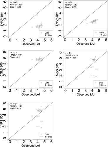
In this study, it was used the SNAP-derived LAI from Sentinal-2 data using an SL2P biophysical processor. SNAP-derived LAI at 20 m spatial resolution demonstrated a similar trend as of ground observed data and was in good agreement with ground observed LAI, with R = 0.79 and bias = −0.38. At the same time, it shows a higher error value of RMSE = 1.63. But despite being finer resolution, the 10 m LAI product does not show a good relationship with ground observed LAI with r = 0.49, bias = −0.58, and high RMSE = 2.45 (Figures 3 and 4). Figure 3(c) shows the differential LAI estimation over high-altitude forest areas and agriculture and pasture lands.

Figure 3. Sentinal-2 SNAP derived LAI products (a,b) at 10 and 20 m and (c) difference map Similarly, global LAI products were tested using ground-observed datasets. All the global LAI products considered in the present study performed poorly over the study region.

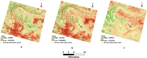
Figure 4. Scatterplots showing relationships between (a,b) observed LAI and SL2P derived LAI (at 10 and 20 m), (c–e) observed LAI and global LAI products (MODIS_500 m, CGLS_300 m, and VIIRS_500 m).

Intercomparison of SNAP LAI with global LAI products

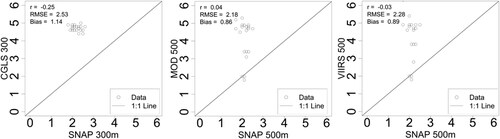
SNAP-derived LAI was compared with MODIS, VIIRS, and CGLS LAI products to determine the consistency and compatibility. Global LAI products do not show a good consistency with SNAP-derived up-scaled LAI products, especially at higher spatial resolution. The correlation and RMSE values were found very high for MODIS (0.04, 2.18) and VIIRS-derived LAI (0.03, 2.28) at 500 m resolution when compared with the ground datasets. CGLS shows a slightly better correlation with r = 0.25 and but a high RMSE (2.53) was obtained (Figure 5).

Figure 5. Scatter plot showing the relationship between upscaled (at 300 and 500 m) SL2P-derived LAI products and global coarse LAI products (MODIS_500 m, CGLS_300 m, and VIIRS_500 m).

Table 1 summarizes the statistical results of the R and RMSE that concerning the comparisons among the derived and global LAI products. The performance matrix shows the strength of the relationship among ground observed, SNAP derived, and global LAI product data. Yet, the SNAP-derived LAI products at various spatial resolutions and their upscaled products do not demonstrate a very satisfactory agreement with a global product at the same scale.

Table 1. Performance evaluation matrix.

	Field_LAI-S2_10	Field_LAI-S2_20	Field_LAI-CGLS_300	Field_LAI-MOD500	Field_LAI-VIIRS_500	S2_up_300-CGLS_300	S2_up_500-MOD_500	S2_up_300-VIIRS_500
R	0.49	0.79	0.1	0.1	0.04	0.25	0.04	0.03
RMSE	2.45	1.63	0.61	1.19	1.25	2.53	2.18	2.28
Bias	−0.58	−0.38	0.12	−0.05	−0.04	1.14	0.86	0.89

Optimization of global products

As shown in the previous section, a clear correlation between ground-observed LAI and Sentinel-2-derived LAI is evident and ascertains its relationship with global coarse resolution LAI product datasets. Changing series weights from 0 to 1 are taken into consideration in the LWA technique, which is used for model selection and parameter tuning. The results of testing the functionality of various data sets using a variety of weight combinations are given in Supplementary Data (S1). The best weight combination for the individual data type is shown using the Taylor diagram in Figure 6. The weight combination 0.1 for ground observed LAI and 0.9 for the global LAI products, shows the best result. At 0.1–0.9 weight combination the MODIS LAI product shows the highest correlation with r = 0.78 (Figure 7).

Figure 6. Taylor plot showing best performing tuned parameter of linear weighted algorithm optimization for (a) CGLS LAI product, (b) MODIS LAI product, and (c) VIIRS LAI product.

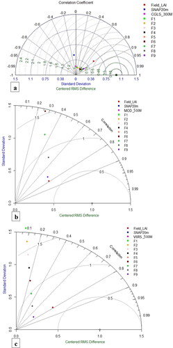
Figure 7. LAI dataset performance with LWA optimization (scatter plot with 1:1 equiline).

The data shows that all the global products underestimate before the data fusion. After linear weighted optimization all the global data sets are now showing a good correlation with the ground observed LAI and validated SNAP-derived LAI product data (Figure 7).

In the present study, the best linearization for the Kalman solution is obtained after 1,000,000 iterations. To optimize global data sets with ground-observed LAI, the SANN algorithm which is a stochastic global optimization method is used. To estimate the log-likelihood of a non-Gaussian state-space object the values for independent variables were tried at every possible combination (0–>1) and (0.7–0.9) combination was used because it works for all the global LAI product taken into account in the present study. The results of testing the functionality of various data sets using a variety of weight combinations are given in Supplementary Data (S2). The best weight combination for the individual data type is shown using the Taylor diagram in Figure 8.

Figure 8. Taylor plot showing best performing tuned parameter of Kalman Filter (SANN) algorithm optimization for (a) CGLS LAI product, (b) MODIS LAI product, and (c) VIIRS LAI product.

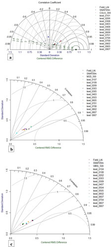
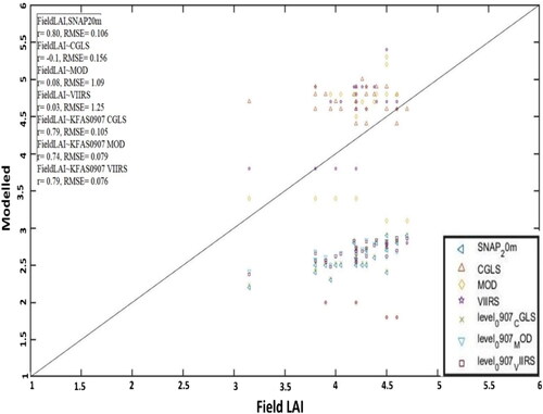
Also, at this, all the global LAI product showed a good correlation with the ground datasets. CGLS and VIIRS are both showed good agreement after optimization with r = 0.79 (Figure 9).

Figure 9. LAI dataset performance with Kalman filter optimization (scatter plot with 1:1 equiline).

The overall performance of the two optimization techniques with non-fused datasets reveals that the data fusion techniques can significantly improve the forest biophysical parameter for large-scale forest management and policy planning.

Discussion

The Dachigam National Park in the Himalayan which was chosen as the study area in this study is a very heterogenous area and high variations can be seen due to changing topology with elevation. Fine-resolution Sentinel-2 datasets present a good opportunity for fine-scale biophysical parameter estimation over highly biodiverse regions. The bio-physical processor makes it more convenient to estimate the vegetation parameters with in-built LUT and machine learning-based algorithms. Most of the validation studies for SL2P-derived LAI were carried out over croplands and homogenous forest types, when it comes to highly heterogeneous landscapes like the Indian Himalayan region, the ground validation of such fine-scale products becomes very complicated. In the present study, the SNAP-derived LAI products at 10 m resolution showed good to moderate consistency with the field observed datasets.

SNAP-derived 20 m LAI product showed a satisfactory relationship with ground datasets, though there is a higher degree of heterogeneity at the local scale in the Himalayan region exists, which makes it tough to validate fine scale products. This can be understood by the comparisons between ground observed and well-established course resolution global LAI products. The 20 m LAI product from Sentinel-2 did not have a good agreement with global datasets (Figure 4). When SNAP-derived 20 m LAI product was upscaled to the global LAI product datasets, no significant improvement in the relationship with the global products was obtained. MODIS LAI products showed a lower agreement with the SNAP-derived upscaled LAI products than Copernicus CGLS LAI. When compared with the SNAP-derived upscaled LAI products, MODIS LAI had a modest square of correlation and CGLS has a comparatively stronger square of correlation than the SNAP-derived upscaled LAI products. This could be explained by the difference in the algorithmic design and input factors that are used for SNAP-derived LAI and global LAI products. For instance, the MODIS LAI approach is tailored to a particular biome and makes use of LUTs built with 3D RTMs. The first key finding is that, when compared to in-situ LAI data, SNAP-derived LAI correlates relatively well, however, the inaccuracies are statistically significant. It was discovered that LAI values calculated by the SNAP were overestimated, with accuracy varying depending on topography and sparse vegetation. A second key finding of the present study is that the spatial resolution of the SNAP-derived LAI affects its performance; the disparity in accuracy that exists between the various SNAP-derived upscaled LAI data and global LAI products is an example of this issue. Yet, it should be noted that the present study findings are not in agreement with other studies, such as those reported by Hu et al. (2020), which though were performed in dissimilar experimental settings. Third, SNAP-derived LAI does not match up with global LAI products, although the errors between MODIS LAI and CGLS LAI are statistically significantly distinct from one another. In the absence of improved calibration in the current biophysical processor method, this reveals its limited applicability over the Himalayan region.

Variables that are input include the structural type of the vegetation, the geometry of the sensor, the BRFs at red (648 nm) and NIR (858 nm), as well as the accompanying uncertainties (Yin et al. 2017). Due to the low resolution, there is a possibility that the plant type per pixel of interest might be misclassified. The latter could lead to an error when compared to the data from Sentinel-2, which has a higher resolution (Mayr and Samimi 2015). In contrast, the Biophysical processor (i.e. S2LP) is comparable to the CGLS LAI algorithm in the sense that both are based on ANN and include a larger number of input variables. However, in the Himalayan environment, the poor training sample integration into the SNAP biophysical processor continues to be the primary challenge. Despite the bio-physical processor incorporating additional factors, such as visible, RE, NIR, and SWIR bands, the relationship between the LAI simulated using the SNAP was of lower agreement in comparison to the global ones. This is due to the fact that the SNAP-derived LAI is more sensitive to changes in LAI than the global LAI products are (Jin et al. 2017). In addition, it’s possible that the higher dimensionality of the input in the SNAP biophysical processor is to blame for the greater inaccuracies that exist between the SNAP-derived LAI and the global LAI products (De Kauwe et al. 2011; Brown et al. 2020). As a consequence of this, the primary focus of study in the years to come should be on determining the optimal subset of variables for enhancing the LAI estimation.

A pixel obtained from a higher resolution sensor is likely to comprise a generally uniform land cover, whereas a pixel in a lower resolution image may encompass a broad array of land cover types and demonstrate significant variability (Wu and Li 2009). The variance in spatial heterogeneity is the major component driving the geographical scale effects influencing the accuracy of LAI estimation and validation (Wu et al. 2016). The high RMSE in SNAP calculated LAI and ground observed LAI (RMSE = 1.63) could be due to this. The RMSE increases significantly as we get towards lower resolution data, as shown in numerous earlier research. Nonetheless, the occurrence of spatial heterogeneity is controlled by factors, such as plant canopy size, canopy heterogeneity, and terrain (Frazer et al. 2005; Zhang et al. 2015; Denny and Nielsen 2017). The current study region is diverse in canopy size and structure, and it is scattered across a variety of topography. Chen et al. (2002) discovered that estimating the Leaf Area Index (LAI) based on pixels with lower resolution resulted in considerable inaccuracies ranging from 25 to 50%. The presence of surface heterogeneity was blamed for these errors. Spatial scale effects also have an impact on the validation of LAI estimates (Tian et al. 2002). The disparity between the size of ground Leaf Area Index (LAI) measurements and the spatial resolution of remotely sensed imaging is one of the difficulties observed (Weiss et al. 2001). The requirement to undertake up-scaling (the process of transitioning from a fine scale to a coarser scale) and down-scaling (the process of transitioning from a coarse scale to a fine scale) prompted the exploration of techniques to scale transformation. The approaches described above are intended to forecast the optimal size of data required (Wu et al. 2006; Zhang et al. 2014). Because of their inherent durability, physical models, particularly mathematical and biophysical mechanism-based models, are commonly selected for scale analysis. For scale translation, fractal theory, which is defined by the property of self-similarity, in which each component of a feature demonstrates statistical similarity to the overall feature (Goodchild 2011), is also used. The VALERI project pioneered a two-step sampling technique for validating worldwide products. This technique entails connecting high spatial resolution goods with lower resolution products to generate a validation map for Leaf Area Index (LAI) produced from satellite pictures at a coarse scale (Baret et al. 2005), which is used in the current work. Xu et al. (2018) established a method known as Grading and Upscaling of Ground Measurements (GUGM) in their investigation. This methodology effectively addresses the issue of scale mismatch and improves the utility of time-series data collected from LAI measurements performed at specific locations.

Even when SNAP derived LAI products at 10 and 20 m spatial resolutions were compared, they showed significant variability in LAI estimation over different kinds of land cover areas. In Figure 3, the difference maps clearly demonstrated the variability in LAI estimation over grassland, steep slopes, and tea gardens. The 10 m LAI product overestimates on low vegetation and steep slope areas and even over the low vegetation forested areas. Upscaling SNAP-derived LAI from 20 and 10 m to MODIS, VIIRS, and CGLS spatial resolution of 500 and 300 m had a significant influence on LAI values. Some researchers found that aggregating data to a coarser resolution affects LAI values (Fang et al. 2012; Djamai et al. 2019). As a result, higher consistency at 20 m may be ascribed to its four-day temporal aggregation, as opposed to CGLS, which had a 10-day temporal aggregation. It could be also due to noise that gets multiplied during the upscaling of SNAP-derived LAI to the products available at a coarser resolution and hence could be the reason for low correlations between the data.

Conclusions

In the present study, the Sentinel-2 LAI product was validated from ground in-situ measurements and was further compared with global coarse resolution LAI products to check their consistency. Furthermore, to establish a correlation between Sentinel-2, in-situ data, and global datasets, data fusion and optimization were used. The findings of this study differ somehow from those reported by some other recently published investigations. On grasslands, steep slopes, and crop fields, were found herein significant discrepancies between the generated LAI and global products, as well as between the two. Further research be carried out in greater depth in the future, considering parameters, such as land cover type, scaling factors utilized in the biophysical processor, and processing levels on biophysical parameter retrieval, among others.

This indicates that SNAP-derived LAI is not suited for fine-scale retrieval of biophysical parameters over a heterogeneous landscape. This is because SNAP was designed and validated over other regions. Perhaps by adding bias correction and smoothing techniques to the global data products (e.g. MODIS, CGL), results can be improved. The outcome showed satisfactory accuracy between SNAP-derived and ground LAI and could be used as a future choice for fine-scale forest biophysical parameter estimation over heterogeneous landscapes. Whereas, its poor consistency with global LAI products suggests that it will be ineffective for large-scale forest biophysical parameter monitoring. The performance comparison of non-fused and optimized datasets provides a way to establish a good correlation with coarse-scale global LAI products, and the data fusion techniques can effectively fuse the datasets towards an improved estimate of LAI as compared to the original datasets. This is made possible by the performance comparison of non-fused datasets and optimized datasets. When compared to the Kalman filter technique with SANN, which is rather slow due to the increased processing time required, the LWA is more straightforward and simpler to put into practice.

The products generated in this study with better temporal resolution are suitable for use in future forest management decisions and policy making. The study findings have also the potential to be used in determining the relevance of Sentinel-2 data and the SNAP Toolbox and data fusion techniques in forest conservation and management.

Authors contributions

Conceptualization, PKS; methodology, PKS, VD, and GPP; software, VD, SKS, and MP; validation, VD and GPP; formal analysis, VD and MP; investigation, VD; resources, PKS and VKK; data curation, PKS and VD; writing—original draft preparation, VD, SKS, and GPP; writing—review and editing, VD, PKS, GPP, and MP; visualization, VD, MP, and PKS; supervision, PKS and VKK; project administration, PKS; funding acquisition, PKS. All authors have read and agreed to the published version of the manuscript.

Acknowledgements

The authors are thankful to the Director and Dean, Institute of Environment and Sustainable Development for the lab facilities and logistic support. We are also thankful to Institute of Eminence, Banaras Hindu University, Varanasi, India for providing support for this work.

Disclosure statement

No potential conflict of interest was reported by the author(s).

Data availability statement

Not applicable.

Additional information

Funding

This research was funded by the National Mission for Himalayan Studies (NMHS), Ministry of Environment, Forest and Climate Change (P-07/683).

References

- Adams J, Lewis P, Disney M. 2018. Decoupling canopy structure and leaf biochemistry: testing the utility of directional area scattering factor (DASF). Rem Sens. 10(12):1911. doi: 10.3390/rs10121911.
- Anderson B, Moore J. 1979. Optimal filtering. Eaglewood cliffs, NJ: Prentice–Hall.
- Baret F, Weiss M, Allard D, Garrigues S, Leroy M, Jeanjean H, Fernandes R, Myneni R. 2005. VALERI: a network of sites and a methodology for the validation of medium spatial resolution land satellite products; [accessed 2023 Aug 2]. https://www.academia.edu/download/86725674/VALERI_SiteNetwork.pdf.
- Baret F, Morissette JT, Fernandes RA, Champeaux JL, Myneni RB, Chen J, Plummer S, Weiss M, Bacour C, Garrigues S, et al. 2006. Evaluation of the representativeness of networks of sites for the global validation and intercomparison of land biophysical products: proposition of the CEOS-BELMANIP. IEEE Trans Geosci Rem Sens. 44(7):1794–1803. doi: 10.1109/TGRS.2006.876030.
- Bélisle CJP. 1992. Convergence theorems for a class of simulated annealing algorithms on ℝ d. J Appl Probab. 29(4):885–895. doi: 10.2307/3214721.
- Boegh E, Houborg R, Bienkowski J, Braban CF, Dalgaard T, Van Dijk N, Dragosits U, Holmes E Magliulo V, Schelde K, et al. 2013. Remote sensing of LAI, chlorophyll and leaf nitrogen pools of crop- and grasslands in five European landscapes. Biogeosciences. 10:6279–6307. doi: 10.5194/bg-10-6279-2013
- Bright RM,Zhao K,Jackson RB,Cherubini F. 2015. Quantifying surface albedo and other direct biogeophysical climate forcings of forestry activities. Glob Chang Biol. 21(9):3246–3266. doi: 10.1111/gcb.12951.25914206
- Brown LA,Fernandes R,Djamai N,Meier C,Gobron N,Morris H,Canisius F,Bai G,Lerebourg C,Lanconelli C, et al. 2021. Validation of baseline and modified Sentinel-2 Level 2 Prototype Processor leaf area index retrievals over the United States. ISPRS J. Photogramm. Remote Sens. 175:71–87. doi: 10.1016/j.isprsjprs.2021.02.020.
- Brown JF, Tollerud HJ, Barber CP, Zhou Q, Dwyer JL, Vogelmann JE, Loveland TR, Woodcock CE, Stehman SV, Zhu Z, et al. 2020. Lessons learned implementing an operational continuous United States national land change monitoring capability: the Land Change Monitoring, Assessment, and Projection (LCMAP) approach. Rem Sens Environ. 238:111356. doi: 10.1016/j.rse.2019.111356.
- Camacho F, Cernicharo J, Lacaze R, Baret F, Weiss M. 2013. GEOV1: LAI, FAPAR essential climate variables and FCOVER global time series capitalizing over existing products. Part 2: validation and intercomparison with reference products. Rem Sens Environ. 137:310–329. doi: 10.1016/j.rse.2013.02.030.
- Chen JM, Pavlic G, Brown L, Cihlar J, Leblanc SG, White HP, Hall RJ, Peddle DR, King DJ, Trofymow JA, et al. 2002. Derivation and validation of Canada-wide coarse-resolution leaf area index maps using high-resolution satellite imagery and ground measurements. Rem Sens Environ. 80(1):165–184. doi: 10.1016/S0034-4257(01)00300-5.
- Danner M, Berger K, Wocher M, Mauser W, Hank T. 2021. Efficient RTM-based training of machine learning regression algorithms to quantify biophysical & biochemical traits of agricultural crops. ISPRS J Photogramm Rem Sens. 173:278–296. doi: 10.1016/j.isprsjprs.2021.01.017.
- De Kauwe MG, Disney MI, Quaife T, Lewis P, Williams M. 2011. An assessment of the MODIS collection 5 leaf area index product for a region of mixed coniferous forest. Rem Sens Environ. 115(2):767–780. doi: 10.1016/j.rse.2010.11.004.
- Denny CK, Nielsen SE. 2017. Spatial heterogeneity of the forest canopy scales with the heterogeneity of an understory shrub based on fractal analysis. Forests. 8(5):146. doi: 10.3390/f8050146.
- Djamai N, Fernandes R, Weiss M, McNairn H, Goïta K. 2019. Validation of the Sentinel Simplified Level 2 Product Prototype Processor (SL2P) for mapping cropland biophysical variables using Sentinel-2/MSI and Landsat-8/OLI data. Rem Sens Environ. 225:416–430. doi: 10.1016/j.rse.2019.03.020.
- Durbin J, Koopman SJ. 2013. Time series analysis by state space methods, 2nd edn, Oxford Statistical Science Series, Oxford University Press. doi: 10.1093/ACPROF:OSO/9780199641178.001.0001.
- Fang H, Baret F, Plummer S, Schaepman-Strub G. 2019. An overview of global leaf area index (LAI): methods, products, validation, and applications. Rev Geophys. 57(3):739–799. doi: 10.1029/2018RG000608.
- Fang H, Wei S, Liang S. 2012. Validation of MODIS and CYCLOPES LAI products using global field measurement data. Rem Sens Environ. 119:43–54. doi: 10.1016/j.rse.2011.12.006.
- Fang H, Zhang Y, Wei S, Li W, Ye Y, Sun T, Liu W. 2019. Validation of global moderate resolution leaf area index (LAI) products over croplands in northeastern Chinas. Rem Sens Environ. 233:111377. doi: 10.1016/j.rse.2019.111377.
- Frazer GW, Wulder MA, Niemann KO. 2005. Simulation and quantification of the fine-scale spatial pattern and heterogeneity of forest canopy structure: a lacunarity-based method designed for analysis of continuous canopy heights. For Ecol Manage. 214(1–3):65–90. doi: 10.1016/j.foreco.2005.03.056.
- García-Haro FJ, Campos-Taberner M, Muñoz-Marí J, Laparra V, Camacho F, Sánchez-Zapero J, Camps-Valls G. 2018. Derivation of global vegetation biophysical parameters from EUMETSAT polar system. ISPRS J Photogramm Rem Sens. 139:57–74. doi: 10.1016/j.isprsjprs.2018.03.005.
- Goodchild MF. 2011. Scale in GIS: an overview. Geomorphology. 130(1–2):5–9. doi: 10.1016/j.geomorph.2010.10.004.
- Hu Q, Yang J, Xu B, Huang J, Memon MS, Yin G, Zeng Y, Zhao J, Liu K. 2020. Evaluation of global decametric-resolution LAI, FAPAR and FVC estimates derived from sentinel-2 imagery. Rem Sens. 12(6):912. doi: 10.3390/rs12060912.
- Jacquemoud S, Baret F. 1990. PROSPECT: a model of leaf optical properties spectra. Rem Sens Environ. 34(2):75–91. doi: 10.1016/0034-4257(90)90100-Z.
- Jin H, Li A, Bian J, Nan X, Zhao W, Zhang Z, Yin G. 2017. Intercomparison and validation of MODIS and GLASS leaf area index (LAI) products over mountain areas: a case study in southwestern China. Int J Appl Earth Obs Geoinf. 55:52–67. doi: 10.1016/j.jag.2016.10.008.
- Joshi N, Baumann M, Ehammer A, Fensholt R, Grogan K, Hostert P, Jepsen MR, Kuemmerle T, Meyfroidt P, Mitchard ETA, et al. 2016. A review of the application of optical and radar remote sensing data fusion to land use mapping and monitoring. Rem Sens. 8(1):70. doi: 10.3390/rs8010070.
- Kishore BSPC, Kumar A, Saikia P, Lele N, Pandey AC, Srivastava P, Bhattacharya BK, Khan ML. 2020. Major forests and plant species discrimination in Mudumalai forest region using airborne hyperspectral sensing. J Asia-Pac Biodivers. 13(4):637–651. doi: 10.1016/j.japb.2020.07.001.
- Knyazikhin Y, Schull MA, Stenberg P, Mõttus M, Rautiainen M, Yang Y, Marshak A, Carmona PL, Kaufmann RK, Lewis P, et al. 2013. Hyperspectral remote sensing of foliar nitrogen content. Proc Natl Acad Sci USA. 110(3):E185–E192. doi: 10.1073/PNAS.1210196109.
- Koopman SJ, Durbin J. 2003. Filtering and smoothing of state vector for diffuse state–space models. J Time Ser Anal. 24(1):85–98. doi: 10.1111/1467-9892.00294.
- Krzywinski M,Altman N. 2015. Multiple linear regression. Nat Methods. 12(12):1103–1104. doi: 10.1038/nmeth.3665.26962577
- Le Maire G, François C, Soudani K, Berveiller D, Pontailler JY, Bréda N, Genet H, Davi H, Dufrêne E. 2008. Calibration and validation of hyperspectral indices for the estimation of broadleaved forest leaf chlorophyll content, leaf mass per area, leaf area index and leaf canopy biomass. Rem Sens Environ. 112(10):3846–3864. doi: 10.1016/j.rse.2008.06.005.
- Li XR, Zhu Y, Wang J, Han C. (2003). Optimal linear estimation fusion – part I: unified fusion rules. IEEE Trans Inform Theory, 49(9):2192–2208. doi: 10.1109/TIT.2003.815774.
- Mayr MJ, Samimi C. 2015. Comparing the dry season in-situ leaf area index (LAI) derived from high-resolution rapid eye imagery with MODIS LAI in a Namibian savanna. Rem Sens. 7(4):4834–4857. doi: 10.3390/rs70404834.
- Miller JB. 1967. A formula for average foliage density. Aust J Bot. 15(1):141–144. doi: 10.1071/BT9670141.
- Morisette JT, Baret F, Privette JL, Myneni RB, Nickeson JE, Garrigues S, Shabanov NV, Weiss M, Fernandes RA, Leblanc SG, et al. 2006. Validation of global moderate-resolution LAI products: a framework proposed within the CEOS land product validation subgroup. IEEE Trans Geosci Rem Sens. 44(7):1804–1817. doi: 10.1109/TGRS.2006.872529.
- Myneni RB, Hoffman S, Knyazikhin Y, Privette JL, Glassy J, Tian Y, Wang Y, Song X, Zhang Y, Smith GR, et al. 2002. Global products of vegetation leaf area and fraction absorbed PAR from year one of MODIS data. Rem Sens Environ. 83(1–2):214–231. doi: 10.1016/S0034-4257(02)00074-3.
- Pettorelli N, Schulte To Bühne H, Tulloch A, Dubois G, Macinnis-Ng C, Queirós AM, Keith DA, Wegmann M, Schrodt F, Stellmes M, et al. 2018. Satellite remote sensing of ecosystem functions: opportunities, challenges and way forward. Rem Sens Ecol Conserv. 4(2):71–93. doi: 10.1002/rse2.59.
- Richardson AD, Dail DB, Hollinger DY. 2011. Leaf area index uncertainty estimates for model-data fusion applications. Agric Meteorol. 151(9):1287–1292. doi: 10.1016/j.agrformet.2011.05.009.
- Shameem SA, Soni P, Bhat GA. 2010. Comparative study of herb layer diversity in lower Dachigam National Park, Kashmir Himalaya, India. Int J Biodivers Conserv. 2(10):308–315. http://www.academicjournals.org/ijbc.
- Simon Blessing RG. 2019. Algorithm theoretical basis document: PROBA-V CDR and ICDR Surface Albedo v1.0. Technical Report Prepared for Copernicus Climate Change Service, July; p. 36–73.
- Srivastava PK, Han D, Rico Ramirez MA, Islam T. 2013. Comparative assessment of evapotranspiration derived from NCEP and ECMWF global datasets through weather research and forecasting model. Atmos Sci Lett. 14(2):118–125. doi: 10.1002/asl2.427.
- Stenberg P, Manninen T. 2015. The effect of clumping on canopy scattering and its directional properties: a model simulation using spectral invariants. Int J Rem Sens. 36(19–20):5178–5191. doi: 10.1080/01431161.2015.1049383.
- Sun SL. 2004. Multi-sensor optimal information fusion Kalman filters with applications. Aerosp Sci Technol. 8(1):57–62. doi: 10.1016/j.ast.2003.08.003.
- Tian Y, Woodcock CE, Wang Y, Privette JL, Shabanov NV, Zhou L, Zhang Y, Buermann W, Dong J, Veikkanen B, et al. 2002. Multiscale analysis and validation of the MODIS LAI product II. Sampling strategy. Rem Sens Environ. 83(3):431–441. doi: 10.1016/S0034-4257(02)00058-5.
- Verger A, Baret F, Camacho F. 2011. Optimal modalities for radiative transfer-neural network estimation of canopy biophysical characteristics: evaluation over an agricultural area with CHRIS/PROBA observations. Rem Sens Environ. 115(2):415–426. doi: 10.1016/j.rse.2010.09.012.
- Verger A, Filella I, Baret F, Peñuelas J. 2016. Vegetation baseline phenology from kilometric global LAI satellite 1 products. Rem Sens Environ. 178:1–14. doi: 10.1016/j.rse.2016.02.057.
- Verrelst J, Malenovský Z, Van der Tol C, Camps-Valls G, Gastellu-Etchegorry JP, Lewis P, North P, Moreno J. 2019. Quantifying vegetation biophysical variables from imaging spectroscopy data: a review on retrieval methods. Surv Geophys. 40(3):589–629. doi: 10.1007/s10712-018-9478-y.
- Weiss M, De Beaufort L, Baret F, Allard D, Bruguier N, Marloie O. 2001. Mapping leaf area index measurements at different scales for the validation of large swath satellite sensors: first results of the VALERI project. Proceedings of the 8th International Symposium on Physical; [accessed 2023 Aug 2]. http://w3.avignon.inra.fr/valeri/documents/valeri-aussois.pdf.
- Wu H, Li ZL. 2009. Scale issues in remote sensing: a review on analysis, processing and modeling. Sensors. 9(3):1768–1793. doi: 10.3390/S90301768.
- Wu J, Jones KB, Li H, Loucks OL. 2006. Scaling and uncertainty analysis in ecology: methods and applications. The Netherlands: Springer; p. 1–351. doi: 10.1007/1-4020-4663-4/COVER.
- Wu L, Qin Q, Liu X, Ren H, Wang J, Zheng X, Ye X, Sun Y. 2016. Spatial up-scaling correction for leaf area index based on the fractal theory. Rem Sens. 8(3):197. doi: 10.3390/rs8030197.
- Xiao Z, Liang S, Wang J, Xiang Y, Zhao X, Song J. 2016. Long-time-series global land surface satellite leaf area index product derived from MODIS and AVHRR surface reflectance. IEEE Trans Geosci Rem Sens. 54(9):5301–5318. doi: 10.1109/TGRS.2016.2560522.
- Xu B, Li J, Park T, Liu Q, Zeng Y, Yin G, Zhao J, Fan W, Yang L, Knyazikhin Y, et al. 2018. An integrated method for validating long-term leaf area index products using global networks of site-based measurements. Rem Sens Environ. 209:134–151. doi: 10.1016/j.rse.2018.02.049.
- Yan J, Yang Z, Li Z, Li X, Xin L, Sun L. 2016. Drivers of cropland abandonment in mountainous areas: a household decision model on farming scale in Southwest China. Land Use Policy. 57:459–469. doi: 10.1016/j.landusepol.2016.06.014.
- Yan K, Park T, Yan G, Chen C, Yang B, Liu Z, Nemani RR, Knyazikhin Y, Myneni RB. 2016. Evaluation of MODIS LAI/FPAR product collection 6. Part 1: consistency and improvements. Rem Sens. 8(5):359. doi: 10.3390/rs8050359.
- Yin G, Li A, Jin H, Zhao W, Bian J, Qu Y, Zeng Y, Xu B. 2017. Derivation of temporally continuous LAI reference maps through combining the LAINet observation system with CACAO. Agric Meteorol. 233:209–221. doi: 10.1016/j.agrformet.2016.11.267.
- Zhang J, Atkinson P, Goodchild M. 2014. Scale in spatial information and analysis. https://books.google.com/books?hl=en&lr=&id=mOgxAwAAQBAJ&oi=fnd&pg=PP1&ots=8Oms57CxMt&sig=WruL-0LfG4j_RpkMauEeQMcpsBE.
- Zhang Y, Yan G, Bai Y. 2015. Sensitivity of topographic correction to the DEM spatial scale. IEEE Geosci Remote Sens Lett. 12(1):53–57. doi: 10.1109/LGRS.2014.2326000.