Graph neural network method for the intelligent selection of river system

Abstract

The spatial features and generalisation rules for river network generalisation are difficult to directly quantify using indicators. To consider dimensional information hidden in river networks and improve river network selection accuracy, this study introduces a graph convolutional neural network-based method. First, we modelled the river network as a graph structure, where the nodes represent each river segment and edges represent the connections between river segments. The semantic, geometric, and morphological features of individual river segments and topological and constraint features between river segments were then calculated to characterise the relevant nodes. Second, under supervised classification, the input node attributes and labels were sampled and aggregated to obtain richer and more abstract high-level features. The graph convolutional neural network model then selected or deleted river segments. Finally, the selected individual river segments were connected to obtain the complete integrated river network. A 1:10,000 scale map of the Min River system in the Yangtze River Basin was tested, with a 1:50,000 scale map used as the control, and it yielded a correct classification rate >95%. Moreover, the correct classification rate was 7.35%–5.31% and 7.7%–3.3% higher than that of other graph neural network methods and traditional machine learning methods, respectively.

Keywords:

• River network selection
• graph convolution network
• classification
• automatic generalisation
• cartography

1. Introduction

Map generalisation is a core and key technique for generating maps and performing multi-scale spatial transformations (Wu et al. 2022). Water systems are a major element of maps, and river networks represent a mapping framework composed of important water systems. River network generalisation is mainly a process of integrating large scale data from the atlas to small scale and evaluating the comprehensive results (Buttenfield and Samaranayake 2010; Anderson-Tarver et al. 2011; Buttenfield et al. 2013; Stoter et al. 2014), including the identification of different forms of river network (Savino 2014), classification, selection, and simplification. Of these, river network selection is an important aspect of generalisation, and the main task is to retain important river segments and delete unimportant river segments. The importance of river segments is assessed to ensure that the number of river networks at the target scale meets the mapping requirements and preserve the main features of the network, such as spatial density differences, type, and morphology, as much as possible as information is reduced. Automatic map generalisation using intelligent methods reduces uncertainty in map generalisation while improving the mapping efficiency of river network elements. In geographic vector databases, river network data usually consist of river networks, rivers, and river segments. As the basic storage unit of a river network, the river segment is the main object of river network selection, simplification, and quality evaluation.

Common selection methods in river network integration fall into two main categories: multi-feature-based quota selection and machine learning-based intelligent selection methods. In multi-feature-based quota selection, features are usually extracted from the river network and feature importance is quantified according to the selection requirements. Common features affecting river network generalisation include semantic, topological, and geometric features. Each type of feature has multiple metrics. Semantic features ensure the connectivity of a river network with the same name before and after generalisation; topological features ensure the integrity of spatial representations before and after generalisation; and geometric features ensure a high degree of similarity in graphical features before and after generalisation (Wang et al. 2021). Li et al. (2018) performed river network selection by considering structural indicators, such as river spacing and river network density, it solved the problem that it is difficult to maintain the original spatial distribution characteristics of tree-shaped river network in the traditional method. Jiang et al. (2015) prioritised high-grade rivers within the watershed selection unit, it only considered the importance of river, which has certain limitations. Wu et al. (2007) considered river segment attributes, length, connectivity conditions, spatial relationships between rivers and canals, and river network density. The selection of complex artificial river network is realized according to the comprehensive evaluation results. Shao et al. (2004) considered characteristics such as river leaf nodes, river spacing, and geographical location importance, it realized the selection of small-scale river network. Ai et al. (2007) used Delaunay triangulation to establish a hierarchical subdivision model to calculate river distribution density, adjacent river spacing, catchment area, and hierarchical relationships and infer the importance coefficient of each river. It realized the comprehensive selection of rivers at different scales, and better maintained the main shape structure of the river network, but does not maintain the density well. Li et al. (2018) researched a directed topological tree (DTT) to determine river network hierarchical relationships based on river semantics, length, and angle characteristics and achieved a hierarchical elimination selection method that considers differences in river network density. Compared with manual selection method, it has higher accuracy, but it did not fit the dendritic river network with close loops. Long et al. (2011) extracted constrained features using the spatial proximity relationship between contour clusters and target vertices of the river network under the Constrained Delaunay Triangular Irregular Network and avoided conflicts between map elements after synthesis. However, this method is only suitable for areas with relatively dense contours and obvious coordination between river network and contours, and the generalization scale should not be too large. If only a single factor is considered during the process of river network generalisation, then problems such as incorrectly connected rivers, overhanging river segments and major differences in spatial patterns will occur. To ensure the quality of river network generalisation, multiple features affecting river network generalisation are usually considered and river networks are selected by considering the influence of different features. Among them, the selection of quotas based on multiple characteristics relies heavily on the distribution pattern of the integrated elements and uses mathematical models for selection. The selection process is highly dependent on the indicators selected, and the explicit variable relationships cannot easily express the intricate relationships between real-world variables.

With the intelligent river network selection method based on machine learning, river network selection is mainly achieved by combining relevant indicators that reflect the importance of the river network with parameters used by the machine learning method and identified via model training (Duan et al. 2019; Chen et al. 2020; Du et al. 2022; Guo et al. 2022). On water systems, Duan et al. (2019) used dynamic multi-scale clustering for lake selection in a research study and ensured the distribution characteristics of lake groups before and after selection. Shao et al. (2004) established a back propagation (BP) neural network model for river network selection, took into account the influence of the residents near the river on the importance of the river, and increased the proportion of river selection. Sen and Gokgoz (2015) used graphical and topological indicators of river network normalisation for selection using support vector machines, the derived stream network was quite similar to the original stream networks in both qualitative and visual aspect. The method in this study is an end-to-end process that reduces the influence of human factors. Through learning and sample training, deep and comprehensive knowledge of the river network can be further explored, the model can be automatically adjusted according to the data and adapt to different data distributions and data types, and the data characteristics and the decision-making process of the model can be displayed in an intuitive way, which is conducive to the automation of river network selection. Nevertheless, due to the complexity of the vector data structure, the selection results of traditional machine learning methods are severely limited by the sample data and the accuracy of the model depends on the quality and quantity of the data. Moreover, the computational complexity is high, and the model selection results differ for different sample data, which increases the difficulty of guaranteeing reliability.

As algorithms are improved, data volumes expand rapidly, computational power increases, and the tasks to be learned become increasingly complex; thus, traditional mathematical models and machine learning are gradually developing towards deep learning, such as deep neural networks. Deep learning is suitable for identifying intricate relationships in multidimensional data (Wang et al. 2020; Wang, Qian et al. 2022), and it has good prospects in the field of map making (Ai 2021) and has achieved good results in computer vision, natural language processing, and speech recognition (Abdel-Hamid et al. 2014; Krizhevsky et al. 2017). In particular, in the field of computer vision, convolutional neural network (CNN) techniques have been widely used in image processing, target detection, and image segmentation (Gong and Ji 2018; Long et al. 2020). Deep learning can capture advanced multidimensional features through effective backpropagation techniques (LeCun et al. 2015). Traditional deep learning models are based on Euclidean space, and these models adapt to non-Euclidean spatial data in the real world by using convolutional networks, recurrent networks, and deep auto-coding combined with techniques in the field of computer vision. In the field of computer science, a number of graph neural network (GNN) deep learning models for processing graph data have been proposed (Zhou et al. 2020; Wu et al. 2022) to solve problems such as geographic element recognition and classification as well as clustering and regression (An et al. 2021; Zheng et al. 2021; Yang et al. 2022; Yu et al. 2022; Xiao et al. 2023). GNN research on water systems includes water body recognition and extraction from remote sensing images (Shi and Sui 2022; Wang, Qian et al. 2022), water system morphology recognition (Yu et al. 2022; Liu et al. 2023), learning and flow predictions of river networks at the watershed scale (Sun et al. 2022), watershed pattern identification (Yu et al. 2023), and water quality predictions (Han et al. 2023; Ni et al. 2023). The graph convolutional neural network has better generalisation ability and robustness for non-Euclidean spatial data than traditional methods, and it achieves a perfect combination of graph data and deep learning while providing an effective processing solution for knowledge learning of graph data. Graph Sample and Aggregate (GraphSAGE) is a type of graph CNN learning framework (Hamilton et al. 2017) that is suited to unstructured vector data, and it improves data processing efficiency through sampling and aggregation and has been applied in traffic prediction (Lu et al. 2022; Wang, Zhang et al. 2022), node classification (Wu and Ng 2022), and crowd flow prediction (Xia et al. 2021). In addition, although this framework has not been applied to river network selection, it has achieved good results in river network pattern identification (Wang et al. 2023; Yu et al. 2023).

This paper proposes an intelligent, case-based GNN river network selection method to generalise large-scale 1:10,000 river network maps to 1:50,000 maps. The river segments are constructed as nodes in the graph structure, and the computer adaptively learns semantic, geometric, topological, and other node features in the river network data. The GraphSAGE model is used to train and test the river network with existing selection cases, and the classification model is obtained by reasoning based on the neighbourhood relationship of the river network data to intelligently select the river network data to be integrated, thereby improving the accuracy of river network selection.

2. Methodology

Based on the three-level structure of river network, rivers, and river segments, rivers were divided into river segments from intersections in the river network, and then a river segment-based data model was built and selected. The framework of the proposed approach is illustrated in Figure 1, and it consists of five steps.

Figure 1. Overall framework of the proposed approach for river network selection.

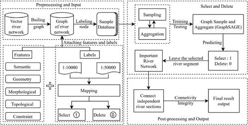
Step 1: River modelling. In the field of mapping, natural rivers are generally stored in vector form; however, the data requirements of GNNs require the conversion of the vector structure into a graph structure. The original river segments are abstracted as graph nodes based on dual graphs, and the node relationships are abstracted as edges based on the overlap of the first and last points of the river segments, with the graph structure used to represent the topological relationships of the river network data.

Step 2: Feature extraction and sample database construction. A supervised learning approach can be used to generalise a 1:10,000 river network map to 1:50,000. Using the identical entity matching method, selection markers are obtained by comparing river network data of the same area at different scales. Descriptive features of each graph node are extracted from semantic, geometric, morphological, and topological relationships as well as constraint conditions of each river segment as a basis for model training. The node features and generalisation markers from the sample library are converted into a data format that deep learning can recognise and process for training the GNN.

Step 3: Feature sampling and aggregation. The real-world river network has a complex structure and a large number of nodes, and the dual graph also has a variety of topological relationships. The sampling method is used to obtain the nodes associated with the target nodes in the dual graph of river segment data, and by aggregating feature vectors of neighbouring nodes, local information is transferred to the global level and richer and more abstract feature information is extracted from it.

Step 4: Selection model construction. A subset of node labels can be used to construct and train a GraphSAGE model, which is used to classify the nodes to determine whether the river segment is selected or not.

Step 5: River network test data selection. The GraphSAGE model is used to classify the river segments to be selected, and the selection of river network test data is achieved based on calculated probabilities. Finally, the connectivity and integrity of the river network is ensured by connecting the separate river segments and outputting the selected river network.

2.1. Modelling a road network as a graph

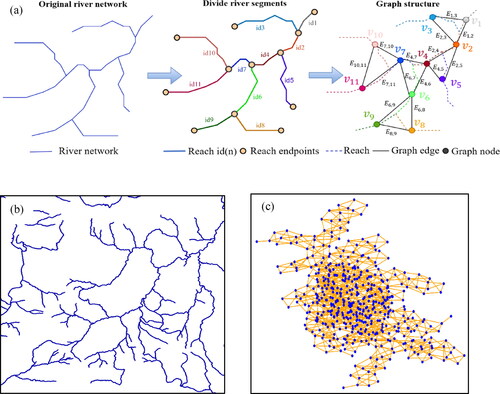
In the original vector map, river intersections are graph nodes and each river segment is an individual edge of the graph; however, in a dual graph of river network data, each river segment is regarded as a graph node and the connections between segments are regarded as edges. Compared to the original vector diagram, the dual graph provides a more intuitive understanding of the structure and connectivity of the river network and represents the nature of river segments and their topological relationships; therefore, this paper uses dual graphs to model river network data as a complete structure.

A river network dual graph is a network model that uses graph theory to describe a river network, and it can be defined as $G=(V,E,A),$ where the graph nodes are the midpoints of each river segment, denoted as $V=\{v_1, v_2,\dots ,v_n\};$ the connectivity between river segments is the edge connecting the graph nodes, denoted as $E=\left\{v_i{v}_j\right|v_i,v_j\in V\};$ and the adjacency matrix of the river network dual graph is constructed based on the relationships between the nodes $A\in R^{i*i}.$ The rows and columns of the matrix are the nodes of the dual graph respectively, and $i$ 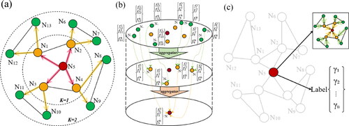denotes the number of nodes of the dual graph. An intersection point of two nodes with a topological relationship in the matrix has a value of 1, and the intersection point of nodes without a topological relationship has a value of 0. Figure 2 illustrates the process of building a river network dual graph, wherein (a) is the abstract building process of a river network dual graph, (b) is the actual river network, and (c) is the dual graph based on the actual river network. Rivers flow in a certain direction; however, when using a GNN for node classification, only inter-node relationships are considered while inter-directional relationships are not. Therefore, the river dual graph is a non-directional graph in this study. Dual graphs use edges to represent the connectivity of the original river network, describe the connection relationships between river segments, and calculate the degree of connectivity of the network using complex network methods, which improves the descriptive scope of graph structure data and achieves quantitative representation of topological relationships.

Figure 2. Graph modelling of a river network. (a) River network abstract dual graph representation; (b) primal river network; and (c) river network dual graph.

2.2. Extracting features and establishing a sample database

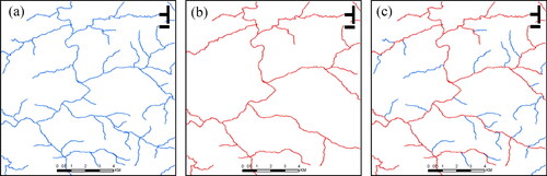
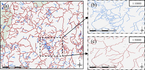
A wealth of expert knowledge is available in map results. The 1:10,000 and 1:50,000 river network data are pre-processed separately, buffers are constructed for different scales of river network data based on expert experience, and overlapping areas of the 1:10,000 and 1:50,000 river network buffers are calculated, with identical entity matching conducted. Based on existing research experience and experimental results, an area overlap threshold of 85% is set. If the overlap area of the river segment between the two scales of the size map exceeds 85%, then the river segment is selected, whereas if it is below 85%, then the matching fails and the river segment is deleted. In Figure 3, panels (a) and (b) are parts of the 1:10,000 and 1:50,000 scale river network, respectively, and panel (c) is the result of identical entity matching. Based on the above criteria, the red part should be retained and selected while the blue part should be deleted. By comparing river network data from the same area at different scales, the selection labels are automatically obtained.

Figure 3. Example of a river network matching result. (a) 1:10,000 scale river network data; (b) 1:50,000 scale river network data; and (c) matching result.

River network data features are an important basis for training deep learning models, and they directly influence the final selection of generalisation results. Each node in the graph structure carries a set of descriptive features to represent graph functions. Based on water system mapping research (Shao et al. 2004; Ai et al. 2007; Wu et al. 2007), each node is considered in terms of its attributes, geometry, morphology, relational structure, and scale constraints. Semantic features include river segment grade $O;$ geometric features include river segment length $L;$ and morphological features include river segment curvature $C=L_r/L_s,$ where $L_r$ is the actual length of the river segment and $L_s$ is the straight length of the river segment. In addition, topological features include the number of adjacent nodes $N\_n$ and the number of adjacent lakes $N\_l,$ with the number of adjacent nodes indicating the number of nodes in the graph structure that have a topological relationship with the node and the number of adjacent lakes establishing buffers at different scales according to the river segment grade and determining the total number of lakes within each river segment buffer. River network data at a scale of 1:25,000 are used as a constraint to reflect changes in the location, form, and size of the same geographical phenomena in multi-scale maps and improve the consistency and continuity of the map. The extracted characteristics and their meanings are shown in Table 1 below:

Table 1. Graph node characteristics.

Feature item		Description
Semantic feature	River order	Reflects importance: the higher the grade, the more important the river segment.
Geometric feature	River segment length	Reflects influence: the longer the river segment, the greater the scope of influence.
Morphological feature	River curvature	Reflects the velocity of the river: the greater the curvature of the river and the longer the length, the lower the velocity (because the water is spread over a larger area, the river flows less).
Topological features	Number of adjacent nodes	Reflects the upstream and downstream connections of the river segment: the more adjacent nodes in the graph structure, the more connected the river segment.
	Number of adjacent lakes	Reflects the developed hydrological system of the basin: the greater number of lakes, the more developed the hydrological system around the basin, which provides more water resources.
Binding feature	1:25,000 river network	Reflects the constraints of the network: a 1:25,000 scale river network of the same area is used to constrain and ensure the spatial consistency of the geographical elements.

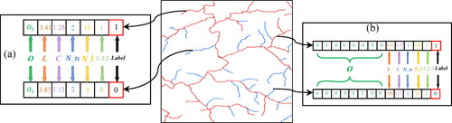
Node feature and matching labels are combined to obtain the river network selection sample library (Figure 4a). The computational model GraphSAGE can only manage numerical data. Semantic features tend to cause long training times for neural networks and failure of the model to converge, which is why a quantitative representation of river network features is required. The semantic features are discrete and disordered; therefore, the one-hot encoding technique is used to map the semantic features to numerical features and the eight ranked river segments are encoded using 8-bit memory, with only one independent register bit valid at any given moment in the encoding. Then, the ranked features of the river segments are expressed quantitatively in the GraphSAGE model. For numerical data, the Max-Min standardisation method is used to map the values of the data to a range of [0,1], as shown in Figure 4b, which reveals the encoded features.

Figure 4. River network selection sample coding. (a) Sample initial features; and (b) sample encoded features.

2.3. Sample and aggregate node features

GraphSAGE is a GNN model based on neighbour sampling that solves the problem of node classification and embedding in large-scale graphs. Instead of trying to learn the embedding of all nodes on a graph, the model learns to produce a map that generates embeddings for each node. The GraphSAGE framework contains two important operations: sampling and aggregation. The sampling method uses neighbour sampling, i.e. a few nodes are selected as first-order neighbours of the original node, after which it continues to select nodes among the neighbours of the newly sampled nodes as second-order nodes of the original node, and so on. Assuming that the number of layers to be sampled is $K$ and the number of neighbours sampled in each layer is $L_k,$ given a small set of nodes $\beta$ to sample, the first-order neighbours of $\beta$ are sampled to obtain ${\beta }_1$ and then the first-order neighbours of ${\beta }_1$ are sampled to obtain the second-order neighbours ${\beta }_2$ of the initial set of nodes, which continues for $K$ iterations to obtain the relevant subgraph of the initial small set of nodes.

Neighbour sampling is followed by neighbour aggregation. The standard neighbour aggregation functions are mean, max, and sum aggregation. Mean aggregation averages the features of neighbouring nodes to represent the feature of the current node, and it tends to learn the distribution. Max aggregation takes the maximum value of the features of neighbouring nodes to represent the feature of the current node, and it tends to ignore duplicate values. Sum aggregation adds the features of neighbouring nodes to represent the feature of the current node, and it can retain complete information of neighbouring nodes. The original structure of the river network is close to that of a tree, and sparse and regular connections occur between the nodes in the graph structure. Max aggregation is used to retain the most important features of neighbouring nodes to retain the influence of the surrounding important river segments, which better captures the important features of the nodes while reducing the differences in the features of neighbouring nodes.

Full neighbourhood sampling and aggregation of $K=2$ is performed for target node $N_5.$ In Figure 5a, nodes with a direct association, i.e. $N_1, N_2, N_3, \mathit{and} N_4,$ are sampled from $N_5$ in the $K=1$ layer, and then the neighbourhood nodes $N_6, N_7, N_8,$ $N_9, N_{10}, N_{11}, N_{12},$ and $N_{13}$ in the $K=2$ layer are obtained based on the first layer nodes. After the sampling of neighbouring nodes is completed, the features of neighbouring nodes need to be aggregated to the target node based on certain rules. As shown in Figure 5b, the aggregation direction is opposite the sampling direction, and the classification of graph nodes is completed by extracting river segment information with the help of information transmission (Figure 5c). Information transmission first combines the features of the edge and features of the nodes connected to the edge to obtain the information function. The information functions on the edges connected to the target node are then aggregated and finally combined with the existing node features of the target node, and it is classified. The information transmission equation is as follows: (1) $$m_q^k=\mathrm{\Phi }\left(f_p^{k+1},\mathrm{ }{f}_q^k\right),(p,q\in V)$$(1) (2) $$f_q^{k-1}=\psi (f_q^k,\rho \{m_q^k\left\}\right)$$(2) where $f_p^{k+1}$ and $f_q^k$ are the node features of nodes $p$ and $q,$ respectively; $m_q^k$ is the information between the neighbouring node $p$ and the target node $q;$ $\mathrm{\Phi }$ is the information function that combines the features of the two nodes to generate information; $\rho$ is the aggregation function that aggregates all the information; and $\psi$ is the renewal function that combines the aggregated information with the node’s own features to update the node features. Sampling and aggregating graph nodes consider both neighbouring river segment attribute features and connection relationships between segments, and a GraphSAGE-based river network feature aggregation model is established, thus enabling the updating and selection of river segment neighbourhood information based on the GNN.

Figure 5. River network neighbour sampling and aggregation. (a) Sample neighbourhood; (b) aggregate feature information from neighbours; and (c) categorisation using aggregated information.

2.4. Construction of a graph neural network classification model

2.4.1. Graph neural network structure

This paper uses PyTorch Geometric library in python to implement the classification model, and the river segment classification model based on the GraphSAGE framework consists of three main parts: input layer, hidden layer, and output layer. Figure 6 represents the input of a graph structure and the classification of the graph structure node labels by embedding the graph in a high-dimensional vector through convolution and linear classification. The hidden layer of the model includes the three convolutional layers of SAGEConv and the Rectified Linear Unit (ReLU) activation function, SAGEConv is a convolution method of adaptive filtering, the mathematical equation is as follows: (3) $$h_{\mathcal{N}\left(\mathit{dst}\right)}^l=\mathit{aggregate}\left(\right\{h_{\mathit{src}}^{l+1},{\forall }_{\mathit{src}}\in \mathcal{N}\left(\mathit{dst}\right)\left\}\right)$$(3) (4) $$h_{\mathit{dst}}^l=\sigma (W·\mathit{concat}(h_{\mathit{dst}}^{l+1},h_{\mathcal{N}\left(\mathit{dst}\right)}^l)+b)$$(4) (5) $$h_{\mathit{dst}}^l=\mathit{norm}\left(h_{\mathit{dst}}^l\right)$$(5) where $h_{\mathit{dst}}^l$ is the target node feature and $h_{\mathit{dst}}^{l+1}$ is the neighbouring node feature. The ReLU activation function is a widely used non-linear activation function applied to the output of a neuron with characteristics such as sparsity and resistance to the vanishing gradient problem. The mathematical equation is as follows: (6) $$f\left(x\right)=\max (0,x)(x<0,x=0;x\ge 0,x=x)$$(6)

Figure 6. Graph classification model based on GraphSAGE, which contains two convolutional layers (SAGEConv): a fully connected layer (linear) and a normalised exponential layer (Softmax).

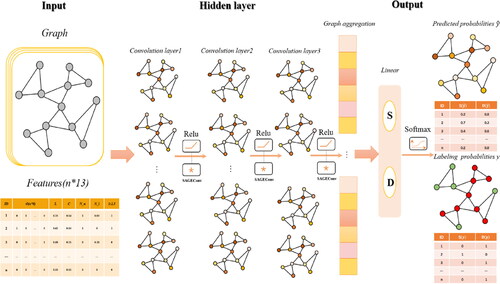
The output layer of the model is a fully connected layer that receives the output of the second hidden layer as input and returns the node classification probability distribution as output, which is mapped to an output vector of size ‘out channels’ by a linear classification layer ‘Linear’. The mathematical equation for linear classification is as follows: (7) $$f\left(x,W\right)=Wx+b$$(7) where $f\left(x,W\right)$ is the output vector, $x$ is the input vector, $W$ is the parameter or weight matrix, and $b$ is the bias vector. During classification, the activation function Softmax is used to normalise the output of the neural network to a probability distribution, where each output node represents a category and the output value of each node represents the probability of that category. The mathematical equation is as follows: (8) $$f\left(x_i\right)=\frac{e^{x_i}}{\sum _i{e}^{x_i}}$$(8) where $f\left(x_i\right)$ denotes the node output feature value and the denominator denotes the sum of the river segment selection and deletion values. The sum of the output of the Softmax function is 1, which can be interpreted as the probability of each category. The process is primarily a graph classification process, where the high-dimensional vectors obtained by the classifier are classified to complete the river segment selection task.

2.4.2. Model optimisation

In GNN learning, model optimisation makes the model fit the data better and improves the accuracy and generalisation of the model. In classification problems, model performance is often measured using the cross-entropy function, which is calculated based on the output of the Softmax function and represents a loss function used to measure the difference between the predicted and true values of a model. This function is calculated as follows: (9) $$L=-\left[y\log \hspace{0.17em}\widehat{y}+\left(1-y\right)\log \hspace{0.17em}\left(1-\widehat{y}\right)\right],\left(\widehat{y}ϵ\right(0,1\left)\right)$$(9) where y is the true label and $\widehat{y}$ is the predicted probability value, which characterises the difference between the true sample label and the predicted probability. The cross-entropy loss function can effectively solve problems such as vanishing and exploding gradients and improve the stability of the model parameter updates. In a binary classification problem, the smaller the cross-entropy function, the smaller the error value of the probability distribution between the predicted and actual values, and the higher the classification accuracy.

Adaptive momentum (Adam) is a stochastic optimisation method that combines the advantages of gradient descent and moment methods to iteratively update neural network weights based on training data. The mathematical formula is as follows: (10) $$m_t=\mathit{\mu }\mathrm{*}{m}_{t-1}+\left(1-\mathit{\mu }\right)\mathrm{*}{g}_t$$(10) (11) $$n_t=v\mathrm{*}{n}_{t-1}+\left(1-v\right)\mathrm{*}{g}_t^2$$(11) (12) $${\widehat{m}}_t=\frac{m_t}{1-{\mu }^t}$$(12) (13) $${\widehat{n}}_t=\frac{n_t}{1-v^t}$$(13) (14) $$\mathrm{\Delta }{\mathit{\theta }}_t=-\frac{{\widehat{m}}_t}{\sqrt{{\widehat{n}}_t}+\epsilon }\mathrm{*}\eta$$(14) where $m_t$ and ${\widehat{m}}_t$ are the gradient first-order moment estimate and correction, respectively, $n_t$ and ${\widehat{n}}_t$ are the gradient second-order moment estimate and correction, respectively, and $\mathrm{\Delta }{\theta }_t$ is the dynamic constraint on the learning rate. The gradient first-order moment estimation of the Adam algorithm has inertia-maintaining properties that allow for smooth stable transitions at each update, and the second-order moment estimation has an environmental awareness function that generates adaptive learning rates for different parameters, resulting in faster convergence to the optimal solution.

3. Experimental results and analysis

3.1. Experimental data

The experimental study area is part of the Min River system in the Yangtze River Basin in China. In addition, 1:10,000 water system data were used as the experimental data, including a total 2723 river segment. The proportion of training, verification and testing data was 8:1:1, and 1:50,000 data were used as the reference results (Figure 7). First, disordered lines with no connection relationships within the experimental area were deleted, and then the centre lines of the double-lined areas at the large scale were extracted as the objects of study. Topological checks were conducted according to rules such as no hanging points and no false nodes, and each river in the overall regional water system was divided into river segments from the intersection points. Finally, in accordance with section 2.2, a sample library of river segment-based dual graphs and map nodes was constructed. The example graph structure contained a total of 2723 nodes and 8262 edges, which were used as the input layer for training and testing to complete graph node classification and river network data selection.

Figure 7. Experimental data: (a) 1:10,000 and 1:50,000 overlays; (b) 1:10,000 partial area; and (c) 1:50,000 partial area.

3.2. Classification performance of river segments

3.2.1. Comparison of different learning models

The experiment in this paper used a five-layer GraphSAGE model with three convolutional layers, one linear classification layer, and one normalised exponential layer. The model included 13 feature dimensions in the input layer, 128 embedded vector dimensions, and 128 input and 2 output dimensions in the fully connected layer, and the activation functions were all ReLU functions. The experimental results revealed that the loss value dropped to 0.02 at the end of training and the accuracy of the validation set was 90%. The model converged well after 400 iterations.

In the experiment, the classification models were compared with three other graph convolutional neural network models, namely, the Graphics Core Next (GCN), Graph Attention Network (GAT), and Graph Intention Network (GIN) models, all of which were trained using the Adam algorithm. Each convolutional layer contained 128 cores and had a learning rate of 0.005 and a maximum number of iterations of 500. The GAT head was set to 4. Figure 8 shows the changes in loss values and accuracy curves as the number of iterations increased.

Figure 8. Loss value and accuracy curves of neural network models in different graphs. (a) Loss value change curve of different models; and (b) validation dataset accuracy curve of different models.

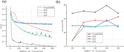
The performance of the four models for the same dataset revealed that the GraphSAGE model had a smooth and stable decrease in loss (Figure 8a) without significant jumps or oscillations, thus indicating that the model could well fit the dataset. The decreasing trend levelled off in the later stages, and the final loss value was <0.1, indicating that the model had converged and the training results were good. Figure 8b shows the validation dataset accuracy at every 100 iterations. The accuracy of the models initially increased as the number of iterations increased and tended to stabilise thereafter, indicating that the models converged. The GraphSAGE model had the highest accuracy for the validation set at epoch = 400. In summary, the GraphSAGE model has good generalisation capabilities for the classification of graph nodes in this dataset, is effective at classifying node sensitivity, and can effectively select river segments.

3.2.2. Model parameter sensitivity analysis

In the experiment, the influence of model hyperparameters on the accuracy of the model was analysed. These hyperparameters included the number of node features, activation function, loss function, aggregation function, optimiser, and model depth.

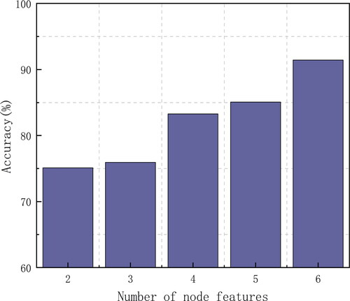
The effect of different numbers of node attributes on the accuracy of the model was analysed when other hyperparameters, such as model depth and shape embedding vector, are certain. As a unique non-Euclidean spatial data structure, the spatial characteristics of graph data and attribute characteristics of graph nodes have an important impact on graph structure data. The objectivity of node feature extraction was analysed and the model was trained using different numbers of node features to investigate the classification performance of the model. As shown in Figure 9, at epoch = 400, the accuracy of the model after training was approximately 75% when two node features and only the number of neighbouring nodes and lakes topological features were included. After adding geometric (length of river segment), semantic (grade of river segment), and morphological (curvature of river segment) features, the accuracy was improved to over 85% and the number of node features was increased to five. Finally, after adding the constraint feature, the accuracy significantly improved to 90%, which indicated that the selection of individual features and constraint features among node features played a significant role in promoting the model classification.

Figure 9. Influence of the number of node features on accuracy.

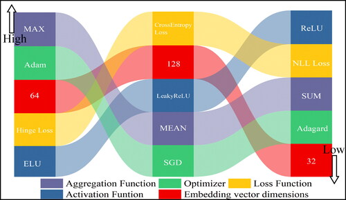
The effect of model hyperparameters on model performance, including the shape embedding vector dimension, activation function, loss function, aggregation function, and optimiser, was investigated for a given model when the learning rate, number of node features, and model depth conditions were constant. Under certain conditions, the higher the dimensionality of the shape embedding vector, the higher the classification accuracy of the model; therefore, a value of 128 was selected as the number of dimensions for the shape embedding vector. With an embedding vector dimension of 128, ReLU, ELU, and LeakyReLU were chosen as the activation functions; CrossEntropy Loss, NLL Loss, and Hinge Loss were chosen as the loss functions; max, mean, and sum were chosen as the aggregation function; and Adam, SGD, and Adagard were chosen as the optimizers for comparison. The experimental results revealed that the three different activation and loss functions yielded similar accuracy results, with ReLU and CrossEntropy Loss yielding the best results. The different optimizers and aggregation methods varied significantly, with the max aggregation and Adam optimiser yielding significantly higher accuracy than the other parameters (Figure 10).

Figure 10. Influence of different hyperparameters on the accuracy of the model.

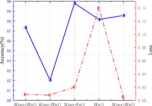
The hyperparameters of the optimal model were experimentally determined to further investigate the effect of model depth on model classification performance. The effect of model depth on model performance was investigated with fixed hyperparameters and node features, an embedding vector dimension of 128, a learning rate of 0.005, and a few iterations of 400. The classification accuracy and loss of the model were used as indicators to evaluate performance, and four different depths were used for comparison with the original model, namely, 3Conv + 2Full, 4Conv + 2Full, 5Conv + 2Full, and 2Full. The results are shown in Figure 11. A comparison of the models with different depths and structures showed that all models except for the fully connected neural network model 2Full had a loss value below 0.02. The model 3Conv + Full in this study had a maximum classification accuracy of 90%, and as the depth and weight dimensions of the model increased, the model structure became more complex, which caused overfitting and thus weakened the generalisation ability of the model. Model 3Conv + Full had the highest accuracy and best performance, indicating that the model structure was better able to learn the semantic, geometric, morphological, and topological constraint relationships of river segments and other features to improve the model classification accuracy.

Figure 11. Accuracy and loss values of different depth models.

3.3. Classification accuracy analysis

To measure the suitability of a classification model for river segment selection, predictions were made for each sample in each test set and an evaluation score was calculated based on the results of the model’s predicted classifications. The confusion matrix, accuracy, precision, recall F1_Score, and AUC area are commonly used as model evaluation metrics. The confusion matrix consists of TN, FN, TP, and FP; accuracy (Acc) measures the proportion of correct classifications; precision (Pre) refers to the proportion of data predicted to be positive samples that are predicted correctly; recall (Rec) is the probability that actual positive samples will be predicted as positive for the original samples; F1_Score considers both precision and recall and allows both to segment their highest level while striking a balance; and AUC area is the size of the area under the ROC curve based on the true positive rate and false positive rate. AUC is a performance indicator that measures the superiority of the model, and a larger AUC corresponds to a better current classification effect, which can eliminate the effect of sample category imbalance on the index result. Acc, Pre, Rec, and F1_Score are calculated as follows: (15) $$\mathit{Acc}=\mathrm{ }\frac{TP+TN}{TP+TN+FP+FN}$$(15) (16) $$\mathit{Pre}=\frac{TP}{TP+FP}$$(16) (17) $$c=\mathrm{ }\frac{TP}{TP+FN}$$(17) (18) $$F1\_\mathit{Score}=\frac{2Pre\cdot \mathit{Rec}}{\mathit{Pre}+\mathit{Rec}}$$(18) $Re$ where P denotes positive sample predictions; N denotes negative sample predictions; T denotes correct predictions; F denotes a false sample prediction; TP and TN denote the number of samples selected and deleted for correct classification; FP and FN denote the number of samples selected and deleted for incorrectly classification.

The statistics of the model’s classification effectiveness indicators are shown in Table 2. The model achieved good test results with a good fit, and the Acc, Pre, Rec, and F1_Score were all above 95%. The ROC curve had a high TPR and low FPR, and the AUC was 0.94, indicating that the model had high sensitivity and a low false positive rate, which is equivalent to an excellent classification performance, good learning ability, and excellent generalisation ability.

Table 2. Test set classification result statistics.

Evaluation index	TP	FP	FN	TN
	218	5	0	50
	Acc (%)	Pre (%)	Rec (%)	F1_Score (%)
	98.17	98.63	99.08	98.86

3.4 Contrast experiment

To verify the difference between the model and other classification methods, the support vector machine (SVM), random forest (RF) and naïve Bayes (NB) classification methods were used for comparison. In the algorithm comparison test, model classification was implemented with the help of the Scikit-learn (Sklearn) library in Python and the algorithm parameter values were optimized to effectively improve model performance.

As shown in Figure 12, in the SVM algorithm, the penalty coefficient C = 1 was chosen to control the complexity of the model and the kernel function coefficient gamma = 1 was used to control the distribution of the samples after being mapped to a high-dimensional space. In the RF algorithm, model performance was mainly affected by the number of decision trees, which affected the accuracy and running speed of the model. Usually, a higher number of decision trees in the RF corresponds to a higher the accuracy of the model; however, such model configurations can also increase the computation time and memory usage of the model. The experiment used the sampling method with replacement and chose a value of 200 as the appropriate number of decision trees. In the NB algorithm, the prior probability of the first category was set in the prior parameter, and the classification result for priors= [0.1,0.9] was selected.

Figure 12. Accuracy of the compared methods.

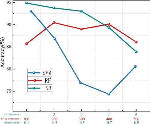
The results obtained for the comparison experiments were tested on the test set. The classification results for GraphSAGE, SVM, RF, and NB are shown in Table 3. In the field of machine learning, SVM, RF, and NB are all commonly used in classification tasks; however, the graph CNN delivered higher classification results than all three. This is because the river network can extract and retain the spatial geometric features of river segments and the relationships and connections between river segments to the greatest extent after the construction of the river segment graph structure. During graph convolution operations, the attributes of river segments are expanded by dimensionality to achieve higher-resolution attribute representation. In addition, the attributes between river segments are aggregated and passed on to achieve the combination and extraction of shape features of adjacent river segments. Multi-layer graph convolution extracts river segment features at different levels through serial connections, thereby increasing the depth of the network, allowing more abstract features to be extracted layer by layer, ensuring the aggregation of higher-order long-range shape features, accounting for the topology between river segments during the convolution process, and achieving an encoded representation of graph information through multiple levels of local features, thus providing a significant gain effect for the final classification.

Table 3. Comparison of classification accuracy among similar algorithms.

Index	GraphSAGE	SVM	RF	NB
Accuracy (%)	98.17	93.04	90.47	94.87

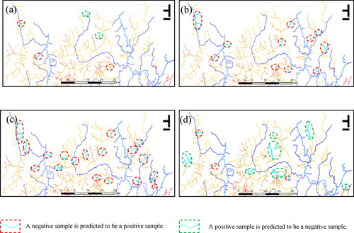
The prediction results are shown in Figure 13. Panels a–d show the prediction errors for river segments by GraphSAGE, NB, RF, and SVM. GraphSAGE had the lowest number of prediction errors, and RF had the highest number of prediction errors at over 20. The areas contained in red dotted ellipses are the negative samples misclassified as positive, and the areas contained in green dotted ellipses are positive samples misclassified as negative, i.e. the former are segments that should have been deleted but were retained and the latter are segments that should have been retained but were deleted. In this test area, the number of positive samples was greater than the number of negative samples, and all misclassified segments by the NB and RF algorithms should have been deleted but were retained. Therefore, a trends of misclassifying negative samples as positive samples was observed, resulting in a higher false positive rate and a lower accuracy. Within the region, from the perspective of semantic features, river segments with higher grades usually play a more important role and status in the river network structure. The river grades deleted by this method mainly focus on grades 3 and 4, while NB and RF deleted several grade 2 segments, indicating that the importance of river segment grades is well taken into account by this method. From the perspective of geometric features, a longer river segment usually has more complex, extensive and abundant resources and functions than a shorter one. Compared with the methods in this paper, RF and SVM delete more long river segments, and the influence of the importance of river segments is poorly considered. From the perspective of topological relationship, in both RF and SVM, samples of the river segment with two connections were misclassified, that is, the intermediate river segment with connection condition at both ends is deleted, which is contrary to the principle of river connectivity. Therefore, from the perspective of semantic, geometric and topological features, the method proposed in this study was more accurate because it considers the overall number of misclassifications, the class and length of the river segment, and the maintenance of the river network structure.

Figure 13. Incorrect results predicted by different classification methods. (a) Misclassified river segment by GraphSAGE. (b) Misclassified river segment by NB. (c) Misclassified river segment by RF. (d) Misclassified river segment by SVM.

4. Discussion

The experimental results show that the classification accuracy of river segments based on the graph structure in this paper was better than that of traditional models.

First, this paper introduced a graph CNN to river network selection for the first time, thereby enriching the methods of river network selection and achieving better classification results. Moreover, the selected river segments were not cut off in the middle of connections but maintained a complete river, thereby ensuring the connectivity and integrity of the river.

Second, in terms of feature selection, river segments were used as the basic unit, their features, spatial relationships, and constraints were considered, and the connectivity between river segments was constrained by using the connection characteristics at both ends of river segments, which guarantees the integrity of the river network map structure and ensures the self-similarity and integrity of the river network before and after selection. Moreover, as the number of features increased, the correct classification rate of the model increased.

The GraphSAGE model was more efficient at processing large-scale graph data and was able to capture relationships and influences between river segments by obtaining more comprehensive node characteristics through sampling and aggregation based on neighbourhood information. When applied to different morphological river network data from different regions, it can be flexibly adapted and customized using different sampling strategies, aggregation functions, and loss functions to learn a generic representation of nodes in the graph structure.

Finally, river network data represent typical graph structure data. The graph CNN efficiently learned and classified features in the graph structure data and extracted advanced and complex sample features from simple geometric and topological structures using embedding vectors, which not only achieves better results in river network morphology recognition but also improves the accuracy and efficiency of river network selection. Therefore, the proposed method is suitable for river network generalisation applications.

5. Conclusions

In response to the lack of research on river network selection using GNNs, this paper proposed a method of river network selection based on the GNN GraphSAGE. The method considers river segments in a river network as the basic unit, extracts semantic, geometric, morphological, topological, and constraint features of river segments as graph node attributes, and expresses topological relationships between river segments in a graph structure. The graph with labels and node attributes is used as the input data of the classification model with the support of case studies. Through supervised training, sampling and aggregation methods are used to obtain more abundant and abstract feature information, and the graph CNN model GraphSAGE is used to classify river segments for selection and deletion in large-scale river network maps. The GNN method enriches the methods of generalizing river network map data by extending the individual characteristics of river segments to the complex relationships between nodes in the graph structure. This characteristic enables deeper identification of relationships within the river network and improves the rate of correct river network selection. The method was tested on the 1:10,000 scale Minjiang River system. The five-layer GraphSAGE classification model, with a 1:50,000 scale map as the reference for the selection of a 1:10,000 scale river network, achieved over 95% accuracy. Moreover, its accuracy was 7.35%–5.31% higher than that of the other GNN methods and 7.7%–3.3% higher than that of traditional machine learning methods.

In this paper, only a few constraints and topological features were extracted. In subsequent research, more information including topological features, such as river spacing, symmetry between left and right tributaries, and river branching, as well as constraint features, such as the importance of the surrounding road network, residential areas, and buildings should be assessed. Training tests could also be conducted on larger- and smaller-scale river network datasets and at different scales to verify the generality of the model.

Author contributors

Di Wang composed the original idea of this study, implemented the code, contributed to writing, and finished the first draft. Haizhong Qian supervised the research and edited and reviewed the manuscript.

Data availability statement

The data and codes that support the findings of this study are available in Figshare at https://doi.org/10.6084/m9.figshare.22793993.v1

Disclosure statement

No potential conflict of interest was reported by the authors.

Additional information

Funding

This work was supported by the National Natural Science Foundation of China [42271463] and Natural Science Foundation for Distinguished Young Scholars of Henan Province [212300410014].

References

- Abdel-Hamid O, Mohamed A, Jiang H, Deng L, Penn G, Yu D. 2014. Convolutional neural networks for speech recognition. IEEE/ACM Trans Audio Speech Lang Process. 22(10):1533–1545. doi: 10.1109/TASLP.2014.2339736.
- Ai T, Liu Y, Huang Y. 2007. The Hierarchical watered partitioning and generalisation of river network. J Sur Map. 36(02):231–236. +243.
- Ai T. 2021. Some thoughts on deep learning enabling cartography. Acta Geod Cartogr Sin. 50(09):1170–1182.
- An J, Guo L, Liu W, Fu Z, Ren P, Liu X, Li T. 2021. IGAGCN: information geometry and attention-based spatiotemporal graph convolutional networks for traffic flow prediction. Neural Netw. 143:355–367. doi: 10.1016/j.neunet.2021.05.035.
- Anderson-Tarver C, Buttenfield BP, Stanislawski LV, Koontz JM. 2011. Automated delineation of stream centerlines for the USGS National Hydrography Dataset. Adv Cartogr GISci. 1:409–423.
- Buttenfield BP, Samaranayake VA. 2010 Sept 12–13. Generalization of hydrographic features and automated metric assessment through bootstrapping. In: 13th Workshop of the International Cartographic Association commission on Generalisation and Multiple Representation, Zurich, Switzerland.
- Buttenfield BP, Stanislawski LV, Anderson-Tarver C, Gleason MJ. 2013. Automatic enrichment of stream networks with primary paths for use in the United States national atlas. In: Proceedings, International Cartographic Conference (ICC2014), Dresden Germany.
- Chen C, He W, Zhou H, Xue Y, Zhu M. 2020. A comparative study among machine learning and numerical models for simulating groundwater dynamics in the Heihe River Basin, northwestern China. Sci Rep. 10(1):3904. doi: 10.1038/s41598-020-60698-9.
- Du J, Wu F, Zhu L, Liu C, Wang A. 2022. An ensemble learning simplification approach based on multiple machine-learning algorithms with the fusion using of raster and vector data and a use case of coastline simplification. Acta Geod Cartogr Sin. 51(03):373–387.
- Duan P, Qian H, He H, Liu C, Xie L. 2019. A lake selection method based on dynamic multi-scale clustering. Geom Inf Sci Wuhan Univ. 44(10):1567–1574.
- Duan P, Qian H, He H, Xie L, Luo D. 2019. Naive Bayes-based automatic classification method of tree-like river network supported by case. Acta Geod Cartogr Sin. 48(08):975–984.
- Gong J, Ji S. 2018. Photogrammetry and deep learning. J Geod GI Sci. 1(1):1–15.
- Guo X, Qian H, Wang X, Liu J, Ren Y, Zhao Y, Chen G. 2022. Ontology knowledge reasoning method for multi-source intelligent road selection. Acta Geod Cartogr Sin. 51(02):279–289.
- Hamilton W, Ying Z, Leskovec J. 2017. Inductive representation learning on large graphs. Adv Neural Inf Proc Sys. 30:1025–1035.
- Han M, Su Z, Na X. 2023. Predict water quality using an improved deep learning method based on spatiotemporal feature correlated: a case study of the Tanghe Reservoir in China. Stoch Environ Res Risk Assess. 37(7):2563–2575. doi: 10.1007/s00477-023-02405-4.
- Jiang L, Qi Q, Zhang A. 2015. River classification and river network structuration in river auto-selection. Geom Inf Sci Wuhan Univ. 40(06):841–846.
- Krizhevsky A, Sutskever I, Hinton G. 2017. Imagenet classification with deep convolutional neural networks. Commun ACM. 60(6):84–90. doi: 10.1145/3065386.
- LeCun Y, Bengio Y, Hinton G. 2015. Deep learning. Natur. 521(7553):436–444. doi: 10.1038/nature14539.
- Li C, Wu W, Yin Y. 2018. Hierarchical elimination selection method of dendritic river network generalization. PLoS One. 13(12):e0208101. doi: 10.1371/journal.pone.0208101.
- Li C, Yin Y, Wu W, Wu P. 2018. Method of tree-like river networks hierarchical relation establishing and generalization considering stroke properties. J Sur Map. 47(4):537–546.
- Liu C, Zhai R, Qian H, Gong X, Wang A, Wu F. 2023. Identification of drainage patterns using a graph convolutional neural network. Trans GIS. 27(3):752–776. doi: 10.1111/tgis.13041.
- Long S, Wu T, Sun G, Feng D, Tong L, Xing M. 2020. Object detection research of SAR image using improved faster region-based convolutional neural network. J Geod GISci. 3(3):18–28.
- Long Y, Cao Y, Shen J, Li W, Zhou D. 2011. Cooperative generalization method of contour cluster and river network based on constrained D-TIN. Acta Geod Cartogr Sin. 40(03):379–385.
- Lu B, Gan X, Jin H, Fu L, Wang X, Zhang H. 2022. Make more connections: urban traffic flow forecasting with spatiotemporal adaptive gated graph convolution network. ACM Trans Intell Syst Technol. 13(2):1–25. doi: 10.1145/3488902.
- Ni Q, Cao X, Tan C, Wen P, Kang X. 2023. An improved graph convolutional network with feature and temporal attention for multivariate water quality prediction. Environ Sci Pollut Res Int. 30(5):11516–11529. doi: 10.1007/s11356-022-22719-0.
- Savino S. 2014. Generalization of braided streams. In: 17th ICA Workshop on Generalisation and Multiple Representation, Vienna, Austria.
- Sen A, Gokgoz T. 2015. An experimental approach for selection/elimination in stream network generalization using support vector machines. Geo Int. 30(3):311–329. doi: 10.1080/10106049.2014.937466.
- Shao L, He Z, Ai Z, Song X. 2004. Automatic generalization of a river network based on BP neural network. Geom Inf Sci Wuhan Univ. 29(06):555–557.
- Shi W, Sui H. 2022. An effective superpixel-based graph convolutional network for small waterbody extraction from remotely sensed imagery. Int J Appl Earth Obs Geoinf. 109:102777. doi: 10.1016/j.jag.2022.102777.
- Stoter J, Post M, van Altena V, Nijhuis R, Bruns B. 2014. Fully automated generalization of a 1: 50k map from 1: 10k data. Cartogr Geog Inf Sci. 41(1):1–13. doi: 10.1080/15230406.2013.824637.
- Sun A, Jiang P, Yang Z, Xie Y, Chen X. 2022. A graph neural network (GNN) approach to basin-scale river network learning: the role of physics-based connectivity and data fusion. Hydrol Earth Syst Sci. 26(19):5163–5184. doi: 10.5194/hess-26-5163-2022.
- Wang D, Qian H, Zhao Y. 2022. Review and prospect: management, multi-scale transformation and representation of geospatial data. GIScience. 24(12):2265–2281.
- Wang G, Wu M, Wei X, Song H. 2020. Water identification from high-resolution remote sensing images based on multidimensional densely connected convolutional neural networks. Remote Sens. 12(5):795. doi: 10.3390/rs12050795.
- Wang S, Zhang M, Miao H, Peng Z, Yu PS. 2022. Multivariate correlation-aware spatio-temporal graph convolutional networks for multi-scale traffic prediction. ACM Trans Intell Syst Technol. 13(3):1–22. doi: 10.1145/3469087.
- Wang W, Yan H, Lu X, He Y, Liu T, Li W, Li P, Xu F. 2023. Drainage pattern recognition method considering local basin shape based on graph neural network. Int J Digital Earth. 16(1):593–619. doi: 10.1080/17538947.2023.2172224.
- Wang W, Yan H, Lu X, Liu T, Wang Z. 2021. A review of automatic generalization research on map river networks. Geog GISci. 37(05):1–8.
- Wu B, Liang X, Zhang S, Xu R. 2022. Frontier advances and applications of graph neural networks. Chi J Comp. 45(01):35–68.
- Wu F, Du J, Qian H, Zhai R. 2022. Developments and reflections on intelligent map generalization. Geom Inf Sci Wuhan Univ. 47(10):1675–1687.
- Wu F, Tan X, Wang H, Zhai R. 2007. Study on automated canal selection. J Image Graphics. 12(06):1103–1109.
- Wu H, Ng M. 2022. Hypergraph convolution on nodes-hyperedges network for semi-supervised node classification. ACM Trans Knowl Discov Data. 16(4):1–19. doi: 10.1145/3494567.
- Xia T, Lin J, Li Y, Feng J, Hui P, Sun F, Guo D, Jin D. 2021. 3DGCN: 3-dimensional dynamic graph convolutional network for citywide crowd flow prediction. ACM Trans Knowl Discov Data. 15(6):1–21. doi: 10.1145/3451394.
- Xiao T, Ai T, Yu H, Yang M, Liu P. 2023. A point selection method in map generalization using graph convolutional network model. Cartogr Geogr Inf Sci. 50(3):1–21. doi: 10.1080/15230406.2023.2187886.
- Yang M, Jiang C, Yan X, Ai T, Cao M, Chen W. 2022. Detecting interchanges in road networks using a graph convolutional network approach. Int J Geogr Inf Sci. 36(6):1119–1139. doi: 10.1080/13658816.2021.2024195.
- Yu H, Ai T, Yang M, Huang L, Gao A. 2023. Automatic segmentation of parallel drainage patterns supported by a graph convolution neural network. Expert Syst Appl. 211:118639. doi: 10.1016/j.eswa.2022.118639.
- Yu H, Ai T, Yang M, Huang L, Yuan J. 2022. A recognition method for drainage patterns using a graph convolutional network. Int J Appl Earth Obs Geoinf. 107:102696. doi: 10.1016/j.jag.2022.102696.
- Yu Y, He K, Wu F, Xu J. 2022. A graph convolutional neural network approach for shape classification of faceted residential land. Acta Geod Cartogr Sin. 51(11):2390–2402.
- Zheng J, Gao Z, Ma J, Shen J, Zhang K. 2021. Deep graph convolutional networks for accurate automatic road network selection. Int J Geo-Inf. 10(11):768. doi: 10.3390/ijgi10110768.
- Zhou J, Cui G, Hu S, Zhang Z, Yang C, Liu Z, Wang L, Li C, Sun M. 2020. Graph neural networks: a review of methods and applications. AI Open. 1:57–81. doi: 10.1016/j.aiopen.2021.01.001.