Using the Google Earth Engine cloud-computing platform to assess the long-term spatial temporal dynamics of land use and land cover within the Letaba watershed, South Africa

Abstract

Population growth and environmental shifts have elevated the pressure on land use and cover (LULC), necessitating vital management and adaptive strategies to preserve the balance between ecosystem services and human well-being in watersheds. It's pivotal to understand the implications of human-induced shifts from natural to human-dominated surroundings This study utilized Google Earth Engine (GEE) to analyze 31 years of LULC changes in Letaba watershed. Using GEE's random forest, LULC classes were mapped with 93% to 99% accuracy across four timeframes (1990, 2000, 2010, and 2021). Trends revealed declining water bodies (-4%), bare surfaces (-2%), natural forest (-3%), and grassland (-3%), while shrublands, plantations, and built-up areas increased at annual rates of 41%, 24%, and 47% respectively. This transformation reflects population-driven shifts, necessitating adaptive strategies. Given the importance of plantations for income, embracing climate-smart agriculture could ensure long-term food and environmental security, thus addressing the evolving dynamics in Letaba watershed.

Keywords:

• Catchment health
• cloud computing
• ecosystem system
• environmental security
• land resources
• population growth

1. Introduction

Land resources form the most important source of livelihoods and pro key ecosystem goods and services globally. They play a vital role in supporting human needs, such as housing, food production, and settlement, as well as ecosystem services like climate regulation, soil formation, nutrient cycling, and supporting natural vegetation (Alemayehu et al. 2009; Amsalu et al. 2007; Mekuriaw 2017). However, the rapid growth of the population has led to increased pressure on land resources, resulting in changes in Land Use and Land Cover (LULC). Land use refers to how humans utilize and manage the land for various purposes. Land cover, on the other hand, refers to the physical and biological surface characteristics of the land (Jansen and Di Gregorio 2002; Mendoza et al. 2011). Such changes are the primary cause of global environmental modifications (Liping et al. 2018). For instance, Salazar et al. (2015) found that LULC changes impact land surface climate feedbacks, altering the exchange of heat, moisture, momentum, trace-gas flux, and albedo, which in turn affected local and regional climate. Additionally, Bufebo and Elias (2021) reported that LULC changes leads to soil and water quality degradation, loss of biodiversity, and reduced ability of watersheds to sustain natural resources and ecosystem services.

To effectively manage LULC, it is crucial to understand the processes driving their changes, the forces transforming natural habitats into human-dominated environments, and their consequences. This understanding will help in implementing appropriate LULC planning practices within watersheds, which play a vital role in managing soil and water resources worldwide (Grecchi et al. 2014; Kerr and Chung 2002). However, consistent monitoring has been lacking in many sub-Saharan African countries, especially in rural catchments.

Remote sensing technology continued to provide the spatial and temporal coverage, and is necessary for monitoring the environment, due wide observation range (Cui et al. 2022). Globally, numerous studies have been carried out on LULC change monitoring based on remote sensing. Shen et al. (2022) used time series Landsat to classify the LULC in Huangshui river Basin in China from 1987 to 2018 based on Random Forest (RF) and detected bidirectional spatio-temporal changes based on the distribution probabilities. Similarly, Zurqani et al. (2018), utilized Landsat 5 and 8 images to map land use changes of Savanna River basin in United State of America (USA) from 1999 to 2015 using on RF. Pan et al. (2022) classified LULC using Landsat 5 and 8 images in Australia and USA based on CART and RF. Furthermore, Leta et al. (2021) used Landsat to model and predict LULC in Upper Blue Nile Basin Ethiopia from 1990 to 2019 based Land change modeler and further predicted future LULC for 2035 and 2050. These studies confirm the effectiveness of remote sensing in extracting LULC changes.

Availability of satellite imagery data from platforms such as Landsat, Sentinel, MODIS, and other commercial satellites has greatly improved. These datasets provide consistent seasonal and long-term coverage, allowing for the analysis of LULC changes over time (Mashala et al. 2023). However, traditional methods of hardware and software are time consuming, as they require much time to perform image processing, mosaicking when working on a larger scale (Gorelick et al. 2017; Kumar and Mutanga 2018). This leads to massive challenges in remote sensing data download and low processing efficiency on large scale.

The emergence of remote sensing cloud computing, and cloud storage platform provide new technical for downloading and processing massive remote sensing data. Cloud-computing platform Google Earth Engine (GEE) is convenient for remote sensing data for desktops which enable high speed analysis using advanced processing techniques (Hoque et al. 2022; Sidhu et al. 2018). The cloud computing can integrate more than 200 remote sensing dataset and provide python and JavaScript to facilitate users to process data according to their own needs (Shafizadeh-Moghadam et al. 2021). GEE host advanced classification which enables one to run supervised learning algorithms across huge datasets (Lee et al. 2016; Cui et al. 2022). Algorithms that are found in GEE include Random Forest (RF), classification and regression tree (CART), support vector machine (SVM), Naive Bayes (NB) classifiers can accurately distinguish classes within a heterogeneous watershed.

However, most studies revealed the effectiveness of RF in classifying change by achieving higher accuracy over CART, NB, and SVM (Delalay et al. 2019; Pan et al. 2022; Loukika et al. 2021). Although RF has proved their capability in differentiating classes, the accuracy of mapping LULC depends on training and validation of data. The common methods that are used for training point in GEE are manual labelling (Yangouliba et al. 2023), semi-automated (Verde et al. 2020) and automated training (Chaves et al. 2023; Zhang et al. 2022). Automated training methods in remote sensing and geospatial analysis offer several advantages that enhance efficiency, scalability, and objectivity in the classification and analysis processes (Chaves et al. 2023). These advantages are particularly valuable when working with large and complex datasets, covering extensive geographic areas or temporal periods (Zhang et al. 2022). However, automated training might struggle with capturing contextual traces and can be limited to spectral information alone (Zhang et al. 2021). On the other hand, collected field points data provides ground truth accuracy, contextual insight, and robust validation potential. The semi-automated approach acknowledges that human judgment is crucial for recognizing complex patterns and understanding the context (Xiong et al. 2017).

Researchers have conducted detailed research and analysis and land cover changes focusing on sub-watershed (de Sousa et al. 2021; Kulithalai Shiyam Sundar and Deka 2022), urban areas (Lin et al. 2020; Agariga et al. 2021; Sumari et al. 2020), coastal areas and ecological areas (Abijith and Saravanan 2022). These studies demonstrated processing power of using GEE for mapping and monitoring LULC. Besides the high-speed processing power only a few studies have attempted to use this cloud computing platform in sub-Saharan Africa countries to monitor and map the spatiotemporal changes of LULC on the watershed (Kombate et al. 2022; Leta et al. 2021; Yangouliba et al. 2023). Therefore, the study aims to determine the spatial and temporal extent of LULC changes in Letaba watershed by achieving the following objectives 1). To determine and select suitable variables for predicting LULC, 2). To evaluate the performance of the RF machine learning algorithm in GEE platform in detecting and mapping LULC within the Letaba watershed from 1990 to 2021, and 3). Further discuss potential impacts of change in LULC on the watershed.

2. Materials and methods

2.1. Study area

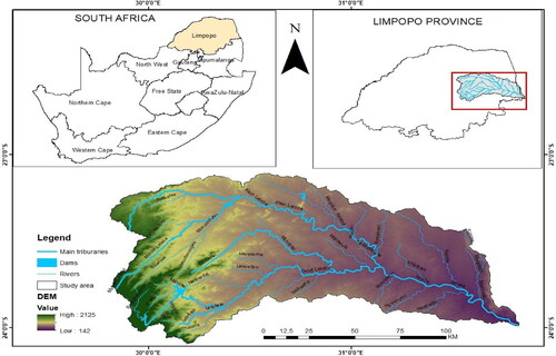
The study was conducted in the Letaba watershed situated between the longitudes 30°0′ and 31°40′ East and latitudes 23°30′ and 24°0′ South, in Limpopo province, South Africa (DWAF 2006) (Figure 1). The Letaba watershed covers the surface area of 1451864 ha. The area receives a mean annual evapotranspiration ranging from 1100 mm to 1300 mm, rainfall of 300 mm to 400 mm, annual runoff of 574 million m³ and the mean annual temperature ranges from the minimum 18° C to maximum of 28° C in the mountainous and in the lowlands respectively. The major tributaries of the Groot Letaba River which drained into the catchment are Klein Letaba, Middle Letaba, Molototsi and Litsetele rivers (DWAF 2006). The Letaba catchment has more than 20 constructed dams and weirs which resulted in the watershed being extremely regulated. The water resources that are available within the watershed are overexploited to meet the demand for domestic use and the need for commercial (afforestation, industry, and irrigation).

Figure 1. Location of the Letaba watershed, South Africa.

2.2. Field data

Field data collection for land cover types was conducted manually between February and March 2021, using handheld Garmin global positioning systems (GPS). The training dataset consisted of a total of one thousand and fifty (1050) ground truth points, with a hundred and fifty points allocated for each individual class. A balanced distribution strategy for class training samples was employed in the study. This approach was adopted to prevent any bias towards specific classes (Mellor et al. 2015). The use of balanced data distribution is associated with enhanced prediction accuracy and reliability across all classes (Mellor et al. 2015). The collected training data was converted into shapefile using ArcGIS, and subsequently imported into the GEE platform for the purpose of model training and validation for the LULC assessment of the Letaba watershed in 2021.

Similarly, high-resolution data from Google Earth was used to generate one thousand and fifty (1050) training data points serving as ground truth references for the year 1990. These points were then converted into shapefiles using ArcGIS and integrated into the GEE platform to facilitate the training of the LULC map for 1990. The same training dataset was further utilized for mapping LULC changes in the 2000 and 2010 images. In accordance with established standards in machine learning evaluation criteria, the imported training data areas were partitioned into two distinct sets: 70% for training and 30% for validation (Figure 2). As a result of this methodology, a comprehensive classification of seven distinct land cover types was executed within the confines of the Letaba watershed (Table 1).

Figure 2. the Schematic flow chart showing steps.

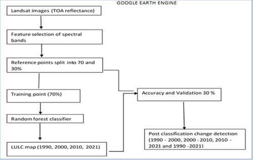
Table 1. Land use and land cover classification description.

Classes	Class no	Description
Bare surfaces (BS)	Class 5	Rocks, bare soil
Built-up (BU)	Class 2	Buildings, roads
Grasslands (GL)	Class 6	Rangelands
Natural Forests (NF)	Class 7	Dense, sparse
Plantations (PT)	Class 3	Tropical, pines, citrus
Water bodies (WB)	Class 4	Dams, rivers, streams
Shrublands (SL)	Class 8	Short trees

2.3. Data acquisition and processing

The Landsat 5 Top of Atmosphere (TOA) reflectance products, denoted as LT05/C01/T1_TOA, were utilized for the years 1990, 2000, and 2010. Similarly, Landsat 8 TOA reflectance products, identified as LC08/C01/T1_TOA, were employed for the year 2021. These data resources are available within the Google Earth Engine (GEE) cloud database, accessible via this link: https://earthengine.google.com/. Both Landsat 5 and Landsat 8 platforms encompass 7 and 13 spectral bands respectively, each with a spatial resolution of 30 meters. The TOA reflectance values for each spectral band within the GEE database were used in this study. To mitigate the impact of clouds and shadows, the cloud filtering function (QA_PIXEL) was applied, resulting in the removal of these unwanted elements from all filtered images. The process of filtering and creating mosaics was executed using the ‘filter’ function. The date parameters (start and end) were set to cover the periods from January 1st to December 31st for all four respective time intervals. Furthermore, the filtered images were cropped to match the boundaries of the study area through the utilization of the ‘filter.Bound()’ function. The resulting stacked images underwent normalization to account for illumination variations and to minimize the presence of clouds. Inclusion criteria for images involved selecting those with less than 20% cloud cover, except for the 2010 image, for which conditions necessitated the use of images with less than 50% cloud cover due to climatic considerations. The images were enhanced and smoothed to produce quality results.

2.4. Predictor variables

Within the GEE platform, the random forest (RF) algorithm was employed to identify the most influential spectral bands from Landsat images. This selection process was important for the prediction and mapping of LULC across the Letaba watershed. Utilizing this technique, researchers aimed to reduce the redundancy within explanatory variables (Dube et al. 2014; Mudereri et al. 2020).

2.5. Image classification and accuracy assessment

Google Earth Engine (GEE) provides a range of supervised classifiers, including the classification and regression tree (CART), support vector machine (SVM), Naive Bayes (NB), and Random Forest (RF). All four of these classifiers were tested for their effectiveness in categorizing LULC changes within the Letaba watershed. Following testing, the RF classifier emerged as the most superior performer among these options. As a result, it was subsequently utilized to map the dynamics of LULC within the Letaba Watershed. Support for this decision was also drawn from existing literature. The RF classifier available in GEE (ee.classifier.smileRandomForest) has consistently demonstrated outstanding performance in LULC classification when compared to CART, SVM, and NB, as attested by Abijith and Saravanan (2022), Gxokwe et al. (2022), and Kulithalai Shiyam Sundar and Deka (2022). Therefore, the algorithm was selected in this study because of its robustness and predictive accuracy even when applied to analyze data with strong noise (Zurqani et al. 2018).

The RF classifier is a non-parametric algorithm that constructs an ensemble model of decision trees from a random subset of features and a bagging randomisation process. RF has a greater processing power for data noise; overfitting and can work well with complex data with high accuracy (Piao et al. 2021). The classifier uses random sample data to generate multiple decision trees independently. The best node of each decision tree relies on a randomly selected subset of input prediction variables (Zhao et al. 2021). The process continues until the samples are similar and splitting no longer occurs. The final class prediction is chosen using the majority voting of the decision tree.

For LULC classification, accuracy assessment is imperative to explain the agreement between the ground truth and the classification outcome. To evaluate the classification accuracy for the year 2021, a subset of four hundred and twenty (420) reference points (representing 30% of the dataset) was used. Similarly, for the year 1990, 2000, and 2010 a total of four hundred and twenty (420) was also used for validation of the accuracy. The validation dataset was employed to generate a confusion matrix within GEE for accuracy assessment. The assessment metrics encompass producer accuracy (PA), overall accuracy (OA), and user accuracy (UA), with the exclusion of Kappa due to its criticized suitability for accuracy assessment (Pontius and Millones 2011).

2.6. Land use change detection

The method of post-classification was employed to determine the magnitude trend and rate of LULC change within Letaba watershed. An analysis of area comparison was conducted by subtracting the total area for each class, resulting in both positive (increasing) and negative (decreasing) values. The percentage and rate of LULC change were calculated using the subsequent formulas:

The proportion of each LULC class type Ai = Ai/At *100

The change for each LULC class type was computed as follows: Ai = Ait₁ - Ait₂ and the

Annual rate of change: Air = ((Ait₁/Ait₂)-1) *100%

In these formulas, i represents the particular area of the LULC class type, At designates the total study area, and Ai % denotes the proportion of each LULC class area. Ait₁ and Ait₂ refers to the total area of LULC class type in specific years ₁ and ₂ respectively (Lu et al. 2013; Piao et al. 2021). Air refers to the rate of change, which magnitude of change between the specified years and the range of change from 1990 to 2021 was analysed (Piao et al. 2021; Tian et al. 2014). Notably, this method offers the advantage of providing insights into both magnitude and direction of change, while also indicating the number of areas that have undergone alterations.

3. Results

3.1. Variables of importance

The RF classifier implemented within GEE was used to train the sample with settings of 100 decision trees in mapping LULC in Letaba watershed. The RF classifier demonstrated a notably overall high level of accuracy in effectively identifying and delineating various LULC categories across the watershed. The spectral bands of Landsat images, specifically band 2 (blue), band 5 (near-infrared or NIR), and band 6 (shortwave-infrared or SWIR), were identified as the most crucial variables for the RF classification process (Figure 3). These specific bands were chosen to predict LULC classes for the years 1990, 2000, 2010, and 2021. This selection served purpose of minimizing data redundancy among explanatory variables and enhancing the classification precision.

Figure 3. Variables of importance percentage derived using the RF variable selection method.

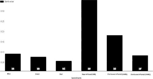
The cloud-based methodology adopted for this study revealed a notable capability to accurately define LULC classes, offering a visual representation that effectively covered the majority of classes present within the Letaba watershed. In order to optimize the predictive performance, less significant variables were omitted from consideration, as they did not contribute meaningfully to the prediction process. The selection of valuable bands was able to distinguish classes from one another and increased the classification accuracy of the study area

3.2. Land cover and land use classification and accuracy

The RF classifier successfully distinguished LULC classes, achieving OA of 0.95, 0.97, 0.93 and 0.99 for the year 1990, 2000, 2010 and 2021 respectively (Table 2). UA and PA values, derived from the confusion matrix, were computed for each class type across all years. Plantations and natural forests occurred in close proximity; however, the RF model effectively captured variations in the upstream area of the Letaba watershed. Notably, the class with the highest accuracy was shrublands, exhibiting a perfect 100% with PAs, and UAs ranging between 93% and 97% across all time periods. Likewise, water bodies were accurately classified, with PAs ranging from 92% to 98%, and UAs ranging from 95% to 100%. Comparatively, lower classification accuracies were achieved for the Natural Forest class, with PAs varying from 83% to 100% across all time frames. Regarding error assessment, the 2021 classification showcased lower values for error commission (EC) and error of omission (ER), ranging between 0% and 5%. Conversely, the classification for 1990 exhibited higher values of ER (14%) and EO (12%) respectively.

Table 2. Derived LULC error matrix for the year 1990, 2000, 2010 and 2021.

1990	BS	BU	GL	NF	PT	WB	SL	Total	UA	EC
BS	60	0	0	0	0	0	0	60	100.00	0
BU	0	60	0	0	0	0	0	60	100.00	0
GL	1	0	59	0	0	0	0	60	98.33	2
NF	2	0	0	55	1	2	0	60	91.67	8
PT	2	0	1	4	53	0	0	60	88.33	12
WB	2	0	0	1	0	57	0	60	95.00	5
SL	3	0	0	0	1	0	56	60	93.33	7
Total	70	60	60	60	55	59	56	420
PA	85.71	100.00	98.33	91.67	96.36	96.61	100.00
EO	14	0	2	8	2	3	0
		OA	95.24
2000	BS	BU	GL	NF	PT	WB	SL	Total	UA	EC
BS	60	0	0	0	0	0	0	60	100.00	0
BU	1	59	0	0	0	0	0	60	98.33	2
GL	1	1	56	1	0	1	0	60	93.33	7
NF	0	0	0	60	0	0	0	60	100.00	0
PT	2	0	0	3	55	0	0	60	91.67	8
WB	0	0	0	1	0	59	0	60	98.33	2
SL	1	0	0	1	0	0	58	60	96.67	3
Total	65	60	56	66	55	60	58	420
PA	92.31	98.33	100.0	90.91	100.0	98.33	100.00
EO	8	2	0	9	0	2	0
		OA	96.90
2010	BS	BU	GL	NF	PT	WB	SL	Total	UA	EC
BS	59	0	0	0	0	1	0	60	98.33	2
BU	4	56	0	0	0	0	0	60	93.33	7
GL	0	0	56	2	0	2	0	60	93.33	7
NF	0	0	0	57	1	2	0	60	95.00	5
PT	3	0	0	7	50	0	0	60	83.33	17
WB	0	0	0	3	0	57	0	60	95.00	5
SL	0	0	2	0	1	0	57	60	95.00	5
Total	66	56	58	69	52	62	57	420
PA	89.39	100.00	96.55	82.61	96.15	91.94	100
EO	11	0	3	7	4	5	0
		OA	93.33
2021	BS	BU	GL	NF	PT	WB	SL	Total	UA	EC
BS	57	3	0	0	0	0	0	60	95.00	5
BU	0	60	0	0	0	0	0	60	100.00	0
GL	0	0	60	0	0	0	0	60	100.00	0
NF	0	0	0	60	0	0	0	60	100.00	0
PT	0	0	0	0	60	0	0	60	100.00	0
WB	0	0	0	0	0	60	0	60	.00	0
SL	2	0	0	0	0	0	58	60	96.67	3
Total	61	65	60	60	60	60	58	420
PA	96.72	92.31	100.0	100.0	100.00	100.0	100
EO	3	5	0	0	0	0	0
		OA	98.80

3.3. The spatiotemporal changes of the Letaba watershed in 31 years

Over the past 31 years, significant shifts in land use and land cover (LULC) have been observed within the Letaba watershed (Figure 4, Table 3). By the year 2021, there has been noteworthy transformation in the LULC composition. Particularly, the natural forests and grasslands have undergone deforestation and degradation, resulting in a decline in their respective percentage covers from 13% and 23% in 1990 to 6% and 9% in 2021. Furthermore, there has been a reduction in the percentage cover of bare surfaces and water bodies, which decreased from 44% and 13% in 1990 to 29% and 1% in 2021, respectively. In contrast, there has been a considerable increase in the percentage covers of plantations, shrublands, and built-up areas. These categories have seen their coverage expand from 4%, 2%, and 2% in 1990 to 24%, 15%, and 16% in 2021, respectively.

Figure 4. Spatiotemporal pattern of LULC at Letaba watershed.

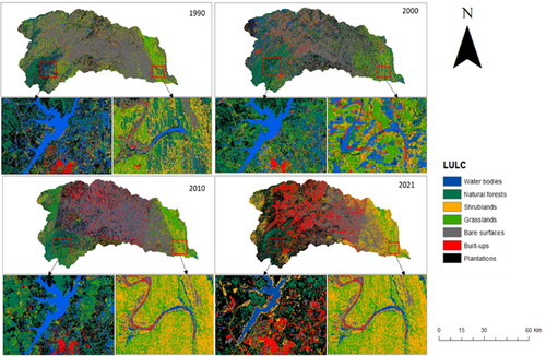
Table 3. Area covered by each class type for four-time period.

	1990		2000		2010		2021
Classes	Area (ha)	Area (%)	Area (ha)	Area (%)	Area (ha)	Area (%)	Area (ha)	Area (%)
Bare Surfaces	645894	44	581998	40	560638	39	418694	29
Built Up	22068	2	47395	3	140123	10	238994	16
Grasslands	335100	23	193814	13	194121	13	134894	9
Water bodies	184736	13	99332	7	106812	7	15595	1
Natural Forests	184049	13	170381	12	142161	10	84325	6
Plantations	57514	4	277227	19	216961	15	343700	24
Shrublands	22503	2	81717	6	91048	6	215662	15
Total	1451864	100	1451864	100	1451864	100	1451864	100

The rate of change revealed different changing progression for each class category from 1990 to 2021 refer to Table 4. Bare surfaces, water bodies, natural forest and grasslands areas reduced trend at a rate of −2%, −4%, −3% and −3% respectively whereby plantations area increased at rate of 24%. However, built-up and shrublands showed a clear extension trend which significantly increased from the year 1990 to 2021 with a rate of 47% and 41% respectively. The highest intensity of built-up area and plantations occurred between 1990 and 2021, and for shrublands occurred between 2010 and 2021 (Figure 5). Conversely, the highest decline intensity of water bodies, natural forests and bare surfaces occurred between 2010 and 2021, and grassland occurred in two time periods between the year 2000 and 2010 and 1990 and 2021.

Figure 5. Representation of total area LULC change (gains and loss) on Letaba watershed for the time period 1990, 2000, 2010 and 2021.

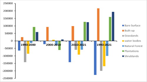
Table 4. the rate of change in LULC classes from the year 1990 to 2021.

Class	1990 Area %	2021 Area %	1990–2021 rate of change %
Bare surfaces	44	29	−2
Built-up	2	16	47
Grasslands	23	9	−3
Water bodies	13	1	−4
Natural forests	13	6	−3
Plantations	4	24	24
Shrublands	2	15	41

Moreover, the study revealed a reduction in the area covered by natural forest to plantations in the upstream of the watershed. Whereas grasslands are hastily replaced by shrublands downstream of the watershed. The bare surfaces are swiftly substituted by built-up and plantations in the middle stream of the watershed. Although bare surfaces areas are decreasing and are still the most dominating land cover in the watershed. The water bodies are diminished by plantations and construction of dams alongside the streams in the middle and upper streams which prevents the flow of the water downstream of the watershed. Additionally, water bodies downstream of the watershed are becoming drier and converted into bare surfaces.

4. Discussion

Accurate detection and mapping of LULC are important for understanding the drivers that results in change of the natural environment into human dominant. Advanced data analytics and remote sensing application has improved fast monitoring of LULC changes in Letaba watershed. The implementation of GEE has been effective for leveraging big data in remote sensing technology. This technology allows users from other regions to adapt and customize the existing analysis scripts or create new ones that cater to the specific characteristics of the new region (Huang et al. 2017). This may include modifying classification algorithms, adjusting parameters, and thresholds based on the unique land cover types, climate, and land use patterns (Azzari and Lobell 2017).

The aim of this study was to determine the spatiotemporal changes in LULC within the Letaba watershed from 1990 to 2021 using GEE. The scalability and flexibility of GEE's platform demonstrated the capabilities in continuous monitoring LULC changes and support targeted management and conservation strategies across diverse landscapes and regions (Pan et al. 2022). The limitations of GEE include spatial and temporal resolutions of satellite image, which may not be adequate for capturing fine-scale changes in a heterogeneous landscape. This can lead to challenges in accurately identifying and classifying different land cover types, in areas with complex and mixed land use patterns. Cloud cover can be a significant issue in tropical regions, this can limit the availability of cloud-free imagery, which affects the temporal consistency and reliability of LULC change detection (Delalay et al. 2019). Additionally, GEE's algorithms and processing methods might not be optimized for the specific characteristics and challenges of mapping LULC changes in watersheds. GEE might perform well in certain regions but may lack accuracy and generalization when applied to complex and heterogeneous semi-arid landscapes (Gxokwe et al. 2022). The interpretation of LULC changes requires careful consideration of local socio-economic and cultural factors. GEE's remote sensing approach might not fully capture the drivers and underlying reasons for LULC changes, limiting the understanding of the complexities involved.

Based on the analysis using the GEE the use of RF for classification provided useful information in detecting and mapping spatiotemporal changes of the Letaba watershed. The results from the RF analysis demonstrated the efficacy of utilizing specific spectral band values to differentiate various land cover classes present in the watershed. Notably, the Blue, Near-Infrared (NIR), and Shortwave Infrared 1 (SWIR1) bands exhibited significant discriminatory power among these classes (Mudereri et al. 2020). Among these bands, the NIR band emerged as the most pivotal due to its sensitivity to factors like vegetation type, water content, density, and overall vegetation health (Forkuor et al. 2018; Kyere et al. 2019). Likewise, the SWIR1 band’s sensitivity to moisture levels and shades in the forest stand structure proved valuable in the classification process (Izadi and Sohrabi 2021). Additionally, the Blue band played a crucial role in distinguishing between soil and vegetation, as well as differentiating deciduous trees from coniferous vegetation (Acharya and Yang 2015; Zeferino et al. 2020).

The study’s findings also suggested that a strategic selection of a few informative bands could potentially outperform the classification achieved using the entire set of wavebands (Cai et al. 2018; Dube and Mutanga 2015; Mudereri et al. 2020). While the spectral bands alone demonstrated the capability to differentiate land cover, the incorporation of indices such as the Normalized Difference Vegetation Index (NDVI), Modified Normalized Difference Water Index (NDWI), Normalized Difference Built-Up Index (NDBI), and slope could potentially provide additional value in the prediction and mapping of LULC (Tolentino and Galo 2021). Despite RF's success in effectively mapping LULC within the Letaba area, it’s important to acknowledge certain limitations associated with the classifier. When dealing with datasets characterized by imbalanced class distributions, RF might exhibit a bias towards the majority class, potentially resulting in decreased accuracy for minority classes and the risk of overfitting (Pan et al. 2022).

The information regarding precision and accuracy presented in the classified map outcomes holds significant importance for users aiming to effectively utilize the generated maps (Munthali et al. 2019). Therefore, conducting accuracy assessment remains a pivotal step in image classification, and this study demonstrated commendable accuracy results, even though some errors arose from spectral confusion among natural forests, bare surfaces, and plantations. The established standard level for overall classification accuracy typically stands at 85% (Yesuph and Dagnew 2019). However, the outcomes of this study outperformed this standard, achieving remarkable overall accuracy rates of 95%, 97%, 93%, and 99% for the years 1990, 2000, 2010, and 2021 respectively. This achievement indicates that the classification results were both rational and dependable, enabling subsequent post-classification change detection comparisons. The high overall accuracy achieved can be implementation of the RF classifier, which effectively minimize errors as the number of decision trees increases (Abijith and Saravanan 2022), and the selection of variable importance reduces the redundancy of correlated variables. It is essential to note that the accuracy of LULC classification within the GEE depends on the availability of high-quality training data.

Utilizing ground truth data has proven to be effective in achieving high classification accuracy within the Letaba watershed. Nonetheless, the challenges associated with acquiring ground truth data for validation can be difficult in remote and inaccessible areas. This can result in potential inaccuracies during the classification procedure and minimize confidence in the outcomes. Xiong et al. 2017 automated crop mapping using GEE. This method can quickly generate training data, enabling rapid response to changing land cover conditions, and provide consistent training samples across the study area, reducing potential bias (Verde et al. 2020; Xiong et al. 2017). Automated methods are useful when you need to quickly classify large areas or monitor changes frequently.

They work well in situations where ground truth data are scarce or when capturing rapid changes is crucial. Although automated methods in GEE provides an impressive computational infrastructure; it still relies on remote sensing data and may not be a substitute for detailed on-the-ground surveys and local knowledge (Pan et al. 2022). Field-based data collection and ground-truthing are essential for validating and improving the accuracy of LULC maps generated through GEE (Kandekar et al. 2021). Automated and field-based data collection methods share the common objective of enhancing accuracy in land cover analysis. Both approaches contribute to reliable classification outcomes by providing representative training samples. Automated methods leverage algorithms to rapidly generate training points from spectral properties, enabling efficient processing of large datasets (Zhang et al. 2021). In contrast, field-based data collection involves on-site observations, capturing contextual details that algorithms might miss (Pande et al. 2018).

The process and rate of change over the 31 years were analysed using four time periods with rapid increase in shrublands and built-up from 2% and 2% in 1990 to 15% and 16% in 2021 respectively. The increase rate (47%) in the built-up areas (residential, commercial, roads, and industries) could be attributed to increasing demand for land by growing population rate and development of commercial infrastructure that are taking place in the Letaba watershed (DWAF 2004; Querner et al. 2016). Such expansion of buildings transforms natural landscape which emerge to severe environmental such as loss of natural habitat. This disrupts the connectivity between ecosystems, isolating populations of plants and animals and reducing genetic diversity, making species more vulnerable to extinction (Hailu et al. 2021). The increased impervious surface such as pavements, reduce natural water infiltration, leading to increased surface runoff during rainfall events. This can result in water pollution as runoff carries pollutants from urban areas into nearby water bodies, negatively impacting aquatic ecosystems and biodiversity (Du Plessis et al. 2014; Namugize et al. 2018).

Moreover, the plantations also increased from 4% in 1990 to 24% in 2021, which indicates that plantations are the main source of income within the watershed. The increase rate (24%) of plantations in the Letaba watershed can be attributed to rapid growth in demand for arable land (Marks-Bielska and Witkowska-Dabrowska 2021). The expansion of uncontrollable plantation lands often results in deforestation, wetland conversion, or the draining of natural habitats to make way for crops or livestock. This leads to habitat loss and fragmentation, disrupting ecosystems and reducing biodiversity as native species struggle to adapt or face displacement. The intensification of plantations using agrochemicals, irrigation, and monoculture practices can lead to soil degradation, erosion, and loss of fertility. This do not only affect agricultural productivity but also impacts nearby water bodies through runoff of pesticides and fertilizers, leading to water pollution and harming aquatic life (Chen et al. 2014; Uniyal et al. 2020). The population increase has resulted in conversion of bare surfaces and grasslands into built-up areas from the year 1990 to 2021.

The decrease rate (−3%) of grassland could be attributed to overgrazing, encroaching invasive tree species which suppress the growth of grasslands and the effects of climate change. The decreasing grassland will have implications on the functioning of ecosystems in the area, climate regulation and depletion of species (Ceballos et al. 2010; Zavaleta and Hulvey 2004). Grasslands play a crucial role in providing ecosystem services such as carbon sequestration, water filtration, and soil conservation. Their destruction can release stored carbon into the atmosphere, reduce water quality due to increased runoff, and lead to soil erosion (Wang et al. 2022).

The bushes are encroaching the grasslands with an increase rate of 41%. The invasion of bushes could be attributed to veld fires and climate change effects downstream of the Letaba watershed. The invasion will also alter the vegetation structure and water use characteristics in ways which can reduce the runoff or decrease the groundwater recharge and results in loss of biodiversity (Le Maitre et al. 2020). The findings of grassland being converted to bushlands correspond with the study by Yesuph and Dagnew (2019) at the Beshilo Catchment in Ethiopia. The increased rate of shrub encroachment can fragment and disrupt natural ecosystems. The formation of dense shrub patches may act as barriers to the movement of wildlife, making it difficult for some species to access food, water, or breeding sites (Shiferaw et al. 2019). This fragmentation can reduce gene flow and genetic diversity within populations, potentially leading to inbreeding and reduced resilience to environmental changes (Wang et al. 2022).

Comparatively, the decline rate (- 4%) of water bodies can be attributed to the significant increase in the plantations along the river and streams, invasive species and lots of constructed dams and weirs within the watershed which is becoming a problematic (Pullanikkatil et al. 2016; Munthali et al. 2019). This relates with the study by Munthali et al. (2019) in Dedza district of Malawi where they observed an increase in plantation alongside the stream at the expense of the water bodies. The reduction of water bodies leads to degraded water quality, loss of critical ecosystem services like water purification and flood regulation, and increased vulnerability to climate change impacts. This threatens the livelihoods of local communities’ dependent on fisheries and agriculture, while also impacting the overall health and resilience of surrounding terrestrial ecosystems (Rotich et al. 2022).

The study also revealed that natural forests deteriorated from (13%) in 1990 to (6%) in 2021 in the upper watershed. The declining rate (−3%) of natural forest cover could be attributed to the rapid population growth in demand for arable land for food production as it is mostly converted into plantations. The result corresponds with the finding by Agariga et al. (2021) where they observed conversion of forest to agriculture between 1986 and 2020. The decline in natural forest also reduces the size of the carbon sinks, thereby contributing to greenhouse gas emissions (Berry et al. 2010). Bare surface decreased from 44% in 1990 to 29% in 2021 with a decreased rate of −2%. Most of the bare surfaces were converted into built-up and plantations.

The changes in LULC within the Letaba are driven by lack regulations, policies, and socioeconomic factors. Therefore, It is essential to understand these drivers and policy contexts behind LULC changes to develop effective strategies for sustainable land management, biodiversity conservation, and environmental protection. Integrating environmental considerations into policy-making processes can help balance human development needs with conservation goals and foster sustainable land use practices (Rotich et al. 2022). The information gathered from this study can be used to develop targeted management strategies to address challenges such declined water bodies, grasslands, and natural forest and promote sustainable land use practices. To manage the socioeconomic implications of LULC changes in Letaba watershed effectively, it is crucial to integrate social considerations into land use planning and decision-making processes. Community engagement, participatory approaches, and consideration of local knowledge can help ensure that the interests and well-being of the local population are considered in development and conservation initiatives. Moreover, balancing economic development with environmental sustainability is essential for promoting the long-term prosperity and resilience of local communities.

Conclusion

With the right set of variables, the GEE's RF classifier can accurately map and predict the extent and rate of LULC dynamics. The findings revealed that the Letaba watershed experienced significant LULC change between 1990 and 2021. During these years, the watershed has lost bare surfaces, water bodies, grassland, and natural forest. While built-up, shrublands and plantations are on the rise. Built-up, plantations and shrublands are likely to continue growing due to the growing population’s demand for settlement and arable land to meet human needs, as well as climate change variability favouring invasive shrubland. Water bodies, natural forests, bare surfaces, and grassland are also expected to decline further as a result of overexploitation of water for irrigation of commercial farming within the Letaba catchment, rapidly increasing population, and invasive shrub species. The lack of enforced regulation and policies to protect natural resources within the Letaba watershed is the primary driver of the large LULC transition. The majority of natural forest conversion to plantation areas will result in deforestation, which will have consequences for ecosystems, human livelihoods, climate regulation, and biodiversity. Grasslands, on the other hand, are being converted to shrublands, built-up areas, and plantations, which has implications for the extinction of uncounted populations and species, as well as biodiversity and climate. As a result, environmentalists, watershed managers, forest managers, decision makers, and stakeholders must act quickly to address issues of environmental degradation. To avoid land degradation, the study recommends that appropriate measures be taken to protect and restore natural resources such as grasslands, natural forests, water bodies, and eradicate invasive shrubs in the Letaba watershed.

Disclosure statement

No potential conflict of interest was reported by the authors.

Appendix

The code used in GEE to produce LULC maps and accuracy within the study area

paravar visParamsTrue = {bands: ['B3', 'B2', 'B1']}; var visParamsTrue2 = {bands: ['B4', 'B3', 'B2']}; var training = ee.FeatureCollection("users/makgabomashala/LC-2021"); var geometry = ee.FeatureCollection("users/makgabomashala/Letaba") var L5 = ee.ImageCollection("LANDSAT/LT05/C02/T1_TOA") var L8 = ee.ImageCollection("LANDSAT/LC08/C02/T1_TOA")

Map.addLayer(training, {}, 'raw_data’,true); function maskLandsatclouds(image) { var qa = image.select('QA_PIXEL') var cloudBitMask = ee.Number(2).pow(4).int() var mask = qa.bitwiseAnd(cloudBitMask).eq(0) return image.updateMask(mask) .select("B.*") .copyProperties(image, ["system:time_start"]) } var L8image2 = L8.filterDate('2021-01-01′, '2021-12-31′)//you can change date here .filter(ee.Filter.lt("CLOUD_COVER", 20)) .filterBounds(geometry) .map(maskLandsatclouds) .select('B.*'); var image2 = L8.median().clip(geometry);//here we are taking the median at each pixel in the collection

Map.addLayer(image2,visParamsTrue2, "mosaic_L8"); print(image2); var L5image = L5.filterDate('1990-01-01′, '1990-12-31′)//you can change date here .filter(ee.Filter.lt("CLOUD_COVER", 20)) .filterBounds(geometry) .map(maskLandsatclouds) .select('B.*'); var image = L5.median().clip(geometry);// Map.addLayer(image, visParamsTrue, "mosaic_L5"); print(image); var data = ee.FeatureCollection(training, 'geometry’); var datawithColumn = data.randomColumn('random’); print('datawithColumn’,datawithColumn) var split = 0.70;//separate 70% for training, 30% for validation var trainingData = datawithColumn.filter(ee.Filter.lt('random’, split)); var validationData = datawithColumn.filter(ee.Filter.gte('random’, split)); print('trainingData’, trainingData) print('validationData’, trainingData) var bands = image.bandNames(); var bands2 = image2.bandNames(); print('bands’,bands) print('bands2',bands2) var training = image.select(bands).sampleRegions({ collection: trainingData, properties: ['LC'], scale: 30 }); var training = image2.select(bands2).sampleRegions({ collection: trainingData, properties: ['LC'], scale: 30, tileScale: 16 }); var classifier = ee.Classifier.smileRandomForest(500, null, 2, 0.5, null, 0) .setOutputMode('CLASSIFICATION') .train({ features: training, classProperty: 'LC', inputProperties: bands }); var classified = image.select(bands).classify(classifier); var classified2 = image2.select(bands2). classify(classifier); Map.addLayer(classified) Map.addLayer(classified2) var trainAccuracy = classifier.confusionMatrix(); print('Training overall accuracy:', trainAccuracy.accuracy()); print('validation accuracy:', trainAccuracy.accuracy()); print('error matrix:', trainAccuracy);//Confusion matrix var dict = classifier.explain(); print("Classifier information:", dict); var variableImportance = ee.Feature(null, ee.Dictionary(dict).get('importance’)); var chart =  ui.Chart.feature.byProperty(variableImportance) .setChartType('ColumnChart’) .setOptions({ title: 'Random Forest Variable Importance’, legend: {position: 'none’}, hAxis: {title: 'Bands’}, vAxis: {title: 'Importance’} }); print(chart); var options = { lineWidth: 1, pointSize: 2, hAxis: {title: 'Classes’}, vAxis: {title: 'Num of pixels’}, title: 'Number of pixels in each class’ };

References

- Abijith D, Saravanan S. 2022. Assessment of land use and land cover change detection and prediction using remote sensing and CA Markov in the northern coastal districts of Tamil Nadu, India. Environ Sci Pollut Res. 29(57):86055–86067.
- Acharya TD, Yang I. 2015. Exploring landsat 8. Int J IT, Eng Appl Sci Res (IJIEASR). 4(4):4–10.
- Agariga F, Abugre S, Appiah M. 2021. Spatio-temporal changes in land use and forest cover in the Asutifi North District of Ahafo Region of Ghana, (1986–2020). Environ Chall. 5:100209. doi: 10.1016/j.envc.2021.100209.
- Alemayehu F, Taha N, Nyssen J, Girma A, Zenebe A, Behailu M, Deckers S, Poesen J. 2009. The impacts of watershed management on land use and land cover dynamics in Eastern Tigray (Ethiopia). Resour Conserv Recycl. 53(4):192–198. doi: 10.1016/j.resconrec.2008.11.007.
- Amsalu A, Stroosnijder L, de Graaff J. 2007. Long-term dynamics in land resource use and the driving forces in the Beressa watershed, highlands of Ethiopia. J Environ Manage. 83(4):448–459. doi: 10.1016/j.jenvman.2006.04.010.
- Azzari G, Lobell DB. 2017. Landsat-based classification in the cloud: an opportunity for a paradigm shift in land cover monitoring. Remote Sens Environ. 202:64–74. doi: 10.1016/j.rse.2017.05.025.
- Berry NJ, Phillips OL, Lewis SL, Hill JK, Edwards DP, Tawatao NB, Ahmad N, Magintan D, Khen CV, Maryati M, et al. 2010. The high value of logged tropical forests: lessons from northern Borneo. Biodivers Conserv. 19(4):985–997. doi: 10.1007/s10531-010-9779-z.
- Bufebo B, Elias E. 2021. Land use/land cover change and its driving forces in Shenkolla watershed, south Central Ethiopia. Sci World J. 2021:1–13. doi: 10.1155/2021/9470918.
- Cai J, Luo J, Wang S, Yang S. 2018. Feature selection in machine learning: a new perspective. Neurocomputing. 300:70–79. doi: 10.1016/j.neucom.2017.11.077.
- Ceballos G, Davidson A, List R, Pacheco J, Manzano-Fischer P, Santos-Barrera G, Cruzado J. 2010. Rapid decline of a grassland system and its ecological and conservation implications. PLoS One. 5(1):e8562. doi: 10.1371/journal.pone.0008562.
- Chaves ME, Soares AR, Mataveli GA, Sánchez AH, Sanches ID. 2023. A semi-automated workflow for lulc mapping via sentinel-2 data cubes and spectral indices. Automation. 4(1):94–109. doi: 10.3390/automation4010007.
- Chen Y, Shuai J, Zhang Z, Shi P, Tao F. 2014. Simulating the impact of watershed management for surface water quality protection: a case study on reducing inorganic nitrogen load at a watershed scale. Ecol Eng. 62:61–70. doi: 10.1016/j.ecoleng.2013.10.023.
- Cui J, Zhu M, Liang Y, Qin G, Li J, Liu Y. 2022. Land use/land cover change and their driving factors in the Yellow River Basin of Shandong Province based on google earth Engine from 2000 to 2020. IJGI. 11(3):163. doi: 10.3390/ijgi11030163.
- de Sousa MDC, Veloso GV, Gomes LC, Fernandes-Filho EI, de Oliveira TS. 2021. Spatio-temporal dynamics of land use changes of an intense anthropized basin in the Brazilian semi-arid region. Remote Sens Appl: Soc Environ. 24:100646. doi: 10.1016/j.rsase.2021.100646.
- Delalay M, Tiwari V, Ziegler AD, Gopal V, Passy P. 2019. Land-use and land-cover classification using Sentinel-2 data and machine-learning algorithms: operational method and its implementation for a mountainous area of Nepal. J Appl Rem Sens. 13(01):1. doi: 10.1117/1.JRS.13.014530.
- Du Plessis A, Harmse T, Ahmed F. 2014. Quantifying and predicting the water quality associated with land cover change: a case study of the Blesbok Spruit Catchment, South Africa. Water. 6(10):2946–2968. doi: 10.3390/w6102946.
- Dube T, Mutanga O. 2015. Evaluating the utility of the medium-spatial resolution Landsat 8 multispectral sensor in quantifying aboveground biomass in uMgeni catchment, South Africa. ISPRS J Photogramm Remote Sens. 101:36–46. doi: 10.1016/j.isprsjprs.2014.11.001.
- Dube T, Mutanga O, Adam E, Ismail R. 2014. Intra-and-inter species biomass prediction in a plantation forest: testing the utility of high spatial resolution spaceborne multispectral rapideye sensor and advanced machine learning algorithms. Sensors (Basel). 14(8):15348–15370. doi: 10.3390/s140815348.
- DWAF. 2004. Internal Strategic Perspective: luvuvhu/Letaba Water Management Area. Report No. PWMA 02/000/00/0304. Pretoria, South Africa: Department of Water Affairs and Forestry.
- DWAF. 2006. Letaba catchment reserve determination study. February 2006. Pretoria, South Africa: department of Water Affairs and Forestry.
- Forkuor G, Dimobe K, Serme I, Tondoh JE. 2018. Landsat-8 vs. Sentinel-2: examining the added value of sentinel-2’s red-edge bands to land-use and land-cover mapping in Burkina Faso. GIScience Remote Sens. 55(3):331–354. doi: 10.1080/15481603.2017.1370169.
- Gorelick N, Hancher M, Dixon M, Ilyushchenko S, Thau D, Moore R. 2017. Google Earth Engine: planetary-scale geospatial analysis for everyone. Remote Sens Environ. 202:18–27. doi: 10.1016/j.rse.2017.06.031.
- Grecchi RC, Gwyn QHJ, Bénié GB, Formaggio AR, Fahl FC. 2014. Land use and land cover changes in the Brazilian Cerrado: a multidisciplinary approach to assess the impacts of agricultural expansion. Appl Geogr. 55:300–312. doi: 10.1016/j.apgeog.2014.09.014.
- Gxokwe S, Dube T, Mazvimavi D. 2022. Leveraging Google Earth Engine platform to characterize and map small seasonal wetlands in the semi-arid environments of South Africa. Sci Total Environ. 803:150139. doi: 10.1016/j.scitotenv.2021.150139.
- Hailu S, Tena A, Tibebu K, Gete Z. 2021. Evaluating ecosystems services values due to land use transformation in the Gojeb watershed, Southwest Ethiopia. Environ Syst Res. 10(1).
- Hoque MZ, Islam I, Ahmed M, Hasan SS, Prodhan FA. 2022. Spatio-temporal changes of land use land cover and ecosystem service values in coastal Bangladesh. Egypt J Remote Sens Space Sci. 25(1):173–180. doi: 10.1016/j.ejrs.2022.01.008.
- Huang H, Chen Y, Clinton N, Wang J, Wang X, Liu C, Gong P, Yang J, Bai Y, Zheng Y, et al. 2017. Mapping major land cover dynamics in Beijing using all Landsat images in Google Earth Engine. Remote Sens Environ. 202:166–176. doi: 10.1016/j.rse.2017.02.021.
- Izadi S, Sohrabi H. 2021. Using Bayesian kriging and satellite images to estimate above-ground biomass of Zagros mountainous forests. In Forest resources resilience and conflicts. Amsterdam, The Netherlands: Elsevier; p. 193–201.
- Jansen LJ, Di Gregorio A. 2002. Parametric land cover and land-use classifications as tools for environmental change detection. Agric Ecosyst Environ. 91(1-3):89–100. doi: 10.1016/S0167-8809(01)00243-2.
- Kandekar VU, Pande CB, Rajesh J, Atre AA, Gorantiwar SD, Kadam SA, Gavit B. 2021. Surface water dynamics analysis based on sentinel imagery and Google Earth Engine Platform: a case study of Jayakwadi dam. Sustain Water Resour Manag. 7(3):44. doi: 10.1007/s40899-021-00527-7.
- Kerr J, Chung K. 2002. Evaluating watershed management projects. Water Policy. 3(6):537–554. doi: 10.1016/S1366-7017(02)00016-8.
- Kombate A, Folega F, Atakpama W, Dourma M, Wala K, Goïta K. 2022. Characterization of land-cover changes and forest-cover dynamics in Togo between 1985 and 2020 from Landsat images using Google Earth Engine. Land. 11(11):1889. doi: 10.3390/land11111889.
- Kulithalai Shiyam Sundar P, Deka PC. 2022. Spatio-temporal classification and prediction of land use and land cover change for the Vembanad Lake system, Kerala: a machine learning approach. Environ Sci Pollut Res Int. 29(57):86220–86236. doi: 10.1007/s11356-021-17257-0.
- Kumar L, Mutanga O. 2018. Google Earth Engine applications since inception: usage, trends, and potential. Remote Sens. 10(10):1509. doi: 10.3390/rs10101509.
- Kyere I, Astor T, Graß R, Wachendorf M. 2019. Multi-temporal agricultural land-Cover mapping using single-year and multi-year models based on Landsat imagery and IACS data. Agronomy. 9(6):309. doi: 10.3390/agronomy9060309.
- Le Maitre DC, Blignaut JN, Clulow A, Dzikiti S, Everson CS, Görgens AH, Gush MB. 2020. Impacts of plant invasions on terrestrial water flows in South Africa. Biol Invasions S Afr:431–457. Cham: Springer International Publishing.
- Lee JSH, Wich S, Widayati A, Koh LP. 2016. Detecting industrial oil palm plantations on Landsat images with Google Earth Engine. Remote Sens Appl: Soc Environ. 4:219–224. doi: 10.1016/j.rsase.2016.11.003.
- Leta MK, Demissie TA, Tränckner J. 2021. Modeling and prediction of land use land cover change dynamics based on land change modeler (Lcm) in nashe watershed, upper blue nile basin, Ethiopia. Sustainability. 13(7):3740. doi: 10.3390/su13073740.
- Lin L, Hao Z, Post CJ, Mikhailova EA, Yu K, Yang L, Liu J. 2020. Monitoring land cover change on a rapidly urbanizing island using Google Earth Engine. Appl Sci. 10(20):7336. doi: 10.3390/app10207336.
- Liping C, Yujun S, Saeed S. 2018. Monitoring and predicting land use and land cover changes using remote sensing and GIS techniques—a case study of a hilly area, Jiangle, China. PLoS One. 13(7):e0200493. doi: 10.1371/journal.pone.0200493.
- Loukika KN, Keesara VR, Sridhar V. 2021. Analysis of land use and land cover using machine learning algorithms on Google Earth Engine for Munneru River Basin, India. Sustainability. 13(24):13758. doi: 10.3390/su132413758.
- Lu D, Li G, Moran E, Hetrick S. 2013. Spatiotemporal analysis of land-use and land-cover change in the Brazilian Amazon. Int J Remote Sens. 34(16):5953–5978. doi: 10.1080/01431161.2013.802825.
- Marks-Bielska R, Witkowska-Dabrowska M. 2021. Evaluation of changes in exclusion of arable land from agricultural production in Poland in the context of guidelines of the strategy for responsible development. ERSJ. XXIV(Special Issue 3):351–364. doi: 10.35808/ersj/2433.
- Mashala MJ, Dube T, Mudereri BT, Ayisi KK, Ramudzuli MR. 2023. An advancements in remote sensing for assessing and monitoring land use and land cover changes impacts on surface water resources in semi-arid tropical environments. Remote Sens. 15(16):926. n doi: 10.3390/rs15163926.
- Mekuriaw A. 2017. Assessing the effectiveness of land resource management practices on erosion and vegetative cover using GIS and remote sensing techniques in Melaka watershed, Ethiopia. Environ Syst Res. 6(1):1–10. doi: 10.1186/s40068-017-0093-6.
- Mellor A, Boukir S, Haywood A, Jones S. 2015. Exploring issues of training data imbalance and mislabelling on random forest performance for large area land cover classification using the ensemble margin. ISPRS J Photogramm Remote Sens. 105:155–168. doi: 10.1016/j.isprsjprs.2015.03.014.
- Mendoza ME, Granados EL, Geneletti D, Pérez-Salicrup DR, Salinas V. 2011. Analysing land cover and land use change processes at watershed level: a multitemporal study in the Lake Cuitzeo Watershed, Mexico (1975–2003). Appl Geogr. 31(1):237–250. doi: 10.1016/j.apgeog.2010.05.010.
- Mudereri BT, Abdel-Rahman EM, Dube T, Landmann T, Khan Z, Kimathi E, Owino R, Niassy S. 2020. Multi-source spatial data-based invasion risk modeling of Striga (Striga asiatica) in Zimbabwe. GIScience Remote Sens. 57(4):553–571. doi: 10.1080/15481603.2020.1744250.
- Munthali MG, Davis N, Adeola AM, Botai JO, Kamwi JM, Chisale HL, Orimoogunje OO. 2019. Local perception of drivers of land-use and land-cover change dynamics across Dedza District, Central Malawi Region. Sustainability. 11(3):832. doi: 10.3390/su11030832.
- Namugize JN, Jewitt G, Graham M. 2018. Effects of land use and land cover changes on water quality in the uMngeni river catchment, South Africa. Phys Chem Earth, Parts a/b/c. 105:247–264. doi: 10.1016/j.pce.2018.03.013.
- Pan X, Wang Z, Gao Y, Dang X, Han Y. 2022. Detailed and automated classification of land use/land cover using machine learning algorithms in Google Earth Engine. Geocarto Int. 37(18):5415–5432. doi: 10.1080/10106049.2021.1917005.
- Pande CB, Moharir KN, Khadri SFR, Patil S. 2018. Study of land use classification in an arid region using multispectral satellite images. Appl Water Sci. 8(5):1–11. doi: 10.1007/s13201-018-0764-0.
- Piao Y, Jeong S, Park S, Lee D. 2021. Analysis of land use and land cover change using time-series data and random forest in North Korea. Remote Sens. 13(17):3501. doi: 10.3390/rs13173501.
- Pontius RG, Jr, Millones M. 2011. Death to Kappa: birth of quantity disagreement and allocation disagreement for accuracy assessment. Int J Remote Sens. 32(15):4407–4429. doi: 10.1080/01431161.2011.552923.
- Pullanikkatil D, Palamuleni LG, Ruhiiga TM. 2016. Land use/land cover change and implications for ecosystems services in the Likangala River Catchment, Malawi. Phys Chem Earth Parts A/B/C. 93:96–103. doi: 10.1016/j.pce.2016.03.002.
- Querner EP, Froebrich J, de Clercq W, Jovanovic N. 2016. Effect of water use by smallholder farms in the Letaba basin: a case study using the SIMGRO model (No. 2715). Alterra, Wageningen-UR.
- Rotich B, Kindu M, Kipkulei H, Kibet S, Ojwang D. 2022. Impact of land use/land cover changes on ecosystem service values in the cherangany hills water tower, Kenya. Environ Chall. 8:100576. doi: 10.1016/j.envc.2022.100576.
- Salazar A, Baldi G, Hirota M, Syktus J, McAlpine C. 2015. Land use and land cover change impacts on the regional climate of non-Amazonian South America: a review. Glob Planet Change. 128:103–119. doi: 10.1016/j.gloplacha.2015.02.009.
- Shafizadeh-Moghadam H, Khazaei M, Alavipanah SK, Weng Q. 2021. Google Earth Engine for large-scale land use and land cover mapping: an object-based classification approach using spectral, textural and topographical factors. GIScience Remote Sens. 58(6):914–928. doi: 10.1080/15481603.2021.1947623.
- Shen Z, Wang Y, Su H, He Y, Li S. 2022. A bi-directional strategy to detect land use function change using time-series Landsat imagery on Google Earth Engine: a case study of Huangshui River Basin in China. Sci Remote Sens. 5:100039. doi: 10.1016/j.srs.2022.100039.
- Shiferaw H, Bewket W, Alamirew T, Zeleke G, Teketay D, Bekele K, Schaffner U, Eckert S. 2019. Implications of land use/land cover dynamics and Prosopis invasion on ecosystem service values in Afar Region, Ethiopia. Sci Total Environ. 675:354–366. doi: 10.1016/j.scitotenv.2019.04.220.
- Sidhu N, Pebesma E, Câmara G. 2018. Using Google Earth Engine to detect land cover change: Singapore as a use case. Eur J Remote Sens. 51(1):486–500. doi: 10.1080/22797254.2018.1451782.
- Sumari NS, Cobbinah PB, Ujoh F, Xu G. 2020. On the absurdity of rapid urbanization: spatio-temporal analysis of land-use changes in Morogoro, Tanzania. Cities. 107:102876. doi: 10.1016/j.cities.2020.102876.
- Tian Y, Yin K, Lu D, Hua L, Zhao Q, Wen M. 2014. Examining land use and land cover spatiotemporal change and driving forces in Beijing from 1978 to 2010. Remote Sens. 6(11):10593–10611. doi: 10.3390/rs61110593.
- Tolentino FM, Galo M. 2021. Selecting features for LULC simultaneous classification of ambiguous classes by artificial neural network. Remote Sens Appl: Soc Environ. 24:100616. doi: 10.1016/j.rsase.2021.100616.
- Uniyal B, Jha MK, Verma AK, Anebagilu PK. 2020. Identification of critical areas and evaluation of best management practices using SWAT for sustainable watershed management. Sci Total Environ. 744:140737. doi: 10.1016/j.scitotenv.2020.140737.
- Verde N, Kokkoris IP, Georgiadis C, Kaimaris D, Dimopoulos P, Mitsopoulos I, Mallinis G. 2020. National scale land cover classification for ecosystem services mapping and assessment, using multitemporal copernicus EO data and Google Earth Engine. Remote Sens. 12(20):3303. doi: 10.3390/rs12203303.
- Wang Y, He Y, Li J, Jiang Y. 2022. Evolution simulation and risk analysis of land use functions and structures in ecologically fragile watersheds. Remote Sens. 14(21):5521. doi: 10.3390/rs14215521.
- Xiong J, Thenkabail PS, Gumma MK, Teluguntla P, Poehnelt J, Congalton RG, Yadav K, Thau D. 2017. Automated cropland mapping of continental Africa using Google Earth Engine cloud computing. ISPRS J Photogramm Remote Sens. 126:225–244. doi: 10.1016/j.isprsjprs.2017.01.019.
- Yangouliba GI, Zoungrana BJ-B, Hackman KO, Koch H, Liersch S, Sintondji LO, Dipama J-M, Kwawuvi D, Ouedraogo V, Yabré S, et al. 2023. Modelling past and future land use and land cover dynamics in the Nakambe River Basin, West Africa. Model Earth Syst Environ. 9(2):1651–1667. doi: 10.1007/s40808-022-01569-2.
- Yesuph AY, Dagnew AB. 2019. Land use/cover spatiotemporal dynamics, driving forces and implications at the Beshillo catchment of the Blue Nile Basin, North Eastern Highlands of Ethiopia. Environ Syst Res. 8(1):1–30. doi: 10.1186/s40068-019-0148-y.
- Zavaleta ES, Hulvey KB. 2004. Realistic species losses disproportionately reduce grassland resistance to biological invaders. Science. 306(5699):1175–1177. doi: 10.1126/science.1102643.
- Zeferino LB, de Souza LFT, do Amaral CH, Fernandes Filho EI, de Oliveira TS. 2020. Does environmental data increase the accuracy of land use and land cover classification? Int J Appl Earth Obs Geoinf. 91:102128. doi: 10.1016/j.jag.2020.102128.
- Zhang C, Di L, Lin L, Li H, Guo L, Yang Z, Eugene GY, Di Y, Yang A. 2022. Towards automation of in-season crop type mapping using spatiotemporal crop information and remote sensing data. Agric Syst. 201:103462. doi: 10.1016/j.agsy.2022.103462.
- Zhang C, Zhang H, Zhang L. 2021. Spatial domain bridge transfer: an automated paddy rice mapping method with no training data required and decreased image inputs for the large cloudy area. Comput Electron Agric. 181:105978. doi: 10.1016/j.compag.2020.105978.
- Zhao Y, An R, Xiong N, Ou D, Jiang C. 2021. Spatio-temporal land-use/land-cover change dynamics in coastal plains in Hangzhou Bay Area, China from 2009 to 2020 Using Google Earth Engine. Land. 10(11):1149. doi: 10.3390/land10111149.
- Zurqani HA, Post CJ, Mikhailova EA, Schlautman MA, Sharp JL. 2018. Geospatial analysis of land use change in the Savannah River Basin using Google Earth Engine. Int J Appl Earth Obs Geoinf. 69:175–185. doi: 10.1016/j.jag.2017.12.006.