Dynamic monitoring and analysis of factors influencing ecological quality in rapidly urbanizing areas based on the Google Earth Engine

Abstract

Rapid urbanization poses significant challenges to ecological preservation in karst ecologically fragile regions. Systematically monitor and evaluate of its urban ecological pattern change and driving factors are the basis for achieving regional sustainable development. Taking Gui’an New Area (GNA) of China as the object, using the Google Earth Engine (GEE) cloud platform, the Remote Sensing Ecological Index (RSEI) method and Geodetector to study ecological quality (EQ) changes between 2010 and 2020. The results show that: (1) An overall increase in RSEI (0.12), with changes concentrated in the +1 to 0 range, revealing spatial autocorrelation. (2) Comparing LU/LC types, forest showed the highest RSEI, followed by shrub, cropland, impervious, grassland, and barren areas. (3) Among factors considered, interaction with greenness had the most significant influence, and LU/LC was the primary external factor affecting EQ. The result provides a reference for decision makers to formulate ecological protection policies and implement regional coordinated development strategies.

Keywords:

• Ecological quality
• google earth engine
• land use/land cover
• gui’an new area
• geodetector

View correction statement:

Correction

1. Introduction

As socio-economic development advances at a rapid pace, the connection between human activities and the ecological environment becomes ever more intertwined. In recent years, the rapid process of urbanization has further accelerated the detrimental impact of human activities on the surface environment, giving rise to increasingly prominent urban ecological challenges (Ren et al. 2022). Examples include soil erosion, urban heat islands, declining vegetation coverage, air pollution, etc. (Ji et al. 2020a). This situation is especially pronounced in developing countries, where the decline in ecological quality (EQ) can also give rise to other social issues, such as poverty and resource wastage (Saleh et al. 2021), impeding the attainment of sustainable development objectives. Consequently, it holds significant importance to conduct an analysis of the shifts in urban EQ and the underlying factors driving these changes.

In recent years, there has been a growing emphasis on monitoring the dynamic changes in urban EQ (Yang et al. 2021b). However, conventional research methods often relied on manual data collection, which led to subjective approaches and outcomes. Moreover, this approach involved extensive quantities of data and consumed significant time, impeding the objective, continuous, and swift evaluation of urban EQ (Zhang and Zhou 2023). To address this challenge, satellite remote sensing has emerged as a widely utilized technique in studying and assessing EQ across various regions, including urban EQ evaluation (Huang et al. 2021b; Zhang et al. 2021). It has become one of the most important and effective tools for monitoring regional ecological characteristics and their changes. Its key advantages, such as broad coverage and rapid acquisition of land surface information, have rendered it one of the most crucial and effective tools for monitoring regional ecological characteristics and their fluctuations.

In the initial stages of assessing the EQ of cities using remote sensing technology, some studies employed only a single indicator, such as the normalized vegetation index (NDVI) (Liu et al. 2015) and surface temperature (Schwarz et al. 2012), to evaluate the ecological conditions. However, the ecological environment is notably intricate, particularly in urban areas. As cities undergo development and urbanization increases, the urban ecosystem becomes more complex, encompassing various dimensions (Liu et al. 2022). Attempting to fully capture all aspects of this complexity with a single indicator becomes challenging. To address this issue, the Ministry of Ecology and Environment of the People’s Republic of China introduced the Ecological Index (EI) for assessing EQ. The EI offers a comprehensive characterization of biological richness, vegetation coverage, water network density, land stress, pollution load, and environmental constraints (Jing et al. 2020). Nevertheless, the component factors of EI are calculated based on the overall proportion of a region, providing only an overview of the ecological status for the entire study area. Consequently, this approach lacks specific information concerning the local EQ (Zhu et al. 2020; Chen et al. 2023), making it more suitable for assessing EQ at the prefecture-level and county-level administrative regions. Thus, there is a pressing need to identify an effective and multidimensional indicator for assessing the EQ of urban areas.

In 2013, Xu introduced the RSEI for assessing EQ, using Fuzhou, China, as a case study (Xu 2013). This model is exclusively built upon remote sensing information, constructing four indicators (greenness, humidity, heat, dryness) based on the first principal component. By doing so, it circumvents issues related to variations or errors in defining weights due to individual characteristics (Xiong et al. 2021). As a result, the RSEI model enables rapid, objective, and efficient determination of EQ changes, allowing for visualization, spatio-temporal analysis, modeling, and prediction of EQ (Chen et al. 2019). The model has found widespread application in nature reserves (Jing et al. 2020), mining areas (Tang et al. 2022), watersheds (Yuan et al. 2021) and various other regions, demonstrating significant advantages over single-factor assessments. Scholars both domestically and internationally have employed the RSEI model to monitor and evaluate urban EQ at various temporal and spatial scales. For instance, Tang et al. (2023) investigated the EQ of cities and coal mines on the Loess Plateau in China. Aizizi et al. (2023) evaluated the ecological space and quality of the urban agglomeration on the northern slope of the Tianshan Mountains. Wang and Dai (2021) used the Huaxi District of Guiyang City, a karst mountain city, as a case study to assess LU/LC changes and their ecological impacts, confirming the reliability of RSEI in rapidly detecting and evaluating regional urban EQ. However, to ensure comparability of observations, some studies select images of certain scenes with better quality during the growing season to characterize the overall EQ of the year (Wang et al. 2019a, Wen et al. 2019). This approach introduces temporal discrepancies that may affect the overall accuracy of EQ assessments. Moreover, when applying RSEI in large-scale and long-term projects, traditional methods encounter challenges related to low efficiency in acquiring and processing vast amounts of remote sensing data (Zhang et al. 2022a).

Google Earth Engine (GEE) has been relied upon due to the convenience it provides when accessing data, powerful computing power, and real-time visualization of results. Scientists and researchers have carried out a series of large-scale and long-term operations. For example, Najafzadeh et al. (2021) used this platform to map and monitor the spatiotemporal variation relationship between LU/LC, Surface Urban Heat Island, and thermal comfort in Tehran between 1989 and 2019. Cui et al. (2022a) studied the spatial pattern and temporal changes in LU/LC in the Yellow River Basin of Shandong Province from 2000 to 2020. Liu and Wang (2022) explored the distribution of annual crop types and spatial changes in Northeast China. In addition, there are research results in water resource monitoring (Wang et al. 2019c, Li et al. 2021) and disasters (Singha et al. 2020). In recent years, there has been more and more research on the application of GEE in EQ evaluate. Zhang et al. (2022c) and Wang et al. (2020) have carried out year-by-year monitoring studies and solved the problem of large seasonal difference. Most importantly, in some areas with large cloud cover, the problems of image loss can be solved to the greatest extent by filling in annual cloudless images (Yang et al. 2021a, Yang et al. 2021c) or composite multi-year images of the vegetation growing season (He et al. 2021), and cloud-free images can be obtained, which provide a guarantee for EQ monitoring on cloudy and rainy areas.

Conducting a scientific assessment of the driving factors of regional EQ lays the groundwork for understanding the effective implementation of existing ecological protection measures and policies (Zhang et al. 2022b). The changes in EQ are influenced by a combination of natural factors and human activities, such as global warming and the heat island effect (Zhang et al. 2022d). Researchers use various methods to explore and analyze it, such as graph theories, regression methods, spatial econometric models, etc. However, these methods primarily focus on static scales and may not adequately capture the intricate interactions among different factors that contribute to the spatial differentiation of EQ (Liu et al. 2023). To address this limitation, the Geodetector method, proposed by Wang and Xu (2017), offers a robust approach for analyzing spatial differentiation. The application of Geodetector allows for quantifying the contributions of independent variables to dependent variables while also elucidating the spatial distribution relationship between these variables (Ji et al. 2020b). The method has already found utility in studying the driving factors of EQ in various cities, such as Xi’an (Yang and Su 2023) and southern Anhui (Wang et al. 2022b). Consequently, we have chosen to incorporate the Geodetector into our study for a comprehensive analysis of EQ drivers.

The southern region of China is home to one of the world’s largest Karst landscapes. Its unique geological conditions result in a heterogeneous mountainous terrain, making the local ecological environment highly vulnerable (Qiao et al. 2021, Wang et al. 2022a). Established on January 6, 2014, Gui’an New Area (GNA) represents the eighth national new area in China. Situated within the watershed of both the Yangtze River Basin and the Pearl River Basin in Guizhou, GNA holds paramount importance as a water conservation and ecological protection zone within the central Guizhou region. A significant portion of the territory comprises sensitive areas prone to stone desertification (Geng et al. 2018). Given the rapid economic and societal development, accompanied by ongoing urban expansion, there have been notable changes in the land use/land cover (LU/LC) structure in GNA. This has led to intensified landscape fragmentation, exerting substantial pressure on the EQ of the cities within the area. Consequently, there is an urgent need to comprehend the changes in EQ within GNA.

Building upon the preceding discussion, this research leverages the GEE cloud platform and employs the RSEI evaluation method to perform a swift and unbiased assessment of the ecological condition in GNA before and after its construction. Additionally, the study investigates the driving factors influencing GNA’s EQ using the Geodetector approach. The ultimate aim is to offer a theoretical foundation for safeguarding EQ and achieving sustainable development amidst the urbanization process in GNA and similar ecologically delicate regions.

2. Materials and methods

2.1. Study area

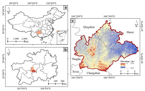
GNA is situated in the central region of Guizhou Province, with a spatial range of 26°11'7"N∼26°36'56"N, 105°56'20"E∼106°39'10"E, encompassing a planned area of 1795 km², with a core area of 470 km² (Figure 1). The terrain predominantly comprises low hilly landscapes, featuring higher elevations in the western part and lower elevations in the eastern portion, resulting in an overall gentle topography. The area experiences an average annual temperature ranging from 12.8 °C to 16.2 °C, with an average summer temperature of approximately 22.3 °C. GNA boasts an exceptional air quality rate of over 98% consistently over the years, and approximately 24% of the total area is covered by wetlands. In Guizhou Province, this location stands out for possessing highly favorable land conditions and relatively low development and construction costs. Ecotype land occupies approximately 88% of the total land resources in GNA, indicating a significant ecological role of land use and underscoring the challenging task of ecological environment protection in the area.

Figure 1. The situation of the study area.

(a. Location of Guizhou Province in China; b. Location of GNA in Guizhou; c. The core area of GNA)

2.2. Data source and processing

Image data are derived from the Landsat series of satellite images released by the United States Geological Survey (USGS). The spatial resolution is 30 m, and the Earth observation period is 16d. Using the Google Earth Engine platform, online access to the TM and OLI surface reflectance data products of the Landsat series in the research area is attained, and images of the vegetation growing season (5-10) are selected as reference images; moreover, the quality control band (QA) cloud mask algorithm is used for cloud processing. The selection of research time node takes into account the critical period of urban development in GNA. For example, infrastructure construction projects were launched in 2011, and it was officially established as a state-level new district in 2014. Accelerate the construction of sponge city in 2017, and further strengthen the construction of infrastructure and public service supporting facilities in Guian New Area in 2020. Meanwhile, due to the low latitude of the research area, satellite remote sensing is affected by large cloud and fog images, there are more data deletions, and there were problems such as missing strips in 2012. Combined with the development history of GNA, the average values of valid observations in the adjacent three-year growing season were synthesized to obtain images from 2010 (2009-2011), 2014 (2013-2015), 2017 (2016-2018), and 2020 (2019-2021). In order to avoid the interference of surface water on the indicators, the 30 m JRC annual water dataset (Pekel et al. 2016) on the GEE cloud platform was used for water masking. Finally, the spatial and temporal distribution map of RSEI in the target year of GNA of Guizhou Province was obtained. Other data are shown in Table 1, the population data was resampled to 30 m × 30 m.

Table 1. Data type and source.

Type	Name	Resolution	Source
LU/LC	CLCD	30 m	https://doi.org/10.5281/zenodo.4417810
Population	WorldPop	100 m	https://hub.worldpop.org/
DEM	SRTM	30 m	https://earthexplorer.usgs.gov

2.3. RSEI model

The EQ calculation adopts the principal component analysis method proposed by Xu in 2013. The normalized difference vegetation index (NDVI), wetness component of the tasseled cap transformation (TCT), the normalized difference impervious surface index (NDBSI), and the land surface temperature (LST) were used to characterize the remote sensing ecological index (RSEI) synthesized by the four ecological elements: greenness, wetness, dryness, and heat, respectively (Xu 2013). (1) $$\mathit{RSEI}=f\left(\mathit{WET},\mathit{NDVI},\mathit{LST},\mathit{NDBSI}\right)$$(1)

2.3.1. Greenness

Since the NDVI is closely related to plant biomass, leaf area index, and vegetation coverage (Zhong and Xu 2021), NDVI is used to characterize the greenness index of the research area. The expression is as follows: (2) $$\mathit{NDVI}=({\rho }_{\mathit{nir}}-{\rho }_{\mathit{red}})/({\rho }_{\mathit{nir}}+{\rho }_{\mathit{red}})$$(2) where ρ_nir and ρ_red represent the reflectance of the near-infrared and red bands of the remote sensing image, respectively.

2.3.2. Wetness

The moisture component based on the tasseled cap transformation can better reflect the wetness of surface water, soil, and vegetation, especially the moisture state of the soil (Baig et al. 2014). Due to the different band coefficients of different sensor images, the humidity index extraction formula is different when the humidity component is extracted by the satellite data of Landsat5 and 8. The calculation model is as follows: (3) $${\mathit{WET}}_{TM}=(0.0315{\rho }_{\mathit{blue}}+0.2021{\rho }_{\mathit{green}}+0.3102{\rho }_{\mathit{red}}+0.1594{\rho }_{\mathit{nir}}-0.6806{\rho }_{\mathit{swir}1}-0.6109{\rho }_{\mathit{swir}2})\times 0.0001$$(3) (4) $${\mathit{WET}}_{\mathit{OLI}}=(0.1511{\rho }_{\mathit{blue}}+0.1973{\rho }_{\mathit{green}}+0.3283{\rho }_{\mathit{red}}+0.3407{\rho }_{\mathit{nir}}-0.7171{\rho }_{\mathit{swir}1}-0.4559{\rho }_{\mathit{swir}2})\times 0.0001$$(4) where ρ_blue, ρ_green, ρ_red, ρ_nir, ρ_swir1, and ρ_swir2 represent the reflectivity of features in the blue, green, red, near-infrared, short-wave infrared band 1, and shortwave infrared band 2 of TM and OLI images, respectively.

2.3.3. Dryness

The construction and development of cities will inevitably replace the original natural ecosystem with man-made buildings, resulting in the "drying" of the surface. The dryness indicator is represented by the mean of the bare soil index (SI) (Rikimaru et al. 2002) and the index-based build-up index (IBI) (Xu 2008). The calculation formula is as follows: (5) $$\mathit{NDBSI}=(SI+\mathit{IBI})/2$$(5) (6) $$SI=\left[\left({\rho }_{\mathit{swir}1}+{\rho }_{\mathit{red}}\right)-\left({\rho }_{\mathit{blue}}+{\rho }_{\mathit{nir}}\right)\right]/\left[\left({\rho }_{\mathit{swir}1}+{\rho }_{\mathit{red}}\right)+\left({\rho }_{\mathit{blue}}+{\rho }_{\mathit{nir}}\right)\right]$$(6) (7) $$\mathit{IBI}=[2\times \frac{{\rho }_{\mathit{swir}1}}{{\rho }_{\mathit{swir}1}+{\rho }_{\mathit{nir}}}-(\frac{{\rho }_{\mathit{nir}}}{{\rho }_{\mathit{red}}+{\rho }_{\mathit{nir}}}+\frac{{\rho }_{\mathit{green}}}{{\rho }_{\mathit{swir}1}+{\rho }_{\mathit{green}}}\left)\right]/[2\times \frac{{\rho }_{\mathit{swir}1}}{{\rho }_{\mathit{swir}1}+{\rho }_{\mathit{nir}}}-(\frac{{\rho }_{\mathit{nir}}}{{\rho }_{\mathit{red}}+{\rho }_{\mathit{nir}}}+\frac{{\rho }_{\mathit{green}}}{{\rho }_{\mathit{swir}1}+{\rho }_{\mathit{green}}}\left)\right]$$(7) where ρ_green, ρ_blue, ρ_red, ρ_nir, ρ_swir1, and ρ_swir2 are the reflectance values of the green, blue, red, near-infrared, mid-infrared 1, and mid-infrared 2 bands of TM and OLI images, respectively.

2.3.4. Heat

LST is closely related to natural and human factors such as vegetation growth, urban water vapor cycle, urbanization process, etc. Therefore, surface temperature is used to represent heat indicators (Wang and He 2021). The heat index is expressed by inverting the surface temperature. Because band 10 in the two thermal infrared bands of Landsat8 has a higher atmospheric transmittance than band 11 (Wang et al. 2020), band6 of Landsat5 and band10 of Landsat8 are selected as the channels for LST inversion. The calculation formula is as follows: (8) $$L\lambda =\mathit{gain}\times DN+\mathit{bias}$$(8) (9) $$T=K2/\ln \hspace{0.17em}(K1/L\lambda +1)$$(9) where Lλ represents the radiation value of the pixels at the sensor of band 6 of the TM sensor and band 10 of the OLI sensor; DN is the gray value of the cell; gain and bias are the gain and bias values of the band6/10 band, respectively; T is the temperature value at the sensor; K1 and K2 are calibration parameters, obtained from the Landsat user manual and the latest revised calibration parameters surface temperature by Chander et al. (2009) The temperature T corrected by the specific emissivity can be converted to LST: (10) $$\mathit{LST}=T/[1+(\lambda T/\rho )\ln \hspace{0.17em}\epsilon$$(10) where λ is the center wavelength of TM, OLI band6, and band10: λ_TM=11.434 µm and λ_OLI=10.896 µm; ρ = 1.438 × 10-2mK; ε is the surface specific emissivity, the value of which is shown in Nichol (2005).

2.3.5. Integration of the four indicators

The NDVI, WET, LST, and NDBSI indicators are combined into comprehensive indicators via principal component transformation so that most information is concentrated in the first principal component (PC1) (Zheng et al. 2020). In order to avoid the influence of dimensional factors between different ecological factors, a single index is normalized. After normalization, the values of each indicator are unified within [0, 1], and the normalized calculation formula for each indicator is as follows: (11) $${NI}_i=(I_i-I_{\min })/(I_{\max }-I_{\min })$$(11) where NI_i is the normalized result of each indicator, I_i is the value of each indicator at cell i, and I_max and I_min are the maximum and minimum values of each indicator, respectively. Then, the principal component analysis method is used to generate RSEI₀ for the 4 component indexes after normalization. In order to facilitate the comparative analysis of the first principal component between different years, RSEI₀ is normalized, and finally RSEI is constructed: (12) $${\mathit{RSEI}}_0=PC1\left[f\right(\mathit{NDVI},\mathit{WET},\mathit{LST},\mathit{NDBSI}\left)\right]$$(12) (13) $$\mathit{RSEI}=({\mathit{RSEI}}_0-{\mathit{RSEI}}_{0\_\min })/\mathrm{ }({\mathit{RSEI}}_{0\_\max }-{\mathit{RSEI}}_{0\_\min })$$(13) where RSEI₀ is the un-normalized initial remote sensing ecological index, is the maximum value of ${\mathit{RSEI}}_{0\_\max }$RSEI₀, and is the minimum value of ${\mathit{RSEI}}_{0\_\min }$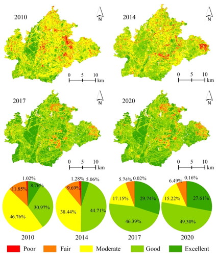RSEI₀. RSEI is the final remote sensing ecological index, and its value is within [0,1]. The closer it is to 1, the better the quality of the ecological environment. In order to further analyze the changes in the EQ in GNA, the RSEI values of each year in GNA were divided into five levels according to the equal interval division method (Figure 2), which represent poor (0-0.2), fair (0.2-0.4), moderate (0.4-0.6), good (0.6-0.8), and excellent (0.8-1) (Zhang et al. 2022a).

Figure 2. Spatial distribution and area ratio of RSEI from 2010 to 2020.

2.4. Spatial auto-correlation analysis

Spatial auto-correlation is an important indicator to test whether the attribute value of an element is correlated significantly with the attribute value of its adjacent space (Fan and Cowley 1985, Martin 1996). The spatial correlation analysis of EQ can be used to reveal the correlation of EQ between spatial units and their adjacent spatial units and describe the spatial uniformity of EQ (Zheng et al. 2021). In this paper, Moran’s I index (global spatial auto-correlation) and the local indicator of spatial association (LISA) are used to analyze the spatial correlation of EQ.

The global Moran’s I index is used to verify the spatial correlation of an element in the study area. The closer the absolute value of Moran’s I is to 1, the stronger the spatial autocorrelation. The calculation formula is as follows: (14) $${\mathit{Globalmoran}}^{’}s I=\frac{m\times {\sum }_{i=1}^m{\sum }_{j=1}^m{W}_{ij}(D_i-\overline{D})(D_j-\overline{D})}{{\sum }_{i=1}^m{\sum }_{j=1}^m{W_{ij}(D_i-\overline{D})}^2}$$(14) where m is the total number of indicators, D_i represents the EQ value of location i, is the average value of EQ of all indicators in the study area, $\overline{D}$W_ij is the spatial weight, and Moran’s I ranges within [-1,1]. The closer Moran’s I is to +1, the more pronounced the spatial positive autocorrelation of EQ; the closer Moran’s I is to −1, the greater the spatial difference in EQ, and 0 indicates that there is no spatial autocorrelation.

If global spatial autocorrelation does not exist, the LISA index (local spatial autocorrelation) can look for locations where local spatial autocorrelation may be masked. If global spatial autocorrelation exists, spatial heterogeneity can be analysed (Anselin 2010). The calculation formula is as follows: (15) $${\mathit{Localmoran}}^{’}s I=\frac{\left(D_i-\overline{D}\right)\times {\sum }_{j=1}^m{W}_{ij}(D_j-\overline{D})}{{\sum }_{i=1}^m{(D_i-\overline{D})}^2}$$(15) where Localmoran’s I represents the Local Moran’s I index, and the calculation parameters are the same as Moran’s I index. The LISA cluster map has 5 types of local spatial aggregation, namely High-High (HH), High-Low (HL), Low-Low (LL), Low-High (LH), and No Significant. In this study, HH/LL indicates a high/low EQ value of the selected region and spatially adjacent regions. HL indicates a high EQ value of the selected region but a low EQ value of the adjacent regions, and LH is the opposite.

2.5. Geodetector

Geodetector operate on the assumption that geographical objects always exist at specific spatial locations, and the environmental factors influencing their changes exhibit spatial variation. When there is a significant spatial consistency between an environmental factor and changes in geography, it plays a crucial role in the occurrence and development of geographical objects (Wang et al. 2010). Geodetector, as a spatial statistics method, serves the purpose of analyzing geographic heterogeneity and quantifying the impact of drivers (Zhang et al. 2022a). The Geodetector consists of four parts:

(1) The factor detector, which assesses the spatial heterogeneity of RSEI and the extent to which various factors influence RSEI. The calculation formula is as follows: (16) $$q=1-\frac{1}{{N\sigma }^2}{\sum }_{h=1}^L{N_h\sigma }_h^2$$(16) where the q value measures the explanatory power of each factor on RSEI and ranges from 0 to 1. A higher q value indicates a stronger explanatory influence of the factor on RSEI. L represents the number of categories in RSEI; N_h and N represent the number of RSEI units in layer h and the entire area, respectively. and ${\sigma }_h^2$σ² represent the variance of RSEI values in layer h and the entire area, respectively.

(2) The interaction detector serves the purpose of identifying the interplay between impact factors (Peng et al. 2019), specifically detecting how two different impact factors jointly influence RSEI. The types of interactions can be divided into the Nonlinear enhancement, Single factor nonlinearity attenuation, Two-factor enhancement, Independent, Nonlinear attenuation.

(3) The ecological detector aims to compare the spatial distribution of RSEI between the two impact factors and determine if there are significant differences, which is quantified using the F statistic. The formula for the F statistic is as follows: (17) $$F=\frac{N_{X_1}(N_{X_2}-1){\sum }_{h=1}^{L_1}{N_h\sigma }_h^2}{N_{X_2}(N_{X_1}-1){\sum }_{h=1}^{L_2}{N_h\sigma }_h^2}$$(17)

Where and represent the number of samples for impact factors and respectively. The other variables remain the same as those in the factor detector.${\mathrm{N}}_{{\mathrm{X}}_1}$${\mathrm{N}}_{{\mathrm{X}}_1}$${\mathrm{X}}_1\mathrm{ }$${\mathrm{X}}_2,$

(4) The risk detector is employed to assess whether there are significant differences in the mean of the dependent variable among subregions. Specifically, it helps identify areas where RSEI either degrades or improves. The detector uses t to test this: (18) $$t=\frac{{\overline{Y}}_{H=1}-{\overline{Y}}_{h=2}}{{[\frac{\mathit{Var}\left(Y_{h=1}\right)}{n_h=1}+\frac{\mathit{Var}\left(Y_{h=2}\right)}{n_h=2}]}^{\frac{1}{2}}}$$(18)

Where, represents the mean of the RSEI linear regression coefficient in subregion h; is the number of samples in subregion h; Var denotes variance.$\overline{Y}$$n_h$

Based on prior research (Xia et al. 2022, Wang et al. 2023, Yi et al. 2023) and the specific conditions of GNA, considering data availability, four external factors (LU/LC, population, elevation, slope) and four model factors (NDVI, WET, LST, NDBSI) were selected as the influencing factors for EQ detection and quantitative attribution analysis.

3. Results

3.1. RSEI model inspection

The principal component analysis method was used to obtain the results of the four indicators of greenness, humidity, heat, and dryness (Table 2). As observed in the table, the contribution rate of PC1 in 2010, 2014, 2017, and 2020 was 71.33%, 77.80%, 81.98%, and 82.75%, indicating that the first principal component has concentrated most of the characteristic information of the four component indicators. In the PC1 of each year, the NDVI and WET feature vectors that have positive ecological significance are both positive, and the NDBSI and LST feature vectors that have negative ecological significance are both negative, indicating that PC1 has ecological significance for ecological environment evaluation.

Table 2. PCA results of RSEI from 2010 to 2020.

Indicators	2010	2014	2017	2020
NDVI	0.70	0.73	0.78	0.82
WET	0.08	0.17	0.12	0.11
NDBSI	−0.52	−0.62	−0.56	−0.50
LST	−0.49	−0.23	−0.25	−0.26
Eigenvalue	0.03	0.04	0.05	0.04
Percent eigenvalue	71.33%	77.80%	81.98%	82.75%

The mean RSEI of each year calculated by the ecological index is shown in Table 2. In general, the RSEI value of GNA showed a trend that first increased and then declined. It rose from 0.57 in 2010 to a maximum value of 0.70 in 2017 and then fell to 0.69 in 2020, indicating that the EQ of GNA has shown a trend of improvement in the past 10 years. Comparing the annual changes of the four indicators, the mean greenness indicators were 0.48, 0.60, 0.62, and 0.65, respectively, which showed a straight upward trend from 2010 to 2020, while the humidity indicators showed a fluctuating downward trend, but they all exceeded 0.8. Both the dryness index and the heat index showed a fluctuating trend that increased first, decreased, and then increased again. By 2020, the dryness index increased by a total of 0.7, and the heat index was the same as in 2010. In general, the negative effect of the dryness and heat index on the EQ of GNA is lower than the positive effect of the greenness index and humidity index, which is consistent with the results of RSEI (Table 3).

Table 3. Remote sensing ecological indicators and RSEI mean statistics

Year	Indicators				RSEI
	NDVI	WET	NDBSI	LST
2010	0.48	0.92	0.38	0.42	0.57
2014	0.60	0.83	0.50	0.56	0.59
2017	0.62	0.80	0.41	0.39	0.70
2020	0.65	0.85	0.45	0.42	0.69

3.2. Analysis of spatiotemporal changes in EQ

3.2.1. Spatial and temporal distribution pattern of EQ

Conduct spatial distribution and area comparison of EQ at different levels in the research area, and quantitatively analyze the s temporal and spatial changes of EQ in GNA from 2010 to 2020. As observed in Figure 2, the areas with medium EQ in 2010 were widely distributed within the scope of the research area, accounting for 46.76% of the research area. In 2014, the area with good EQ increased significantly, and the distribution area was wider, accounting for 44.71%. The area with medium EQ decreased by 8.32%, and the area of poor and fair areas decreased by a total of 1.90%. The spatial distribution pattern also showed a large difference, because after the establishment of GNA was officially approved, the construction of roads and buildings began, resulting in poor EQ and fair areas that are mainly distributed in roads and urban construction areas in the central and eastern parts in strips and groups. In 2017, with the exception of some areas in the north, the middle, and the east, most of the areas were in a good ecological state, and the southern regions were mostly ecologically excellent. The total area of the area with good and excellent ecology was 357.81 km², accounting for 76.13% of the total area of the study area, and environmental degradation near the road and urban area was significantly improved, which was manifested as medium EQ; thus, the area of poor and poor EQ decreased significantly, exhibiting a total decrease of 5.21%. By 2020, due to urban development, the area that exhibited poor and fair grades tended to increase outward and inward, and the total area increased by 0.89%, but the overall distribution pattern of EQ was basically unchanged from that of 2017.

Overall, from 2010 to 2020, the EQ of GNA was mainly good. With the exception of 2010, when the EQ accounted for the largest proportion of medium grade, the other years exhibited the largest proportion of good grade, and all of them exceeded 45%; moreover, the proportion of area accounted for by the sum of poor and poor decreased by 6.22% overall, and the overall ecological environment was greatly improved. Spatially, RSEI high-quality areas are mainly distributed in mountainous areas in the central and southern regions, and low-value areas are mainly distributed in urban construction areas, indicating that the ecological environment quality of GNA is mainly affected by topography and urban expansion. In addition, we also observed that there are also high-value EQ areas in areas that are low, indicating that while land construction and road expansion take place, green belts, green spaces, and other land are also added, causing the phenomenon of "urban greening" and offsetting the impact of urbanization on the regional EQ.

3.2.2. Changes in EQ transfer

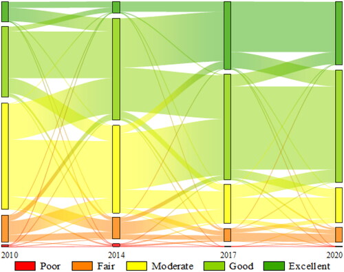
In order to observe the EQ transfer of each ecological grade in GNA from 2010 to 2020, the Sankey diagram was used to express the detailed EQ change process of GNA from 2010 to 2020 (Figure 3). Throughout the research period, the EQ was mainly at a moderate or good level. Specifically, from 2010 to 2017, EQ showed an upward trend: the area exhibiting moderate, fair, and poor levels decreased, areas exhibiting excellent and good levels increased significantly, and the EQ level changed from moderate, good, poor, and excellent to good, excellent, and moderate, respectively. During the period from 2017 to 2020, the EQ did not decrease significantly, mainly manifested at the excellent level of EQ, and the area exhibiting good inflow is 2% larger than the area exhibiting good to excellent levels.

Figure 3. The transition matrix of different EQ levels from 2010 to 2020.

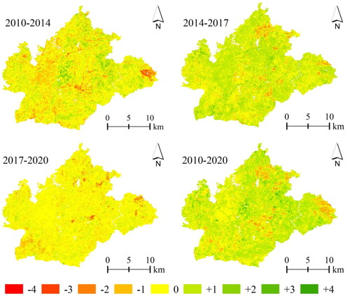
By utilizing the principle of difference, we examined the temporal and spatial changes in EQ during various periods from 2010 to 2020, based on the EQ Sankey diagram shown in Figure 3 (Figure 4). The changes were categorized into different levels: +4, +3, +2, and +1 denoting improvement; 0 indicating no change; and −1, −2, −3, and −4 indicating degradation, with larger values indicating more significant changes. From 2010 to 2014, the changes in EQ were primarily concentrated between +1 and −1, with level 0 accounting for over 50% of the area, and the area of level +1 being 6.50% more than that of level −1. The areas with improved EQ were “large dispersion and small aggregation,” while degraded areas tended to be distributed in strips or clusters, coinciding with the road and urbanization planning in the region. This period mainly witnessed grade −4 changes, albeit not exceeding 0.01% of the total area, which could be attributed to the implementation of “road greenways” in GNA. During 2014-2017, the main period of EQ improvement, 59.48% of the area experienced enhanced EQ, with level +1 changes being most significant, accounting for 89.87% of the improved area. Ecological degradation was observed in only 6.55% of the total research area, with levels +4, −3, and −4 being practically absent, reflecting GNA’s efforts in ecological governance. From 2017 to 2020, EQ displayed a declining trend, with the area experiencing degradation being slightly larger than that showing improvement. However, areas with unchanged quality dominated, accounting for 72.67% and widely distributed across the study area. Overall, the changes in EQ in GNA over the past decade predominantly occurred between adjacent levels (+1 and 0), constituting 46.07% and 32.77% of the change area, respectively. Changes at levels ±3 and +4 were minimal, with the overall change area being less than 0.05%, indicating that the ecological quality changes mainly occurred within neighboring levels and exhibited less pronounced regional evolution across different EQ levels.

Figure 4. RSEI Detection change from 2010 to 2020.

3.3. The response of EQ to changes in land cover

The change in land cover type will cause a transformation in the material and energy cycle within the region, which will have a significant impact on regional EQ and produce obvious ecological environmental effects (Wang et al. 2019b). Therefore, the types of land cover in 2010, 2014, 2017, and 2020 were obtained, and the relationship between the EQ and land cover in the research area was investigated based on RSEI results.

By spatially superimposing the types of land cover in each time period of the research area, a Sankey diagram of the conversion of land cover types from 2010 to 2020 is obtained. As observed in Figure 5, the cropland and forest in the research area occupied a dominant position in all four periods, and the bare soil covered the smallest area. Specifically, from 2010 to 2020, cropland showed a decreasing trend, with a total decrease of 2.82%, but it still maintained a dominant position. In addition to the transfer of cropland to its own type, cropland mainly transferred to forest and grassland, which was the most transferred from 2014 to 2017 with a total of 19.77 km², and this was mainly due to the return of farmland to forest and grassland, and the corresponding forest and grassland area showed an increasing trend. Not only is the amount of transfer of water bodies, bare soil, and impermeable surfaces small and the type of transfer is relatively singular, but the impermeable surface flows in most areas and does not flow out, and the inflow area shows a linear growth trend, reflecting that the great changes were introduced to the ecological pattern of the GNA during the 10 years of urban construction in the study area.

Figure 5. The transition matrix of different LU/LC from 2010 to 2020.

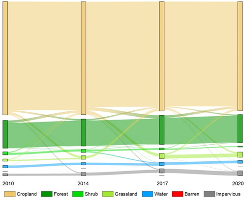
From the perspective of various time periods, the land cover situation changed the most from 2014 to 2017, followed by 2017–2020. Because the concept of GNA was first proposed in 2011, it was officially approved as a new national area in 2014; in the early stage of development, GNA mainly focused on infrastructure construction and established preliminary urban functions within two or three years, and after 2017, the development momentum slowed down. The land cover change in GNA is basically consistent with its urbanization development process.

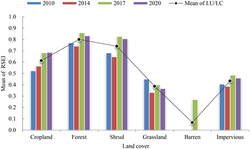
Calculate the RSEI average for different land cover types (Figure 6). It was found that the mean RSEI of various LU/LC types is forest (0.80), shrub (0.74), cropland (0.61), impervious (0.43), grassland (0.39), barren (0.07) from high to low. From 2010 to 2020, the RSEI for barren only showed 0.27 in 2017, and 0 in the rest of the years. The accuracy of data can influence the spatial representation and area calculations of bare ground, potentially resulting in errors in the expression of bare ground within RSEI. Human activities have a large impact on the EQ of grassland and have a negative impact, and its RSEI has shown an overall downward trend, with the largest decline in the period 2010–2014. The EQ of various other types has increased to varying degrees. And the mean RSEI of cultivated land and shrubs has increased the most, by 0.16 and 0.06, respectively, indicating that RSEI is mainly increased in the form of cropland and shrubs. The average RSEI of the impervious surface showed an overall upward trend. The most prominent period is 2014–2017, when the quality of the ecological environment rose from 0.39 to 0.48, indicating that “urban greening” has effectively improved the EQ of urban construction areas.

Figure 6. RSEI average by LU/LC from 2010 to 2020.

3.4. Spatial auto-correlation analysis of EQ

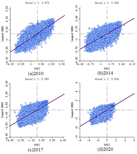
In order to explore the RSEI spatial autocorrelation in GNA from 2010 to 2020, the RSEI images of 2010, 2014, 2017, and 2020 were resampled to a scale of 100 m × 100 m, and a total of 49140 sample points were collected to determine the spatial correlation of variables and their correlation; then, Moran’s I index was used to analyze global autocorrelation, and the LISA plot was used to analyze local autocorrelations. Figure 7 shows the Moran’s I index scatter plots of GNA in 2010, 2014, 2017, and 2020, which are mainly distributed in the first and third quadrants, indicating that there is a strong spatial positive correlation between EQ in the study area. In 2010, 2014, 2017, and 2020, the values of Moran’s I were 0.678, 0.568, 0.590, and 0.604, respectively, showing a downward and then upward trend, indicating that the spatial distribution of ecological environment quality in the research area is aggregated and not random, and the agglomeration shows a trend that weakens first and then increases. After 2014, the urbanization process accelerated, resulting in the dispersion of high-ecological-quality areas in the region. With the completion of urban construction areas, various EQ points merged into plaques, and homogeneity increased.

Figure 7. Scatterplot of RSEI Moran’s I from 2010 to 2020.

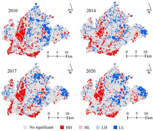
The LISA cluster diagram can be used to better understand the spatial EQ of RSEI characteristics (Saleh et al. 2021). As shown in Figure 8, the overall EQ of GNA from 2010 to 2020 is mainly based on the HH agglomeration area and the LL agglomeration area, and there are fewer “qualitative differences” in the HL or LH space. HH agglomeration areas are mainly distributed in mountainous areas with high vegetation coverage in the central and western regions and the south; LL agglomeration areas are mainly distributed in urbanized development zones in the north, central, and eastern regions, with large population activities, such as Huaxi University City in the east. In 2014, the LL agglomeration area also showed grid-like characteristics due to road construction, and then this characteristic disappeared, indicating that the ecological measures of road greening have a positive effect on the quality of the ecological environment. The LH agglomeration area is mainly distributed in and around the mountains and then spreads to the surrounding urban development zones. While destroying the original ecology, humans have also strengthened ecological construction. HL agglomeration areas are mainly distributed in or around urban construction areas, indicating that although vegetation is directly affected and reduced in urban construction, vegetation growth in cities is increasing; that is, there are extensively positive indirect effects from the urban environment on vegetation growth, which indicates that ecological construction has significant effects in the process of urbanization. In general, the spatial agglomeration characteristics of EQ in GNA are affected by topography and geomorphology, socio-economic development, and ecological construction, and their variation characteristics are consistent with the temporal and spatial changes in RSEI in the study area.

Figure 8. LISA of the RSEI from 2010 to 2020.

3.5. Analysis of the driving factors of RSEI temporal and spatial changes

3.5.1. Single factor assay analysis

Table 4 presents compelling evidence that all eight factors significantly influence changes in RSEI (p < 0.001). Among these factors, land cover, altitude, slope, and population demonstrate varying degrees of influence on RSEI from 2010 to 2020. Notably, land cover emerges as the most crucial factor, with its explanatory power on the rise. Conversely, the explanatory power of population, altitude, and slope shows a decline to varying extents. This trend indicates that the rapid development of the social economy, which drives changes in land cover types by humans, has strengthened its impact on EQ and emerged as a key factor affecting RSEI. Focusing on the model factors, NDVI and NDBSI exhibit higher explanatory power for RSEI compared to WET and LST. This finding underscores that the changes in EQ within GNA from 2010 to 2020 are primarily influenced by the increase in vegetation coverage and the expansion of impermeable surfaces. These factors contribute to the decline of GNA’s EQ from 0.70 to 0.69 during the later period.

Table 4. Analysis of factors affecting RSEI from 2010 to 2020.

Year	Factors	External factors				Model factor
		LU/LC	Population	Elevation	Slope	NDVI	WET	LST	NDBSI
2010	q	0.4062	0.0907	0.2095	0.1309	0.7923	0.5018	0.5112	0.7947
	p	0.000	0.000	0.000	0.000	0.000	0.000	0.000	0.000
2014	q	0.3341	0.0695	0.1084	0.0715	0.8868	0.5860	0.2606	0.8922
	p	0.000	0.000	0.000	0.000	0.000	0.000	0.000	0.000
2017	q	0.4216	0.0601	0.1364	0.1036	0.9223	0.5558	0.3405	0.8876
	p	0.000	0.000	0.000	0.000	0.000	0.000	0.000	0.000
2020	q	0.4333	0.0509	0.1201	0.0823	0.9288	0.6082	0.4211	0.8908
	p	0.000	0.000	0.000	0.000	0.000	0.000	0.000	0.000

3.5.2. Interaction detector and ecological detector

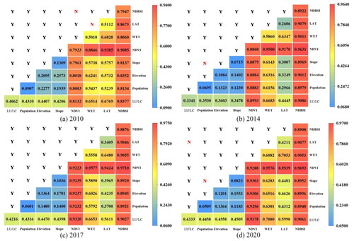
Using the Geodetector approach, we employed the interaction detector and ecological detector to investigate the factors influencing RSEI in GNA. The results were obtained with a 95% confidence level. Figure 9 illustrates the spatial variations in RSEI within the study area, which were consistently marked by two-factor enhancement when any two factors interacted. This suggests that the spatial differentiation of EQ in GNA results from the combined effects of various influencing factors. The synergy between NDVI and NDBSI, along with other driving factors, exhibited a high interaction explanatory force, with a q value above 0.79. Among the external factors, LU/LC and other drivers demonstrated the strongest explanatory power, with a q value exceeding 0.34. Notably, in the univariate detection, the population’s q value was below 0.1, indicating limited individual explanatory power. However, when interacting with other factors like LC, the influence of population on the spatial differentiation characteristics of RSEI became more pronounced. Moreover, during ecological detection, we found that the interactions between NDVI and NDBSI, WET and LAT in 2010, as well as Population and Slope in 2014, and LC and LAT, Population and Slope in 2020, were all assessed as non-significant (N). This implies that the collective impact of these detection factors on the spatial variations of RSEI does not show any significant differences. Overall, the development and construction activities in GNA led to substantial surface landscape transformations. These transformations had considerable effects on vegetation distribution and human activity areas, which, in turn, influenced various factors and ultimately manifested in changes in EQ.

Figure 9. 2010–2020 RSEI interaction detector and ecological detector matrix.(Y is significant and N is non-significant).

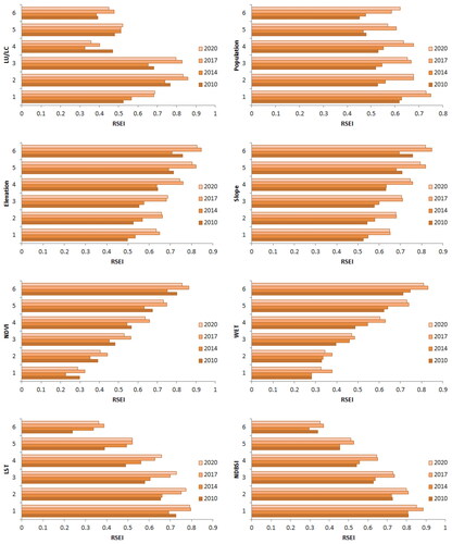
3.5.3. Risk detector

Using the risk detector, we identified the favorable range and types of factors affecting RSEI (Regional Ecological Security Index). Each impact factor was categorized into six levels, represented by numbers 1 to 6, and all of them passed the statistical test at a 95% confidence level (Figure 10). Specifically, the LU/LC levels 2 and 3, characterized by forests and shrubs, consistently exhibited higher RSEI values in different years, indicating that these were the most beneficial LU/LC types for promoting RSEI. Regarding population factors, there was a general trend of decreasing RSEI with increasing population each year. However, it’s worth noting that at the same level of population, the RSEI value in 2020 was higher than that in 2010. This finding indirectly suggests that human activities might have a positive effect on EQ. Both altitude and slope displayed a positive correlation with RSEI, indicating that higher altitudes and steeper slopes were associated with lower ecological pressure. Among the model factors, NDVI and WET exhibited a positive feedback effect on EQ, meaning that higher values of these factors were conducive to better ecological conditions. Conversely, LST and NDBSI showed the opposite effect, where higher values of these factors were linked to decreased EQ.

Figure 10. Statistical results of RSEI at different levels of influence factors.

4. Discussion

4.1. The impact of urbanization on EQ

The rapid urbanization has led to the conversion of numerous rural and suburban regions into urban areas, driving regional development and causing significant changes in LU/LC, becoming a crucial factor affecting the alteration of regional EQ (Hu et al. 2023). Numerous studies have highlighted the substantial impact of LU/LC changes on urban ecosystems, with large-scale urban development and construction frequently resulting in declining EQ in the affected regions (Deng et al. 2023). Particularly in the early stages of urbanization, the enhancement of EQ is constrained, leading to adverse effects on the overall environment (Hang et al. 2020). Shi et al. (2019) conducted an evaluation of EQ changes in the Gui’an Development Zone, situated in the Aojiang River Basin of Fujian Province. They deduced that the expansion of construction land significantly diminishes the quality of the regional ecological environment, with the RSEI value declining by 0.041 for every 10% increase in the proportion of construction land. Similarly, Cui et al. (2022b) assessed the EQ of Huaibei City and observed that urban construction encroached upon various land types, directly contributing to the decline in EQ. In our study focused on the urbanization process in GNA, we found that the RSEI increased from 0.57 to 0.69, despite the presence of urban construction areas experiencing deteriorating ecological conditions. This improvement can be attributed to two primary reasons. Firstly, urbanization prompts the migration of rural populations to urban centers, resulting in a decline in EQ in the urban and surrounding areas. Simultaneously, ecological initiatives, such as converting idle farmland back to forests and grasslands, have been implemented, leading to increased forest and grassland areas and improved vegetation coverage. Secondly, GNA holds the distinctive role of being the country’s sole new area with a primary focus on constructing ecological civilization. This responsibility entails the strategic goal of green development. Throughout the development process, efforts have been made to advance the establishment of ecological civilization demonstration zones and sponge cities. Comprehensive management and protection measures have been introduced for mountains, rivers, forests, fields, and lakes. Furthermore, a network of urban road greenways covering a total of 212 km has been built, culminating in a landscape system of “city in the forest and forest in the city”. This outcome serves as an exemplar of successful ecological preservation in the face of rapid urbanization for other ecologically fragile regions.

This study yields a significant revelation: urbanization is no longer an exclusively unidirectional influence on EQ. In the case of karst mountain cities like GNA, both stringent ecological protection measures and well-planned construction play pivotal roles in preserving and enhancing EQ. Nevertheless, it is noteworthy that the RSEI of GNA exhibited a decline of 0.1 after 2020, indicating that urbanization’s impact on EQ is not always beneficial. A study conducted by Li et al. (2023) on the coupling and coordination of urbanization and the ecological environment in Aba Prefecture, Sichuan Province, revealed that urbanization initially aids in reducing the overall pressure of human activities and improving EQ. However, as urbanization progresses, its positive effect on EQ diminishes due to an increase in resource and energy consumption. As a result, GNA must continue to bolster the protection and restoration of ecosystems and ecologically fragile regions, alongside devising sound urban planning to prevent further degradation of EQ and enhance urbanization coordination. In essence, it is crucial to conduct further analyses on the coupling relationship between urbanization and EQ, serving as the next step in research. By doing so, this effort will furnish a more reasoned theoretical and decision-making foundation for GNA to achieve sustainable and coordinated development amid the process of economic integration and the development of new urbanization.

4.2. Driving factors of the spatio-temporal variation of EQ

The findings reveal that the spatial differentiation of EQ within the study area is influenced by the complex interactions among multiple factors. Notably, NDVI and NDBSI from the model factors, along with LU/LC from external factors, emerge as the primary influencing factors and key drivers of regional EQ. Additionally, while the population alone exhibits a relatively lower explanatory power on EQ, its impact gains significance when interacting with other factors, such as LU/LC. In risk detection, despite the negative effect of population on EQ, the RSEI value in 2020 surpasses that of 2010 at the same level. This observation suggests that population does not directly influence EQ but rather indirectly affects it by altering the patterns of LU/LC. As a result, for future ecological planning and management in GNA, it is crucial to strengthen the positive role of human intervention in EQ. This entails scientifically transforming the mode of LU/LC, optimizing the urban spatial pattern, and ensuring the sustainable and favorable development of urban EQ.

4.3. Limitations and deficiencies

The mountainous area of the Guizhou Plateau has cloudy and rainy weather, and the cloud cover observed in optical satellite image data is large, making it one of the provinces with the least effective data (ground images without cloud and fog) obtained by optical satellite remote sensing in China (Huang et al. 2021a). Using the powerful cloud computing capability provided by GEE, the cloud-free images of the vegetation growing season in the three years before and after the target year were obtained by superimposing and extracting the median value. Then, based on the RSEI model, the EQ of GNA from 2010 to 2020 was evaluated and monitored. This avoids the influence of human factors to a large extent, comprehensively and objectively reflects the spatial distribution pattern and evolution trend of EQ in the past 10 years before and after the construction of GNA, and verifies the ecological construction effect of GNA in the process of urban development; all these provide a theoretical basis for the next stage of EQ protection and the sustainable development of GNA.

Although our method has shown some effectiveness in EQ evaluation against historical spatiotemporal changes, the limitations of this method will be further explored in future studies. First of all, our data comprise information from image synthesis that took place three years before and after, which solves the problem of missing images in cloudy and rainy areas, but this is not conducive to long-term continuous monitoring in a year-by-year or month-by-month manner. Future research will use cloudless image splicing or multi-source remote sensing fusion to complete the monitoring of EQ. Secondly, despite the CLCD dataset having an overall accuracy of 80%, the karst zone exhibits substantial surface heterogeneity and fragmentation characteristics. Consequently, optical remote sensing images in this region suffer from geometric and spectral distortions, leading to inaccuracies in the LU/LC products’ overall accuracy. Future research will use higher-precision land cover data to analyze EQ, which will be more conducive to decision makers to optimize the relationship between economic development and environmental protection.

5. Conclusions

This study presents a quantitative analysis of the spatio-temporal change pattern of EQ (EQ) in GNA, a nationally designated new area in China, over the period from 2010 to 2020, considering the context of rapid urbanization. Additionally, the Geodetector approach is employed to assess the explanatory influence of model factors and external factors on the spatial differentiation characteristics of RSEI. The key findings are summarized as follows:

1. During the period from 2010 to 2020, GNA exhibited a favorable trend in EQ, as evidenced by the increase in RSEI from 0.57 to 0.69. The analysis of RSEI level changes revealed that the significant variations (±3, +4) accounted for less than 5% of the total change area, while the majority of EQ changes were concentrated between +1 and 0.

2. EQ in GNA displayed spatial autocorrelation, with mountainous regions experiencing relatively stable EQ, consistent with the distribution of EQ HH agglomeration areas. On the other hand, areas showing EQ degradation and LL agglomeration were predominantly located in urban construction zones. Local governments should comprehensively consider the spatial heterogeneity of EQ, make overall planning and reasonable arrangements in advance, and ensure that EQ remains stable or continues to rise.

3. The LU/LC transfer analysis indicated that forest and impervious witnessed the largest inflow, with forest having the highest RSEI value (0.80) and barren the lowest (0.07). Except for grassland and barren, the mean RSEI value for other LU/L types exhibited varying degrees of increase.

4. Employing the geographic detector, the analysis identified NDVI from the model factors and LU/LC factors from the external factors as the primary driving forces influencing EQ in GNA. In the future, vegetation protection and urban greening projects should be strengthened to improve ecological quality.

Author contributions

Data curation, F.Z., S.D.; writing—original draft preparation, F.Z.; writing—review and editing, Z.Z., D.H, X.D., F.D. and Y.Y.; supervision, Z.Z.; project administration, F.Z.; funding acquisition, F.Z. All authors have read and agreed to the published version of the manuscript.

Disclosure statement

No potential conflict of interest was reported by the authors.

Data availability statement

The authors confirm that the data supporting the findings of this study are available within the article.

Additional information

Funding

This research was funded by the National Natural Science Foundation of China (41661088), and the Guizhou Province High-level Innovative Talent Training Plan “Hundred” Level Talents (Qiankehe Platform Talents [2016]5674).

References

- Aizizi Y, Kasimu A, Liang HW, Zhang XL, Zhao YY, Wei BH. 2023. Evaluation of ecological space and ecological quality changes in urban agglomeration on the northern slope of the Tianshan mountains. Ecol Indic. 146(17):109896. doi: 10.1016/j.ecolind.2023.109896.
- Anselin L. 2010. Local indicators of spatial association—Lisa. Geogr Anal. 27(2):93–115. doi: 10.1111/j.1538-4632.1995.tb00338.x.
- Baig MHA, Zhang L, Shuai T, Tong Q. 2014. Derivation of a tasselled cap transformation based on landsat 8 at-satellite reflectance. Remote Sens Lett. 5(5):423–431. doi: 10.1080/2150704X.2014.915434.
- Chander G, Markham BL, Helder DL. 2009. Summary of current radiometric calibration coefficients for landsat MSS, TM, ETM+, and EO-1 ALI sensors. Remote Sens Environ. 113(5):893–903. doi: 10.1016/j.rse.2009.01.007.
- Chen W, Huang H, Tian Y, Du Y. 2019. Monitoring and assessment of the eco-environment quality in the Sanjiangyuan region based on google earth engine. J Geo-Information Sci. 21(9):1382–1391. doi: 10.12082/dqxxkx.2019.190095.
- Chen W, Wang J, Ding J, Ge X, Han L, Qin S. 2023. Detecting long-term series eco-environmental quality changes and driving factors using the remote sensing ecological index with salinity adaptability (rseisi): a case study in the Tarim River Basin, China. Land. 12(7):1309. doi: 10.3390/land12071309.
- Cui J, Zhu M, Liang Y, Qin G, Li J, Liu Y. 2022a. Land use/land cover change and their driving factors in the yellow river basin of Shandong province based on google earth engine from 2000 to 2020. IJGI. 11(3):163. doi: 10.3390/ijgi11030163.
- Cui R, Han J, Hu Z. 2022b. Assessment of spatial temporal changes of ecological environment quality: a case study in Huaibei City, China. Land. 11(6):944. doi: 10.3390/land11060944.
- Deng W, Wen X, Xu H, Duan W, Li C. 2023. Analysis of regional development and its ecological effects: a case study of the Xiong′an New Area, China. Acta Ecol Sin. 1:263–273. doi: 10.5846/stxb202111233303.
- Fan GY, Cowley JM. 1985. Auto-correlation analysis of high resolution electron micrographs of near-amorphous thin films. Ultramicroscopy. 17(4):345–355. doi: 10.1016/0304-3991(85)90201-3.
- Geng R, Yin P, Ma Q. 2018. Simulation research for ecological security pattern construction based on improvement of water and air quality in GNA. China Environ Sci. 5:1990–2000. doi: 10.19674/j.cnki.issn1000-6923.2018.0221.
- Hang X, Li Y, Luo X, Xu M, Han X. 2020. Assessing the ecological quality of Nanjing during its urbanization process by using satellite, meteorological, and socioeconomic data. J Meteorol Res. 34(2):280–293. doi: 10.1007/s13351-020-9150-6.
- He Y, You N, Cui Y, Xiao T, Hao Y, Dong J. 2021. Spatio-temporal changes in remote sensing-based ecological index in China since 2000. J Nat Resour. 36(5):1176. doi: 10.31497/zrzyxb.20210507.
- Hu C, Song M, Zhang A. 2023. Dynamics of the eco-environmental quality in response to land use changes in rapidly urbanizing areas: a case study of Wuhan, China from 2000 to 2018. J Geogr Sci. 33(2):245–265. doi: 10.1007/s11442-023-2081-2.
- Huang D, Zhou Z, Peng R, Zhu M, Yin L, Zhang Y, Xiao D, Li Q, Hu L, Huang Y. 2021a. Challenges and main research advances of low-altitude remote sensing for crops in southwest plateau mountains. J Guizhou Norm Univ. 5:51–59. doi: 10.16614/j.gznuj.zrb.2021.05.008.
- Huang H, Chen W, Zhang Y, Qiao L, Du Y. 2021b. Analysis of ecological quality in Lhasa metropolitan area during 1990–2017 based on remote sensing and google earth engine platform. J Geogr Sci. 31(2):265–280. doi: 10.1007/s11442-021-1846-8.
- Ji J, Wang S, Zhou Y, Liu W, Wang L. 2020a. Spatiotemporal change and landscape pattern variation of eco-environmental quality in Jing-Jin-Ji urban agglomeration from 2001 to 2015. IEEE Access. 8:125534–125548. doi: 10.1109/ACCESS.2020.3007786.
- Ji JW, Wang SX, Zhou Y, Liu WL, Wang LT. 2020b. Studying the eco-environmental quality variations of jing-jin-ji urban agglomeration and its driving factors in different ecosystem service regions from 2001 to 2015. IEEE Access. 8:154940–154952. doi: 10.1109/ACCESS.2020.3018730.
- Jing Y, Zhang F, He Y, Kung H-T, Johnson VC, Arikena M. 2020. Assessment of spatial and temporal variation of ecological environment quality in ebinur lake wetland national nature reserve, Xinjiang, China. Ecol Indic. 110:105874. doi: 10.1016/j.ecolind.2019.105874.
- Li J, Knapp DE, Lyons M, Roelfsema C, Phinn S, Schill SR, Asner GP. 2021. Automated global shallow water bathymetry mapping using google earth engine. Remote Sens. 13(8):1469. doi: 10.3390/rs13081469.
- Li YK, Li XZ, Lu T. 2023. Coupled coordination analysis between urbanization and eco-environment in ecologically fragile areas: a case study of northwestern Sichuan, Southwest China. Remote Sens. 15(6):1661. doi: 10.3390/rs15061661.
- Liu MX, Ma MF, Liu JH, Lu XQ, Dong ZY, Li JN. 2023. Quantifying impacts of natural and anthropogenic factors on urban ecological quality changes: a multiscale survey in Xi’an, China. Ecol Indic. 1539(14):10463. doi: 10.1016/j.ecolind.2023.110463.
- Liu TL, Ren C, Zhang SG, Yin AC, Yue WT. 2022. Coupling coordination analysis of urban development and ecological environment in urban area of Guilin based on multi-source data. Int J Env Res Pub He. 19(19):12583. doi: 10.3390/ijerph191912583.
- Liu Y, Wang J. 2022. Revealing annual crop type distribution and spatiotemporal changes in northeast china based on google earth engine. Remote Sens. 14(16):4056. doi: 10.3390/rs14164056.
- Liu Y, Wang Y, Peng J, Du Y, Liu X, Li S, Zhang D. 2015. Correlations between urbanization and vegetation degradation across the world’s metropolises using DMSP/OLS nighttime light data. Remote Sens. 7(2):2067–2088. doi: 10.3390/rs70202067.
- Martin D. 1996. An assessment of surface and zonal models of population. Int J Geogr Inf Syst. 10(8):973–989. doi: 10.1080/02693799608902120.
- Najafzadeh F, Mohammadzadeh A, Ghorbanian A, Jamali S. 2021. Spatial and temporal analysis of surface urban heat island and thermal comfort using landsat satellite images between 1989 and 2019: a case study in Tehran. Remote Sens. 13(21):4469. doi: 10.3390/rs13214469.
- Nichol J. 2005. Remote sensing of urban heat islands by day and night. Photogramm Eng Remote Sensing. 71(5):613–621. doi: 10.14358/PERS.71.5.613.
- Pekel JF, Cottam A, Gorelick N, Belward AS. 2016. High-resolution mapping of global surface water and its long-term changes. Nature. 540(7633):418–422. doi: 10.1038/nature20584.
- Peng W, Zhang D, Luo Y, Tao S, Xu X. 2019. Influence of natural factors on vegetation NDVI using geographical detection in Sichuan Province. Acta Ecol Sin. 74:1758–1766. doi: 10.11821/dlxb201909005.
- Qiao Y, Jiang Y, Zhang C. 2021. Contribution of karst ecological restoration engineering to vegetation greening in Southwest China during recent decade. Ecol Indic. 121:107081. doi: 10.1016/j.ecolind.2020.107081.
- Ren W, Zhang X, Peng H. 2022. Evaluation of temporal and spatial changes in ecological environmental quality on Jianghan Plain from 1990 to 2021. Front Environ Sci. 10:77. doi: 10.3389/fenvs.2022.884440.
- Rikimaru A, Roy PS, Miyatake S. 2002. Tropical forest cover density mapping. Trop Ecol. 43:39–47.
- Saleh SK, Amoushahi S, Gholipour M. 2021. Spatiotemporal ecological quality assessment of metropolitan cities: a case study of Central Iran. Environ Monit Assess. 193(5):305. doi: 10.1007/s10661-021-09082-2.
- Schwarz N, Schlink U, Franck U, Großmann K. 2012. Relationship of land surface and air temperatures and its implications for quantifying urban heat island indicators—an application for the city of Leipzig (Germany). Ecol Indic. 18:693–704. doi: 10.1016/j.ecolind.2012.01.001.
- Shi T, Xu H, Sun F, Chen S, Yang H. 2019. Remote-sensing-based assessment of regional ecological changes triggered by a construction project: a case study of Aojiang river watershed. Acta Ecol Sin. 18:6826–6839. doi: 10.5846/stxb201805101033.
- Singha M, Dong J, Sarmah S, You N, Zhou Y, Zhang G, Doughty R, Xiao X. 2020. Identifying floods and flood-affected paddy rice fields in Bangladesh based on Sentinel-1 imagery and Google Earth Engine. ISPRS J Photogramm. 166:278–293. doi: 10.1016/j.isprsjprs.2020.06.011.
- Tang H, Fang JW, Xie RJ, Ji XL, Li DY, Yuan J. 2022. Impact of land cover change on a typical mining region and its ecological environment quality evaluation using remote sensing based ecological index (RSEI). Sustainability. 14(19):12694. doi: 10.3390/su141912694.
- Tang JY, Sui LC, Ma T, Dan Y, Yang Q, Zhao RF, Qiang XH. 2023. GEE-Based ecological environment variation analysis under human projects in typical china loess plateau region. Appl Sci-Basel. 13(8):4663. doi: 10.3390/app13084663.
- Wang F, He X, Fang Z, Wei X, Ye H, Shi L. 2019a. Assessment of the eco-environmental quality in Aberdare national park based on long-term sequence remote sensing data. J Geo-Information Sci. 9:1479–1489. doi: 10.12082/dqxxkx.2019.190117.
- Wang H, Liu CL, Zang F, Liu YY, Chang YP, Huang GZ, Fu GQ, Zhao CY, Liu XH. 2023. Remote sensing-based approach for the assessing of ecological environmental quality variations using google earth engine: a case study in the Qilian Mountains, Northwest China. Remote Sens. 15(4):960. doi: 10.3390/rs15040960.
- Wang J, Xu C. 2017. Geodetector: principle and prospective. Acta Geographica Sinica. 72(1):116–134. doi: 10.11821/dlxb201701010.
- Wang JF, Li XH, Christakos G, Liao YL, Zhang T, Gu X, Zheng XY. 2010. Geographical detectors‐based health risk assessment and its application in the neural tube defects study of the Heshun Region, China. Int J Geogr Inf Sci. 24(1):107–127. doi: 10.1080/13658810802443457.
- Wang L, Jiao L, Lai F, Dai P. 2019b. Study on evaluation and driving forces of ecological changes in Jinghe County, Xinjiang. J Ecol Rural Environ. 3:316–323. doi: 10.19741/j.issn.1673-4831.2018.0574.
- Wang Q, Zhao X, Pu J, Shi X. 2022a. Impact of land use changes in Karst mountain area on ecological vulnerability. Mountain Res. 2:289–302. doi: 10.16089/j.cnki.1008-2786.000672.
- Wang X, Yao XJ, Jiang CZ, Duan W. 2022b. Dynamic monitoring and analysis of factors influencing ecological environment quality in Northern Anhui, China, based on the google earth engine. Sci Rep. 12(1):20307. doi: 10.1038/s41598-022-24413-0.
- Wang Y, Ma J, Xiao X, Wang X, Dai S, Zhao B. 2019c. Long-term dynamic of Poyang lake surface water: a mapping work based on the Google Earth Engine cloud platform. Remote Sens. 11(3):313. doi: 10.3390/rs11030313.
- Wang Y, Zhao Y, Wu J. 2020. Dynamic monitoring of long time series of ecological quality in urban agglomerations using Google Earth Engine cloud computing: a case study of the Guangdong-Hong Kong-Macao Greater Bay Area, China. Acta Ecol Sin. 23:8461–8473. doi: 10.5846/stxb202006251650.
- Wang Z, Dai L. 2021. Assessment of land use/cover changes and its ecological effect in karst mountainous cities in Central Guizhou Province: Taking Huaxi District of Guiyang City as a case. Acta Ecol Sin. 41(9):3429–3440. doi: 10.5846/stxb201909242006.
- Wang Z, He X. 2021. Assessments of ecological quality in Jinjiang District of Chengdu City using the FVC and RSEI models. J Ecol Rural Environ. 4:492–500. doi: 10.19741/j.issn.1673-4831.2020.0511.
- Wen X, Ming Y, Gao Y, Hu X. 2019. Dynamic monitoring and analysis of ecological quality of Pingtan comprehensive experimental zone, a new type of Sea Island City, based on RSEI. Sustainability. 12(1):21. doi: 10.3390/su12010021.
- Xia QQ, Chen YN, Zhang XQ, Ding JL. 2022. Spatiotemporal changes in ecological quality and its associated driving factors in Central Asia. Remote Sens. 14(14):3500. doi: 10.3390/rs14143500.
- Xiong Y, Xu W, Lu N, Huang S, Wu C, Wang L, Dai F, Kou W. 2021. Assessment of spatial–temporal changes of ecological environment quality based on RSEI and GEE: a case study in Erhai Lake Basin, Yunnan Province, China. Ecol Indic. 125:107518. doi: 10.1016/j.ecolind.2021.107518.
- Xu H. 2008. A new index for delineating built‐up land features in satellite imagery. Int J Remote Sens. 29(14):4269–4276. doi: 10.1080/01431160802039957.
- Xu H. 2013. A remote sensing urban ecological index and its application. Acta Ecol Sin. 24:7853–7862. doi: 10.5846/stxb201208301223.
- Yang K, Lu Y, Weng Y, Wei L. 2021a. Dynamic monitoring of ecological and environmental quality of the Nanliu River Basin, supported by Google Earth Engine. J Agric Resour Environ. 6:1112–1121. doi: 10.13254/j.jare.2020.0536.
- Yang S, Su H. 2023. Evaluation of urban ecological environment quality based on google earth engine: A case study in Xi’an, China. Pol J Environ Stud. 32(1):927–942. doi: 10.15244/pjoes/152448.
- Yang Y, Zhang Y, Kuang T, Yang Z. 2021b. Ecological analysis of Suzhou city using improved urban remote sensing ecological index. J Geomat Sci Technol. 3:323–330. doi: 10.3969/j.issn.1673-6338.2021.03.016.
- Yang Z, Tian J, Li W, Su W, Guo R, Liu W. 2021c. Spatio-temporal pattern and evolution trend of ecological environment quality in the Yellow River Basin. Acta Ecol Sin. 19:7627–7636. doi: 10.5846/stxb202012083131.
- Yi SQ, Zhou Y, Zhang JD, Li Q, Liu YY, Guo YT, Chen YQ. 2023. Spatial-temporal evolution and motivation of ecological vulnerability based on rsei and gee in the Jianghan plain from 2000 to 2020. Front Environ Sci. 11:18. doi: 10.3389/fenvs.2023.1191532.
- Yuan BD, Fu LN, Zou Y, Zhang SQ, Chen XS, Li F, Deng ZM, Xie YH. 2021. Spatiotemporal change detection of ecological quality and the associated affecting factors in dongting lake basin, based on RSEI. J Clean Prod. 302:126995. doi: 10.1016/j.jclepro.2021.126995.
- Zhang J, Yang G, Yang L, Li Z, Gao M, Yu C, Gong E, Long H, Hu H. 2022a. Dynamic monitoring of environmental quality in the Loess plateau from 2000 to 2020 using the Google Earth Engine platform and the remote sensing ecological index. Remote Sens. 14(20):5094. doi: 10.3390/rs14205094.
- Zhang JJ, Zhou TG. 2023. Coupling coordination degree between ecological environment quality and urban development in chengdu-chongqing economic circle based on the google earth engine platform. Sustainability. 15(5):4389. doi: 10.3390/su15054389.
- Zhang K, Feng R, Zhang Z, Deng C, Zhang H, Liu K. 2022b. Exploring the driving factors of remote sensing ecological index changes from the perspective of geospatial differentiation: a case study of the Weihe River Basin, China. Int J Environ Res Public Health. 19(17):10930. doi: 10.3390/ijerph191710930.
- Zhang M, He T, Wu C, Li G. 2022c. The spatiotemporal changes in ecological–environmental quality caused by farmland consolidation using Google Earth Engine: A case study from Liaoning Province in China. Remote Sens. 14(15):3646. doi: 10.3390/rs14153646.
- Zhang T, Yang R, Yang Y, Li L, Chen L. 2021. Assessing the urban eco-environmental quality by the remote-sensing ecological index: Application to Tianjin, North China. IJGI. 10(7):475. doi: 10.3390/ijgi10070475.
- Zhang Y, She JY, Long XR, Zhang M. 2022d. Spatio-temporal evolution and driving factors of eco-environmental quality based on RSEI in Chang-Zhu-Tan metropolitan circle, central China. Ecol Indic. 144:109436. doi: 10.1016/j.ecolind.2022.109436.
- Zheng X, Zou Z, Xu C, Lin S, Wu Z, Qiu R, Hu X, Li J. 2021. A new remote sensing index for assessing spatial heterogeneity in urban ecoenvironmental-quality-associated road networks. Land. 11(1):46. doi: 10.3390/land11010046.
- Zheng Z, Wu Z, Chen Y, Yang Z, Marinello F. 2020. Exploration of eco-environment and urbanization changes in coastal zones: A case study in China over the past 20 years. Ecol Indic. 119:106847. doi: 10.1016/j.ecolind.2020.106847.
- Zhong X, Xu Q. 2021. Monitoring and evaluation of ecological environment changes in Yuxi City based on RSEI Model. Res Soil and Water Conserv. 4:350–357. doi: 10.13869/j.cnki.rswc.20201218.001.
- Zhu DY, Chen T, Zhen N, Niu RQ. 2020. Monitoring the effects of open-pit mining on the eco-environment using a moving window-based remote sensing ecological index. Environ Sci Pollut Res Int. 27(13):15716–15728. doi: 10.1007/s11356-020-08054-2.