A critical survey of GEOBIA methods for forest image detection and classification

Abstract

Modern earth observation sensors have revolutionized the remote sensing community by improving remote sensing image quality. However, Pixel-based image analysis methods have challenges in handling very high-resolution (VHR) imagery. Geographic Based Image Analysis (GEOBIA) yielded promising results, but it is not inflexible in capturing domain experts’ expressions, therefore geographic information system professionals shifted to ontologies for remote sensing science. This paper advocates for the adoption of knowledge representation using ontologies in remote sensing. To this end, a survey of GEOBIA studies for image analysis and classification is presented, and the limitations of existing methods in reaching the remote sensing expert-level expectation are clarified. New GEOBIA development techniques as well as opportunities for improving GEOBIA models have been looked into. Recent studies that adopted ontologies in forest image classification are analyzed and recommendations for the remote sensing science community are provided, to highlight the advantages of ontologies in interpreting satellite images.

Keywords:

• GEOBIA
• machine learning
• segmentation
• remote sensing
• ontology

1. Introduction

The launch of the first civilian satellite for earth observation (Landsat-1) has significantly transformed the remote sensing science community (Castilla and Hay 2008) by making it possible to acquire near real-time high-quality satellite imaging on demand. Remote sensing substantially simplifies the automated study of urban, suburban, and natural environments for applications such as monitoring urban expansion, detecting changes, crop prediction, forestation/deforestation, surveillance, human activities, mining, and so on Qin and Liu (2022). Satellite earth observation sensors coupled with the evolution of web services have tremendously improved access to satellite images, and principal agencies such as the National Aeronautics and Space Administration (NASA), United States Geological Survey (USGS), Brazilian National Institute for Space Research (INPE), Group on Earth Observation (GEO) and so forth, have ensured that large amounts of data are freely available to the users (Arvor et al. 2013). The advent of modern remote sensors has improved the quality of remote sensing images which are made available to the community of users. Supervised pixel-based methods have been widely used for tasks relating to change detection in land use as well as land cover multi-temporal mapping Lu et al. (2013). However, the traditional pixel-based methods are unable to handle images produced by very high resolution (VHR) satellite imagery sensors (Castilla and Hay 2008), that is, (VHR <5 m) pixel size. Pixel-based methods have been hugely criticized for putting focus on presenting information as a digital number, i.e. how bright each pixel in an image is and it does not have the power to give details relating to spatial concepts of neighborhood, homogeneity, and proximity Souza-Filho et al. (2018). Machine learning (ML) is a sub-branch of artificial intelligence, and algorithms under ML are designed in such a way that they will be able to learn from data in order to predict corresponding outputs. Land cover classification has gained popular research in remote sensing, where both pixel-level classification and boundary mapping are all considered. Machine learning classifiers such as classification and regression trees (CART) Xiang et al. (2008), Random Forest (RF) Breiman (2001), and Support Vector Machines (SVM) Cortes and Vapnik (1995), have proved to perform better, and therefore have been widely used in land cover classification. The CART works by predicting a target variable using decision rules inferred from data features. The advantages of CART for land cover applications include its simple, explicit, and intuitive classification structure based on a set of ‘if-then’ rules. It can also be trained with any set of inputs without the need to adjust any parameters because by nature CART is a non-parametric model. CART was the first machine classifier to be used in land cover classification Pal and Mather (2003). However, CART has got issues with regard to computational complexity, high variable correlation, and noises from data collection and calibration, which have the potential to negatively affect classification and efficiency Zhang and Yang (2020).

The SVM, first introduced in 1995 by Cortes Zhang et al. (2020) is a classification algorithm that defines hyperplanes so as to maximize the margins, herein referred to as the distance between separating the hyperplane and the closest sample. The main advantage of SVM is attributed to its insensitivity to the amount of training data hence rendering it suitable for use in cases where there are limited training samples Foody and Mathur (2004). Ref Liu et al. (2006) employed SVM to perform forest disease classification on 1-meter resolution airborne images. Ref Van der Linden and Hostert (2009) adopted SVM to map land cover in urban areas using airborne imagery based on a resolution of 4 meters. A study in Asma and Abdelhamid (2020) proposed a novel approach for the classification of VHR remote sensing images by harmonizing the pixel-based and object-based classification techniques. The algorithm of super-pixels was employed to group pixels into different batches, usually referred to as segments. Super-pixels were then merged into more significant objects by using the metric distance between all neighbor segments. The resulting image was classified using Support Vector Machine into regions for water, trees, grass, and rocks. ML algorithms are also employed to detect changes e.g. forest change detection. For instance, Support Vector Machines (SVM) and genetic algorithms can be harmonized together to detect land cover changes. For this case, the radial basis kernel and associated parameters such as C and Ω for SVM are optimized using a genetic algorithm. This hybrid approach produced efficient results when implemented on the Mexico dataset and Sardinia dataset Pati et al. (2020). The challenge encountered in the SVM classifier is the selection of kernel parameters. The selection of parameters is done through a computationally intensive cross-validation process. The Radial Basis Function (RBF) based on the Gaussian function is the most widely used non-linear kernel function in SVM. Selecting RBF is a challenging task since it involves defining appropriate range values for each parameter and determining the best combination through a cross-validation process. Another problem is that SVM-RBF’s performance decreases whenever the number of features is much greater than the number of training samples.

Just like SVM, Rf is also a non-parametric classifier. The RF classifier is a bagging algorithm that uses a set of decision trees and classifies each instance based on the number of votes. RF is computationally efficient and is capable of handling high-dimensional data without over-fitting. Therefore, it has been successfully used in land cover mapping using VHR. Ref Adelabu et al. (2014) successfully used an RF classifier for insect defoliation classification, and Van Beijma et al. (2014) managed to classify forest habit on 2-meter resolution airborne imagery. A study in Cuypers et al. (2023) employed Random Forest Classifier on VHR optical imagery to improve object recognition for GEOBIA land use and land cover (LULC) classification. The study identified ten LULC classes on the satellite image obtained from Google Earth Engine in the city of Nice in France. The study investigated the impact of adding Gray-Level Co-occurrence Matrix (GLCM) texture information and spectral indices, and the results showed its classification accuracy from 67.05 to 74.30%. However, the RF classifier is very difficult to visualize and interpret in detail and it has proven to overfit for noisy datasets.

Deep neural networks are now getting much recognition in the field of semantic segmentation He, Zhang et al. (2016) Szegedy et al. (2017), image classification He, Zhang, et al. (2016) Szegedy et al. (2017), and object detection Redmon et al. (2016). This technology has quickly infiltrated remote sensing image applications, in particular, semantic segmentation classification has been widely used for land cover classification. With the aim of increasing accuracy in pixel-level land cover classification, a study in Dong et al. (2020) designed a feature ensemble network (FE-Net), comprising multi-scale feature encapsulation and two enhancement phases. The first phase adopts three layers which are shallow, middle, and deep-scale features from the ResNet-101 backbone and the second one is the multi-scale feature description enhancement. The optimal channel selection was also adopted to work on each intrascale and interscale feature sequentially. The model performed well as it achieved a classification accuracy of 68.08 and 65.16% on ISPRS and GID data sets respectively. In the same vein, a study in Zhou et al. (2023) proposed an EG-UNet enhancement model for open pit mining land cover with irregular and sparse spatial distribution features. The model is composed of two main modules, the edge feature enhancement module, and the long-range information extraction module. Since the edge of mine land contains more detailed information than other spectral locations, the Sobel operator was then used to extract object boundary, and this process gives an advantage of increasing the weight of features for preservation purposes before the pooling operation. The information extraction module’s purpose is to extract tiny objects such as dumping grounds in the mining area. The EG-UNet model recorded the best performance, particularly on classifying classes with few samples. However, existing deep learning approaches in the area of remote sensing are still in their infancy and therefore lack a holistic approach Zhang et al. (2020). Also, deep learning models are black box in nature because of the complexity of their network structure such that it is very difficult to understand how they make decisions. Therefore, domain expert knowledge may not be certain if the model gained correct knowledge, hence undermining users’ confidence in deep learning models Sarker (2021).

New methods such as Geographic Based Image Analysis (GEOBIA) have been of significant importance to the remote sensing science community. GEOBIA offers so many advantages over pixel-based methods. It can generate a large set of features by generating more objects from the textural, spectral, and spatial properties of a group of pixels Souza-Filho et al. (2018). The ability of GEOBIA to process photos with a very high (spatial) resolution has led to its promotion as a tool for monitoring changes in agricultural, forested, and urban areas’ land cover and land use Tompoulidou et al. (2016). The pixel-based approach ignored the fact that pixels are not isolated, but rather knitted together into a complex image with spectral patterns (Castilla and Hay 2008). It has been proven in VHR imagery that, individual pixels are too small to refer to a land cover class; therefore, they require a pixel footprint that is big enough to represent recurring elements such as forests (Blaschke and Strobl 2001). GEOBIA was introduced to provide answers to problems faced by pixel-based methods (Blaschke and Strobl 2001). GEOBIA is a branch of Geographic Information Science that aims to bridge the gap between the pixel and vector worlds (Castilla and Hay 2008; Blaschke 2010). GEOBIA, however, is heavily criticized for being excessively subjective because it approximates a degree of computer-aided photo interpretation Arvor et al. (2019). As a result of this, GEOBIA rules are not transferable, as their rules correspond to those of image processing chains. Therefore, GEOBIA is not suited to address issues related to the era of big data Arvor et al. (2013). Ontologies that provide a way of representing knowledge offer great potential to address such problems. They are able to represent numerical and symbolic knowledge, provide cognitive semantic reasoning capabilities, and exchange information on the deduced interpretation of remote sensing images. The definition of ontology derived from Artificial Intelligence is expressed as the formal, explicit specification of a shared conceptualization. From the definition, (1) formal means that the rules are expressed in a way that should be executed by computers, (2) explicit means that the definitions of all concepts and relations are clear and unambiguous, (3) shared means the definitions of all concepts and relations are commonly agreed by a community of knowledge domain. Formal ontologies provide shared definitions of concepts and associated relations to allow computer applications to communicate with each other Gruber (1995). They define the domain knowledge by expressing concepts and the relationships that bind them together (e.g. ‘a woodland -is a kind of a –forest – – type’, ‘an orchard-is a kind of a-an – – artificial – – vegetation’,etc.). Advantages brought by ontologies in remote sensing science applications with respect to description logic (DL) involve:

• Symbolic grounding. It precisely associates concepts with the right sensing data and also provides for valid associations of concepts between themselves. DL- ontologies represent low-level presentation into a high-level presentation which can be easily assimilated by human beings.

• Knowledge sharing. Standardization of ontology language and use of consensual conceptualization allows mechanisms for remote sensing image representations to be shared and reused by intelligent agents in the same domain.

• Reasoning. The description logic in ontology language provides a reasoning capacity that helps to infer new knowledge from existing explicit descriptions.

The rest of the paper is organized as follows. Sections 2 and 3 outline the current challenges with forest classifications using VHR images and the existing methods to handle VHR images, respectively. GEOBIA studies, challenges, and new developments are then considered in Sections 4–6, respectively. In Section 7, the use of ontologies for remote sensing image classification is explored. Section 8 proposes a state-of-the-art ontology-based model for forest image classification. Future directions and recommendations are highlighted in Sections 9 and 10 concludes the paper with a summary of findings.

2. Challenges with forest cover classification with VHR images

There are three major issues with using Remote Sensing (RS) pictures for forest cover categorization for VHR data, and these are as follows: (i) scaling up the well-trained classifiers from a single dataset leads to huge domain gaps across scenes and geographical locations; (ii) a lack of balanced, consistent, and high-quality training data hinders the development of accurate classifiers; and (iii) The impact of inter-class similarity and intra-class variability on classification accuracy.

2.1. Domain gaps across scenes and geographical locations

Transferability is a desired feature in trained models because data that would have been collected by different sensors in different geographical locations characterized by a variety of land patterns still achieve satisfactory results when compared with the actual training data. Applications related to computer vision have outstanding transferability, hence they are widely used in different domain setups Yosinski et al. (2014). Tasks such as semantic segmentation and tasks relating to the prediction of outdoor crowd-sourcing images generalize well because their prediction outcome is hugely determined by the structure of the scene when viewed from a ground view image Li and Snavely (2018). However, in RS images, the content of different parts of the images may vary greatly and thus are completely unstructured, and atmospheric effects create even greater variations in object appearances, let al.one the drastic change of land patterns across different geographical regions (e.g. urban vs. suburban, tropical vs. frigid). Therefore, transferability issues continue to be one of the main challenges to face when trying to scale up classification capabilities. In order to address this challenge, the Geometric-consistent Generative Adversarial Network (GcGAN) has been proposed by Fang et al. (2019) to eliminate any discrepancy that may arise between labeled and unlabeled images without losing their intrinsic land cover information by translating labeled feature images from the source domain to target domain. Another approach is the adoption of transfer learning models in remote sensing science applications, these techniques are able to produce a generalizable classifier by minimizing gaps in the feature space Qin and Liu (2022). These methods can be applied to data collected from a variety of sensors in a variety of geographical locations.

2.2. Lack of balanced, consistent, and high-quality training data

More training data is needed because both the amount of VHR data and the complexity of the models are growing. Traditional manual labeling methods, which were mostly used when processing coarse resolution data (like MODIS, Landsat, and Sentinel) Cai et al. (2014) or VHR data from a small area of interest (AOI), are not optimal and are no longer possible as the models are changed to DL models that need more data. To solve this problem, academics tried to get training data from many different places, such as crowd sourcing services (like Amazon Turk) [24] and public datasets (like OpenStreetMap) Haklay and Weber (2008). On the one hand, these extra datasets make it much easier to train high-accuracy classifiers, but on the other hand, they add new problems that may need to be solved for common training data problems that are explained below.

• Imbalanced training samples: When the classes or categories in the training data contain a varying number of images or samples, generally it causes the model to perform poorly in predictions. This was handled in traditional manual labeling approaches because samples were drawn on purpose and reassembled afterward for shallow classifiers. However, for DL-based models, all available training data are often fed into a network, regardless of how balanced they are. In order to tackle the imbalance problem in VHR images Sun et al. (2020) developed an impartial semi-supervised learning approach based on extreme gradient boosting algorithm (ISS-XGB). The ISS-XGB incorporates several semi-supervised classifiers to solve the multi-class classification. The model first employs multi-group unlabeled data to suppress the imbalance of training samples and then uses extreme gradient boosting regression to simulate the target classes with positive and unlabeled samples.

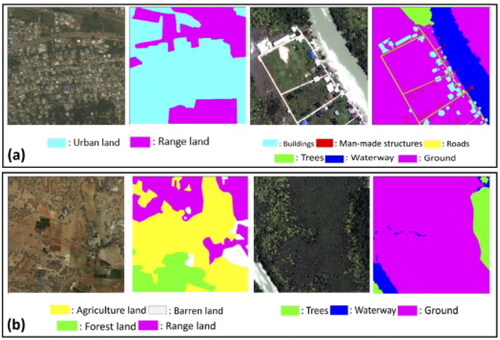
• Inconsistent training samples: Researchers in the RS community who want to do semantic segmentation are now able to use more crowd-sourcing or public datasets Demir et al. (2018) Schmitt et al. (2021). But the class definitions and amount of detail in these crowd-sourcing datasets or public benchmark datasets may not be the same. Figure 1 shows an example of a more detailed classification that separates buildings from other man-made structures. Some datasets define the ground class as including low-vegetation, grass, and barren land, while others separate the ground into range-land with low vegetation and barrens. So, the first problem with using this kind of data is figuring out how to change or improve their labels to fit specific needs and details about the classification jobs. Inconsistency is also caused by using different types of remote sensing data Sui et al. (2020) and also by having a data set with images consisting of different numbers of bands. Due to discrepancies in VHR data Jin et al. (2022) propose a multi-source data fusion technique that requires re-sampling to unify the spatial resolution. The technique filters training samples and has the ability to offer product correction at a fine resolution. The superpixel algorithm was adopted to correct unreliable information of multiple products into a new land cover fusion product. The technique performed well as it achieved an accuracy of 85.80% on Landsat images.

• Lack of quality training data: The majority of present machine learning models in RS tend to underestimate their accuracy because they are contaminated by poor and low-quality training data, as shown in Schmitt et al. (2021). The low-quality data anticipated for learning algorithms can be another obstacle, despite active efforts to address the issue, for example by feeding the community with new data as samples. Employing techniques such as image enhancement and restoration helps to deal with issues to do with lack of quality data. Image enhancement techniques such as Histogram equalizer, Linear congruent adjustment, etc. improve image quality balancing parameters with regard to contrast, brightness, and sharpness Kundu (2022). Image restoration techniques artifacts like noise or blurs from images.

Figure 1. Inconsistencies of the class definition and level of details, (Qin and Liu 2022).

2.3. Intra-class variability and inter-class similarity for VHR data

VHR data with a ground resolution of a meter or less have improved earth observation by providing more detailed information. The increased resolution has increased intra-class variability and inter-class similarities: spectral information alone can identify a pixel as belonging to multiple land cover classes, and different classes may contain pixels with similar spectral signatures Qin (2015). There was extensive research into possible solutions for this problem, such as object-based approaches or spatial-spectral characteristics Ghamisi et al. (2015), but the advances that were possible couldn’t keep up with the higher resolution and volume of data. Therefore, it may become more of a challenge when more sophisticated (and complex) models are utilized with larger numbers of annotated datasets. To tackle the problem of inter-class similarity and intra-class variance Venkataramanan et al. (2021) developed a model that automatically picks classes that are to be clustered and also determines an optimal number of classes to be generated. The obtained clusters are considered to be independent classes. Inter-class is dealt with by employing a triplet loss function to separate features between each class. Zhang et al. (2022) proposed a technique that tackles intra-class variance problems by developing a machine-learning model that organizes input instances as a graph. From the obtained graph, a normalized cut surrogate metric is used to determine intra-class variance within the training batch. The feature aggregation scheme is proposed by considering the equivalence between the normalized cut and random walk. The scheme is developed under the guidance of transition probability. Through supervision of aggregated features, transition probabilities are constrained to create a graph partition consistent with the given labels, hence the normalized cut and intra-class variance is well suppressed.

3. Proposed methods to handle VHR remote sensing images

The main obstacles to the current VHR RS picture classification are those already discussed. In addition to improving model performances, efforts have been made to solve these issues using multi-source/multi-resolution data, unlabeled data, more noise-tolerant models, and learning techniques. These initiatives can be generally described as follows:

• Weakly/Semi-supervised learning for small, imprecise, and incomplete samples.

  For weak supervision to work, the underlying training data must be inexpensive to collect (like publicly available GIS data) and noisy, imprecise, and asymmetrical. Because these methods attempt to incorporate heuristics, limitations, and error distributions, that are unique to each situation, hence they are not universal. This is because semi-supervised learning in RS assumes the existence of a large amount of unlabeled data and relies on the limited training data to achieve high classification performance, and is thus relevant to applications that deal with crowd-sourcing labels or labels with minor temporal differences Larochelle (2020). Li et al. (2017) proposed the zero-short scene classification (ZSSC) that has got the ability to recognize images even when presented with incomplete labeled data. The model is attributed to its capacity to recognize images from unseen scene classes. The approach utilizes, word2vec, a natural language process to map names of seen/unseen scene classes to semantic vectors. The relationship that exists between seen and unseen classes are defined with the help of a semantic-directed graph constructed from the semantic vectors. To perform knowledge transfer from seen classes to unseen classes, an initial label prediction on a test image is performed, then the label propagation algorithm is developed for ZSSC. The label-refined approach is adopted to suppress noise in the zero-shot classification results. The approach outperformed the state-of-the-art learning models in scene classification.

• Transfer Learning and domain adaptation to fill domain gaps.

  Within the realm of machine learning, transfer learning (TL) is defined as the presumption that knowledge gained from completing one task may be valuable if transferred to completing another task. A model that learns to conduct per-pixel semantic segmentation of scenes, for instance, has the potential to make human detection more accurate. In the field of RS, this term mostly refers to methods that aim to produce a generalizable classifier by minimizing gaps in the feature space. These methods can be applied to data collected from a variety of sensors in a variety of geographical locations. Pan et al. (2016) designed a multi-layer transfer learning that caters to specific latent features for domain adaptation. Firstly, the model generates specific latent features, which are then combined together into one latent feature space layer. Since the layers have different pluralism, multiple layers are generated to correspond to each distribution layer. The difference in the pluralism in each layer means that learning distributions from one layer helps learn distributions on other layers. The iterative algorithm based on Non-Nagative Matrix Tri-Factorization was adopted to solve the optimization problem. The multi-layer transfer learning managed to outperform state-of-the-methods on sentiment classification tasks.

• Use low-resolution photos or public GIS data as sources of tagged or partially labeled data.

  Nearly 80% of the world’s GIS data coverage is provided by OpenStreetMap, however, its quality varies Barrington-Leigh and Millard-Ball (2017), and some local governments make their GIS data available for public use. Researchers presented their work in this context and drew conclusions that were directly linked to the datasets. Additionally, these low-resolution labels can be used as a general guide to address domain gaps of data across various locations for scaling up the land cover classification of VHR data as the low-resolution labeled data with global coverage are gradually becoming more complete (e.g. National Land Cover Database Homer et al. (2012)). Wu et al. (2019) developed an effective unsupervised deep feature algorithm for classifying low-resolution images. The approach does not require any fine-tuning on the convenet filters and the convenet filters are used to extract features from both high and low-resolution images, and the obtained features are fed into a two-layer feature transfer network for knowledge transfer. The network has the ability to transfer distinguished features from a high-resolution feature space to a low-resolution feature space. The model was implemented on the VOC2007 dataset and showed significant improvement against baseline methods.

• Fusion of multi-modality and multi-view data. Unlabeled data sources such as Light Detection and Ranging (LiDAR), Synthetic Aperture Radar(SAR), and nighttime data can be used to study heuristics and improve latent representation learning Qin and Liu (2022). Lei et al. (2021) proposed a fusion of multi-modality and multi-scale attention network land cover classification of VHR images. The multi-modality fusion was designed on the basis of an encoding-decoding network that eliminates redundant features and fuses only useful features. This process increases the classification of land cover products by removing redundant features. The novel multi-scale spatial context enhancement module was adopted to improve feature fusion and alleviate the problem of large-scale variation of objects. The model was implemented on Vaihingen and Potsman datasets and performed well as it obtained F1-scores of 88.6 and 92.3% for Vaihingen and Potsman datasets, respectively.

3.1. Semisupervised learning (SSL) methods

One of the major challenges in Remote Sensing (RS) classifications is that the process of collecting VHR images for training (labeled) samples is really a tedious task. Therefore the RS science community has adopted SSL methods to tackle this challenge Yin et al. (2014); Bazi et al. (2012). SSL works by trying to generate a wealth of information from the available unlabeled data, despite having few available unlabeled data, with the aim of improving the performance of the classifier. Such approaches assume that points within the same structure are likely to have the same label Wang et al. (2015). In VHR images it seems reasonable to assume that if samples have close spectral information then they are likely to have similar labels. SSL methods have been successfully used in image classification applications such as vegetation mapping, land cover mapping, and urban planning Kwak and Kim (2023). Fan et al. (2020) proposed a semi-supervised multi-Convolutional Neural Network (CNN) ensemble learning method (Semi-MCNN) for urban land cover classification. The model harmonized the multi-CNN ensemble approach and a semi-supervised strategy to build an end-to-end architecture. This hybrid approach generally improves classification accuracy and generalization ability. The purpose semi-supervised technique was to leverage unlabeled images to labeled samples, and the ensembled teacher model dataset generation (EMDG), which is an automatic sample selection technique, was adopted to select appropriate samples and to generate large datasets from unlabeled samples automatically. The model was implemented on Shenzhen’s land cover data and performed well as it achieved an overall accuracy of 92.5%. Ekanayake et al. (2018) developed a semi-supervised approach for mapping boundaries between two vegetation zones using satellite hyperspectral data. The approach employed the Maximum Likelihood Classification technique in order to detect pure vegetation pixels. In order to determine the boundary between two major vegetation zones, the technique considers the degree of correlation of pixels containing vegetation at various spatial coordinates. Finally, the systematic procedure comprising Fisher’s Discriminant Analysis (FDA) and spectral clustering is used to divide the vegetation pixels into two vegetation zones.

3.2. Deep learning approaches

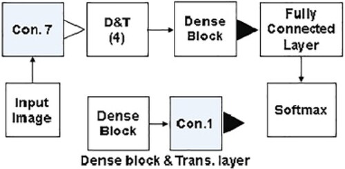
Deep learning technologies have been widely used to perform multi-class segmentation on VHR images Sertel et al. (2022). The number of classes to segment should be carefully examined prior to the application of deep learning technologies. Yuan et al. (2021) conducted a critical review on semantic segmentation using deep learning methods. The findings from the study showed that segmentation of VHR on datasets such as ISPRS vaihingen (five classes), ISPRS Potsman (five classes), and Massachusets (two classes) achieved high accuracy ranging from 85 to 99%. Audebert et al. (2018) developed an efficient multi-scale deep fully CNN based on ResNet and SegNet with multi-modal to perform segmentation on high-resolution remote sensing data. Results obtained showed that the fusion of multi-modal data significantly increases the accuracy of semantic segmentation by attributing its capability to learn multi-modal features jointly. Fu et al. (2017) integrated Atrous convolution to Fully Convolution Network (FCN) to build multi-scale network architecture to perform semantic segmentation on VHR images obtained from GF-2 and IKONOS datasets. The Conditional Random Fields were also added to the network in order to refine the output class maps. The model performed well as it obtained the precision, recall, and kappa values of 0.81, 0.78, and 0.83, respectively. Other developments such as Densely Connected Convolutional Network (DenseNet) Huang et al. (2017), and ShuffleNet Zhang et al. (2018) have been extended in remote sensing segmentation to address issues to do computational complexity, and these designs are producing satisfactory performance in semantic segmentation for remote sensing data Chen, Fu et al. (2018). DenseNet is an extension of ResNet, which introduced extra connections from one layer to its subsequent layers, and this has increased information flow and feature reusing Huang et al. (2017). The building blocks of DenseNet are dense block, which is made up of stacked layers of two filters (a 3 × 3 followed by a 1 × 1 filter. The dense blocks are interconnected with a 1 × 1 convolutional layer for feature dimensionality reduction. The network structure alleviates the vanishing gradient problem and enables feature reuse. Figure 2 shows the DenseNet architecture.

Figure 2. DenseNet architecture (Yuan et al. 2021).

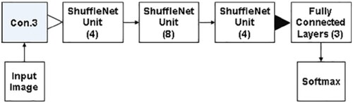
ShuffleNet Zhang et al. (2018) significantly increases computational complexity by reducing computation complexity of 1 × 1 convolutions and utilizes channel shuffle to help the information flow across feature channels. The computation of individual shares to be processed by the GPU is divided by the group convolution, and the output is reorganized into a matrix, where the rows are the group count and the columns are the channel count. The depthwise convolution is used instead of 3 × 3 convolution. The second group convolution restores channel dimensionality to match the residual for concatenation. Figure 3 shows the DenseNet architecture.

Figure 3. ShuffleNet architecture (Yuan et al. 2021).

3.3. Multi-resolution data classification

Multi-resolution data classification technique considers different levels of information granularity to analyze task data. This technique is widely used to perform classification tasks on data such as VHR images, graphs, and time series. It works by extracting patterns or features from images at different resolutions and integrating them into the classification performance. Duarte et al. (2018) developed a multi-resolution feature fusion for classifying building images using CNN. This approach integrates feature maps produced from different resolution levels (terrestrial, aerial, satellite) in order to categorize damages on building from remote sensing images. The results of the study demonstrated that multi-resolution fusion techniques outperform the traditional methods in classifying building images with 89% compared to 84%. The concept of using multi-resolution produces better accuracy and localization capability than using single-resolution features. Teruggi et al. (2020) proposed a hierarchical learning machine approach for multi-resolution 3D point cloud classification. The study extended the learning machine approaches with a multi-level and multi-resolution approach. The integration of the hierarchical concept optimized 3D classification results and improved the learning process. The multi-level and multi-resolution procedure was tested and assessed on two large datasets (the Pomposa Abby and Milan Cathedral both in Italy). The model managed to identify necessary architectural classes at each geometric resolution. Fixed network structures at a single resolution are difficult to characterize surface targets that have bright colors and different shapes with fixed sizes. To address this challenge Cong et al. (2022) proposed a structure defined by sample characteristic (SDSC) multi-resolution classification network that learns samples using a multi-resolution strategy and the principle of maximum classification probability. In order to improve the credibility and classification accuracy, the results obtained from the multi-resolution strategy were integrated into the final classification results. The proposed method is suitable for classifying high spatial resolution remote sensing images because of its better cognitive performance and insensitivity to noise.

4. GEOBIA studies

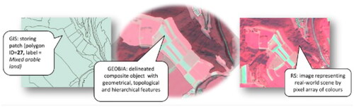
GEOBIA is a remote sensing tool used for land cover mapping and detecting land cover changes. It is a new discipline in remote sensing science that has evolved from pixel-based approaches and has significantly improved the workflow of imagery processing, particularly for land cover classification and detection Arvor et al. (2013). GEOBIA’s main goal is to deal with more complicated classes that are determined by spatial and hierarchical relationships both within and outside of the classification process Lang (2008). Of course, one might perform a multi-spectral classification in an RS system first, then group and rearrange the labeled pixels to construct objects using GIS software. However, the analyst may be skewed by this sequence, which limits the number of classes that may be handled. The outcomes achieved through this process differ from those that would be obtained with a single conceptual step, as is the case with human perception. Instead of examining the spectral behavior of individual pixels, the object-based approach groups adjacent pixels into objects, which then serve as the observation units. This classification circumvents the issue of artificially square objects as used in the per-pixel analysis Fisher (1997); Burnett and Blaschke (2003); Blaschke (2010), so long as the objects of interest cover a sufficient number of pixels to permit a meaningful representation of their shape. GEOBIA has been used in a range of applications such as geo-morphology Drăguţ et al. (2011), agriculture Vogels et al. (2017), archeology research Hegyi et al. (2020), and soil science Dornik et al. (2018). GEOBIA has managed to bridge the gap between remote sensing and Geographic Information Science (GIScience). In the fraternity of GIScience, the term Object Image Analysis (OBIA) was first introduced in 2006 Lang and Blaschke (2006), and later reformulated as GEOBIA in 2008 whose central focus was on Earth Observation (EO) applications and the integration of geo-spatial-temporal reasoning to deal with high volumes of EO imagery and other related information extraction challenges Lang et al. (2019). GIScience scholars have reached a consensus on the fact that GEOBIA is a paradigm shift Blaschke et al. (2014), that has managed to bridge the semantic information gap from big data in the image domain. The representation of 2D imagery as a gridded array of pixels does not provide descriptive content with regard to semantic information or object boundaries Lang et al. (2019). Such information needs to be documented in metadata. The image content in the current setup cannot be queried, but attempts to meet this vision exist Blaschke (2010). Geographic Information system (GIS) datasets are discrete and the finite vector set handles discrete categorical nominal variables rather than numerical variables Lang et al. (2019). The success of GEOBIA as measured by bibliometric measures Blaschke et al. (2014) is attributed to its mediating power between geospatial entities and continuous field representations, which caters to the needs of GIS and remote sensing communities. The Harmonisation of these two models is presented in Figure 4.

Figure 4. Impact of land cover type on the evolution of NPSS in the near-infrared (Lang et al. 2019).

The classification system of traditional pixel-based methods suffers from the salt and pepper-effect. This problem was alleviated by the Object-Based Image Analysis (OBIA) methodology when implemented on the Northern California vegetation inventory (Yu et al. 2006). OBIA adds object shape and context to spectral and textural information, and this significantly lowers the salt and pepper effect problem.

Another study by Chubey et al. (2006) used object-based analysis of IKONOS-2 imagery for extraction of forest inventory parameters rather than the traditional pixel-based image analysis approaches. Object-based analyses were first introduced in the area of remote sensing by Kettig and Landgrebe (1976), however, the approach did not receive much attention as its pixel-based method counterpart (Lu et al. 2013). Later, the object-based analysis techniques proved to be of significant importance in forest information extraction (Hay et al. 1996; Pekkarinen 2002; Imaging 2002). This was reinforced by the introduction of commercial object-based image analysis software such as eCognition (Arvor et al. 2019), feature analyst, etc. Chubey et al. (2006) developed a novel method that used the eCognition software and decision tree statistical analysis to extract forest inventory parameters. The IKONOS-2 images were segmented into image objects using the eCognition software. The multi-resolution segmentation was employed, where the image was partitioned into homogeneous multi-pixel regions. The size, spectral homogeneity, spatial homogeneity, and shape of the generated image objects were used to guide the segmentation procedure. The segmentation process was further tested against several other input/weighting combinations whereby each combination was evaluated on its ability to delineate meaningful landscape components. Image objects delineated carried crucial forest-related information that was derived from spectral and spatial characteristics of forest stand composition. Furthermore, analysis was performed using decision trees to determine correlations between image object metrics obtained from input data and individual forest inventory parameters. Decision trees were chosen because (a) they can handle high dimensional datasets, (b) they are able to work on both non-continuous and continuous variables, (c) of the non-parametric nature of the approach, and (d) they are easy to implement. However, there are some challenges with decision trees. Their performance depends on the quality and representation of training data (Friedl et al. 1999) and the accuracy increases with more training data. Therefore, the requirement for large training datasets is a concern from an operational perspective.

A quite number of studies have shown that OBIA methods are, re-applicable and more transferable to other images. This is achieved by re-applying the rule set on other conditions, and rule sets have the ability to adapt to new changed conditions. Hofmann et al. (2011) developed a new method to measure the robustness of a rule set. The new method is based on the assumption that the level of adaptation to be measured is in congruence with the quality of classification achieved. The robustness x_i of an unchanged rule set applied on an image M_i (i.e. = $Y=Y_I=Y_I$ is expressed by ratio of quality values: $x_i=\frac{q_i}{q_r}.$ If $x_i>1.0$ it implies a better result for M_i and vice versa for $x_i<1.0.$ The mean robustness of all the images M_n is expressed $x=\frac{1}{n}{\sum }_{i=r}^n(x_i)$ and the greater x the more Y for q_r > 0.

The studies in part delves into the importance of evaluating segmentation results and considered segmentation evaluation metrics such as the inverse of the number of objects (INO), Normalised Post Segmentation Standard Deviation, and Bhattacharyya Distance (BD) have been provided. A method for evaluating the quality of segmentation results in object-based classification was presented by Radoux and Defourny (2008). The proposed method constituted of two indices; one index was used to evaluate the extent to which the classification could be improved while the other assessed the boundary quality of the delineated land cover classes. Using a combination of three parameters from the same segmentation technique, the method was used to segment a Quick-bird image. It was established that large groups of pixels in an image, aid in the reduction of variance (Edwards and Cavalli-Sforza 1965). The study opted for a small intra-class variance with the assumption that it improves parametric classification. Over and under-segmentation were assessed using indices based on mean-sized objects. As a first quantitative goodness metric, the inverse of the Number of Objects (INO) was utilized. INO measures the ability of a model in segmenting an image into individual objects. INO is expressed as $\mathit{INO}=1/N$ where N represents the number of objects. The second global index was the Normalised Post Segmentation Standard Deviation (NPSS). It examines segmentation quality based on the variability of the segmented image against the variability of the entire image. NPSS is expressed as $\mathit{NPSS}=(\sigma s-\sigma x)/\sigma x$ where σs is the standard deviation of the pixel intensity values in the segmented region and σx is the standard deviation of the intensity values of the whole image (that is it includes both the segmented region and non-segmented region. The NPSS was used to calculate the class uniformity by replacing each pixel value with the parent object’s mean values. The small intra-class variance does not always improve classification results; in some circumstances, a considerably large variance between two classes can improve the classification. Therefore, a dissimilarity metric, the Bhattacharyya Distance (BD) was co-opted in the study to test the relevance of the proposed goodness indices since it contains the term that compares co-variance matrices and it also accounts for classification errors (Webb 2003). BD is a measure of dissimilarity between two probability distributions. For probability distribution p and q on the same domainX, BD is expressed as $DB=-ln(BC(p,q))$ where $(BC(p,q))=\sum _{x\in X}\sqrt{p(x)q(x)}$ where p(x) and q(x) are probability density functions.

Artifacts along the boundaries and missing boundaries are the key challenges with segmentation algorithms. The quality of segmentation precision is determined by the number of artifacts along the boundary. The accuracy and precision criteria proposed by Mowrer and Congalton (2000) were utilized to evaluate the positional quality of the edges. The bias and mean of the distribution of boundary errors were used to determine the accuracy and precision, respectively. Figure 5 shows sample errors along the edges of a segmentation result. Negative values were assigned to non-matching polygons (omission error) and positive values to matching cases. The goodness of indices was evaluated by NPSS and BD. Both indices gave valuable insight into segmentation findings. Results showed that NPSS was more correlated than INO. The positive results can be attributed to the fact that the mean class values were not modified by the segmentation. However, segmentation parameters were shown to be sensitive to global NPSS, with the object size parameter accounting for more than 80% of the variance. The effect of segmentation on every NPSS class had to vary, this reflects the sensitivity of segmentation algorithms to the land cover class. The absolute boundary error was sensitive to under-segmentation and was able to detect artifacts along class boundaries. There was a higher correlation $(R^2>0.94)$ between shape parameters and boundary errors. Results from Table 1 show the average absolute errors of parameters in various scales smooth, mixed, and compact. The studies have revealed that most segmentation algorithms face challenges that include artifacts and missing values along the boundaries that deter them from achieving good segmentation results. Evaluation metrics such as NPSS, INO, BD, accuracy, and precision for assessing segmentation quality were looked at in these studies.

Figure 5. Errors along the edges of a segmentation output. Black polygons are omissions (−) and white polygons are commissions (+) with respect to class 1 (Xie et al. 2008).

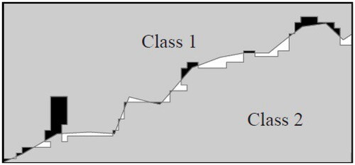
Table 1. Average of absolute errors (in meters) on boundary position between deciduous and coniferous forests, for a combination of segmentation parameters, i.e. scale parameter between 10 and 60 and compactness, illustrated for forest/arable land interfaces (Xie et al. 2008).

Scale	10	20	30	40	50	50	Mean
Smooth	2.3	3.4	4.1	4.7	5.3	5.7	4.3
Mixed	2.2	3.2	3.8	4.3	4.8	5.3	3.9
Compact	2.1	3.0	3.7	4.2	4.7	5.1	3.8

A study by Osio et al. (2018) uses OBIA-based monitoring of Riparian vegetation to assess the effect of flooding on the Lake Nakara Riparian Reserve vegetation species. An OBIA methodology was proposed (Osio et al. 2018) to serve as the basis for the classification of Riparian vegetation. The methodology comprised four pillars: data capture, pre-processing, processing, and analysis. Satellite data was downloaded from the USGS site, from Landsat 5 TM, Landsat 8 OLI (collected in 2014), and Landsat 8 OLI (collected in 2016) datasets. The pre-processing consisted of removing noise and ensuring uniformity between the datasets. The Ehlers fusion technique was employed to pen sharpen each image to 15 m resolution. Raw values of the images were converted to Top of the Atmosphere reflectance by the ArcGIS 10.4 software using a spatial analyst tool, in the arc toolbox. The planetary reflectance PY is defined as $PY=M_p{Q}_{\mathit{cal}}+A_p,$ where Q_cal is the quantized and calibrated standard product pixel value and M_p and A_p are the band-specific multiplicative and additive re-scaling factors, respectively. A multi-resolution segmentation algorithm was adopted to convert pixels into image objects. Four bands namely; green, red, near-infrared (NIR), and shortwave infrared (SWIR) were used to classify vegetation indices on each dataset. NDVI values were obtained from the rule set established in the feature view and the supervised classification was carried out for each image using the K-NN algorithm. In terms of classification scales, scaling varied across different images such that there were different numbers of instances per imagery. Multi-resolution segmentation was used to segment images into image objects based on the feature parameters of layer weights, scale parameters, and composition of homogeneity criterion. The parameters were set in eCognition Developer 9.2 and were used by the multi-resolution segmentation to divide the image into homogeneous objects. Table 2 shows the segmentation scales set.

Table 2. Segmentation scales (Osio et al. 2018).

Image	Scale	Shape	Compactness	Red	Blue	Green	NIR
Landsat5TM–2011	5	0.2	0.7	1	1	1	1
LandsatOLI–2014	40	0.5	0.5	1	1	1	1
LandsatOLI–2016	20	0.2	0.7	1	1	1	1

Hossain and Chen (2019) reviewed object-based image segmentation algorithms and challenges from remote sensing perspectives. The authors concluded that the quality of image segmentation has a significant impact on the final feature extraction and classification in OBIA (Hossain and Chen 2019; Vickers 2017; Su 2017). Many other studies (Blaschke et al. 2008; Cheng et al. 2001; Zhang et al. 2017) argued that the most crucial step in OBIA is image segmentation. Geographic Object Image Analysis (GEOBIA) was established to provide for image analysis by remote sensing scientists, environmental disciplines, and GIS specialists (De Jong and Van der Meer 2007). A comprehensive review of studies related to GEOBIA was undertaken by Blaschke (2010).

Chiu and Lin (2005) formulated the mathematical definition of segmentation as follows: given P, the homogeneity criteria and R, an entire image; R_i and R_j are segments of R if the following conditions hold (1) $R_i\subseteq R,$ (2) $R=U_i=1,\dots ,n,$ (3) $R_i\cap R_j=\theta$ and (4) $P(R_i\cup R_j)=\mathit{false},$ where i = j and R_i and R_j are neighbours. Segmentation algorithms have been categorized into (a) pixel-based (Friedl et al. 1999), (b) edge-based, (c) region-based, and (d) hybrid-based (Beveridge et al. 1989). In edge-based segmentation, the algorithm determines the edges, which are boundaries between objects (Cao et al. 2016); the edges are then closed up by continuous algorithms (Martin et al. 2004). Filtering, enhancement, and detection are the three key processes in edge detection (Jain et al. 1995). Filtering methods are necessary as they produce minimum blurring edges (Jain et al. 1995; Chen et al. 2006; Sahin and Ulusoy 2013). Enhancement highlights the pixels with huge changes in local intensity levels, and the enhanced data is utilized to detect real or genuine edges. The next stage is to use techniques like Hough transform (Kiryati et al. 1991), neighborhood search (Ghita and Whelan 2002), and watershed transformation (WT) (Vincent and Soille 1991). For natural segmentation, WT is commonly utilized (Hossain and Chen 2019). The region-based segmentation starts from the inside of the image and goes outwards until reaching the object boundaries (Zhang et al. 2016). Merging and splitting are the two basic operations in region-based segmentation (Fan et al. 2005). The segmentation process follows a systematic approach (Bins et al. 1996): (a) the first step performs an initial (seed) segmentation of the image, (b) the next step merges adjacent segments that are similar while splitting those that are dissimilar and (c) the previous step is repeated until there are no more segments to merge or split. The region growing or merging is defined by two main issues (Lucchese and Mitra 2001): (a) selection of a seed region and (b) similarity. Algorithms such as K-means clustering (Wang et al. 2010), hybrid region merging, single-seeded region growing (Verma et al. 2011), Particle Swarm Optimization (PSO) method, etc. (Mirghasemi et al. 2013) are used to generate the initial seeds. However, researchers are still in search of algorithms that work without seeds (Wu et al. 2015) or that are influenced by neighbors, even though seeded (Fan et al. 2005). After seed selection, the region grows sequentially by adding similar pixels, guided by specific homogeneity criteria. The criteria determine whether the pixels belong to the growing region or not (Nock and Nielsen 2004). The region splitting and merging entails, using the homogeneity criterion (based on attributes such as grey values, texture internal edges, etc.) to split the image into several segments (De Jong and Van der Meer 2007). If the seed image is not homogeneous, then the image is split into four sub-regions which serve as seeds for the next level (Martin et al. 2004). The process continues until all sub-regions become homogeneous. Bottom-up and top-down strategies are combined in the split and merge method (Guindon 1997). Bottom-up approaches enlarge the image by combining or merging comparable pixels, whereas top-down approaches split an entire image into image objects depending on the heterogeneity criterion (Benz et al. 2004). Edge-detecting methods face problems in generating closed segments and are excellent in detecting edges, while region-based methods are good in generating closed segments but are imprecise in detecting edges (Wang and Li 2014). Hence an algorithm was proposed that harmonized segmentation using both edge and region-based segmentation maps inputs Chu and Aggarwal (1993). The technique utilized the maximum likelihood estimator to predict initial edge positions from multiple inputs. An iterative procedure is then employed to smooth the resultant edge patterns. Finally, the edge map is converted to a region map using closed-edge contours. The regions are then merged to ensure that every region has the required properties.

5. Challenges of GEOBIA

In the past two decades, GEOBIA has been successfully adopted for land cover mapping (Blaschke and Strobl 2001; Blaschke et al. 2014). However, GEOBIA techniques require that regions of interest or objects be identified before applying classification rules on extracted objects (Blaschke and Strobl 2001). The segmentation step either relies on user expertise or empirical training to be adapted for each new scene to be processed (Drăguţ et al. 2014; Ming et al. 2015). Hence, GEOBIA is not applicable for Big Geodata where there is a large scale analysis which requires methods that are super-fast and robust (Merciol et al. 2018). Furthermore, GEOBIA has not yet been quantitatively verified though there is a general consensus among numerous researchers (Tehrany et al. 2014).

GEOBIA has been extensively used in land cover mapping applications. Land cover mapping is a complicated process as it incorporates factors such as image type, segmentation methods, accuracy assessment, classification algorithms, input features, etc. that have a great influence in the quality of the final product (Khatami et al. 2016). It is still a huge problem to come with a standard GEOBIA technique that provides an optimal solution for every study area. Spatial resolution is inversely proportional to segmentation scales. Figure 6 shows the relationship between spatial resolution and segmentation scale.

Figure 6. Correlation between spatial resolution and segmentation scale (Cai et al. 2014).

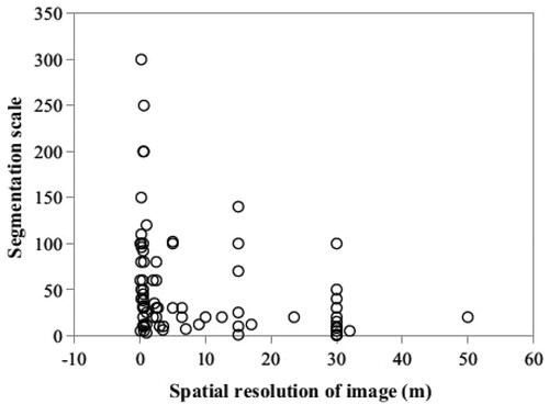
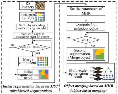
Whenever the spatial resolution becomes high, the segmentation scales become smaller and the lower the spatial resolution, the greater the configured optimal segmentation scales. It is very complex (Johnson and Xie 2011) to determine optimal segmentation scales due to the fact that the variability of the scale is affected by other image characteristics such as the size of the study area. The scale issue has emerged to be a huge problem for OBIA studies in relation to multi-segmentation scale methods. Therefore, there is a need to determine the appropriate segmentation scale necessary to obtain optimized segmentation results (Arbiol et al. 2007). Many researchers have explored trial and error approaches by varying segmentation scales based on their experience (Laliberte and Rango 2009), however, this approach is not advisable (Johnson and Xie 2011). In order to counteract this challenge Gu et al. (2018) propose an efficient multi-scale segmentation method based on graph theory and Fractal Net Evolution Approach (FNEA). The proposed model is shown in Figure 7. The contributions from this approach are that: (a) the Minimum Spanning Tree (MST) algorithm that performs the initial segmentation and the Minimum Heterogeneity Rule (MHR) algorithm adopted for object merging in FNEA are hybridized, (b) the segmentation strategy is implemented using data partition and the reverse searching forward processing chain using the Message Passing Interface (MPI) parallel technology. This approach is highly effective since it uses a fast graph segmentation algorithm and it also serves as a multi-scale segmentation and is hence suitable for a variety of landscapes such as industrial or agriculture. The problem of multi-scale segmentation also arises in defining semantic rules to relate lower landscape units to high-level organizations. To address this issue Burnett and Blaschke (2003) developed Hierarchical Patch Dynamics (HPD) framework that aids in the development of describing patterns and processes, acting through a range of scales, which make up landscapes. The framework was implemented on two different projects. In the first project, habitat mapping was done using a multi-scale GIS database. The landscape segments were generated using sub-patch information including dominant tree crown densities and species. In the second project, fractal-based segmentation was adopted to produce agricultural scene segments, and the decision framework was adopted to choose the best combination of segmentation levels to identify shrub encroachment.

Figure 7. Multi-segmentation based on MST and MHR Gu et al. (2018).

The next section presents recent developments in GEOBIA.

6. New GEOBIA developments

This section reviews new GEOBIA developments in terms of data sources, object based feature extraction, geo-object-based modelling frameworks, new forms of image objects, GEOBIA systems for novice GEOBIA users, and the use of knowledge from other disciplines.

6.1. Data sources

Modern high spatial resolution sensors provided a new landscape for remote sensing fraternity to study free-scale object or phenomenon from anywhere on the Earth’s surface Chen, Weng, et al. (2018). Ancient GEOBIA studies used to work with classic, single-image optical scenes for proof-of-concept studies, however new development in remote sensing fraternity have sharp increase of non-conventional data image type richer in spectral, spatial and temporal information, thereby, improving the modelling for geographical entities Chen, Weng, et al. (2018). Conventional GEOBIA data is defined as a high resolution imagery with limited spectral bands acquired by remote sensors mounted on relatively stable satellite/airborne platforms.

As depicted in Figure 8, rather than collecting images through satellite or airborne sensors, unmanned aerial system (UAS) or Drones have the ability to collect either sub-meter or sub-decimeter resolution data with high flexibility and very little demand for resources.

Figure 8. Conventional data types and image objects (Cai et al. 2014).

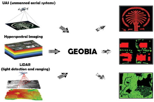
Similarly, Light Detection and Ranging (LiDAR) represents the conventional 2D spectral features with 3D structural information (bottom of Figure 8). Since segmentation in GEOBIA is solely applied to 2D imagery, LiDAR converts clouds or waveforms to raster format image models before they are used in GEOBIA framework. The GEOBIA community has taken the advantage of LiDAR’s penetration capacity of retrieving 3D structures of non-solid objects with gaps such as trees. Chen, Weng, et al. (2018) argued that the LiDAR approach resembles real forest structure than sharpened WorldView-2 optical imagery at a 0.5 m resolution.

Hyperspectral images have been extensively used by GEOBIA experts to distinguish between geographical objects of similar spectral characteristics. Traditionally, hyperspectral images comprised of very limited spectral range that spans from visible to near-infrared section of the electromagnetic spectrum. These types of images have been successfully used in classifying mangrove species with 30-band (Kamal and Phinn 2011), examining post-fire severity by utilizing a 50-band MASTER mosaic (Powers et al. 2015) and assessing tropical forest area diversity with a 129-band AisaEAGLE imaging spectrometer (Schäfer et al. 2016). Hyperspectral imagery (middle of Figure 8) is very rich in spectral information as compared to multispectral imagery data sets, hence the extra bands can be used to obtain other useful information such as textural, object-based shape and contextual features. However, obtaining this extra information aids in computational costs due to rigorous analysis for feature extraction. Advances in sensor technology is moving towards extending spectral information beyond the red, green, blue and near-infrared segment of the spectrum, e.g. Worldview-2 has additional coastal-blue (400–450nm), yellow (585–625nm), red-edge (705–745nm) and near-infrared-2(840–1040nm) bands at the 1.84 m resolution Vermeulen and van Niekerk (2016).

6.2. Object based feature extraction

Classic features such as texture, context measures and spectral have been extracted through unsupervised image segmentation. GEOBIA has progressed to solely obtain these features through analyzing characteristics of geographic objects.

6.2.1. Novel object features

The traditional way of characterizing features of individual regions of interest involves measuring shape complexity (Mowrer and Congalton 2000; Cao et al. 2016), extracting features from interval-valued data modeling (He et al. 2016a), and establishing semivariogram descriptors for quantifying spatial correlation and patterns within objects as presented in Figure 9. A study by Wang et al. (2017) extended the approach to include the relationship between objects and lines. The authors explained that geographical objects in urban setups have more regular shapes than natural environments and have systematically distributed lines. Cai et al. (2014) extracted geostatistical features by examining the temporal behavior of each object’s internal structure in relation to object based-based change detection.

Figure 9. Object-based features obtained from three scales (a) image-objects (b) neighborhood image objects and (c) individual communities (Cai et al. 2014).

A study by Wang et al. (2017) extended the approach to include the relationship between objects and lines. The authors explained that geographical objects in urban setups have more regular shapes than natural environments and have systematically distributed lines. Cai et al. (2014) extracted geostatistical features by examining the temporal behavior of each object’s internal structure in relation to object based-based change detection. Chubey et al. (2006) proposed to incorporate neighboring image objects to improve the description of contextual information. Chen et al. (2011) came up with a geographic object-based image texture (GEOTEX) model that produced a set of texture measures by examining each image object with its corresponding neighbors through the natural window/kernel.

In GEOBIA techniques, the segmentation process produces a large number of object-based features (Figure 9), thereby reducing computational efficiency and also increasing modeling uncertainties. To mitigate this challenge, Powers et al. (2015) harmonized Principal Component Analysis (PCA) and Minimal Noise Reduction (MNR) to reduce the airborne MASTER sensor’s 50 input spectral bands prior to segmentation.

6.2.2. Feature selection space

Techniques ranging from statistical analysis to machine learning and deep learning have been employed to obtain optimal features through the reduction of feature space. The majority of these techniques follow the approach of minimizing the number of input features while at the same time maximizing follow the separation distance between classes. Once processed features are then ranked in order of significance. Machine learning approaches have evolved for feature space reduction. However, for GEOBIA techniques, a consensus has not yet been reached as to which machine learning algorithm is the best for feature space reduction relative to particular applications. Algorithms that have been applied successfully for object-based feature selection include: Winnow (Littlestone 1988; Powers et al. 2015), random forest (Breiman 2001; Franklin et al. 2000), minimal redundancy maximum relevance (Peng et al. 2005) and Support Vector Machine (SVM) (Huang and Zhang 2013). Generally, the choice of algorithm for optimal feature space reduction depends on performance, ease of use, and accessibility. With the aim of improving feature selection from VHR images Chaib et al. (2022) proposed a framework based on Vision Transformer (ViT) models. Firstly, the ViT model is used to extract informative features from the VHR image scene, and the obtained features are merged into one signal dataset. The feature and selection algorithm is then adopted to trim off features that do not provide information to describe scenes such as beaches and agriculture. These features have a tendency of degrading the classification accuracy. The proposed model outperformed other state-of-the-art models when implemented on the VHR benchmark. Chen et al. (2016) proposed an efficient semi-supervised feature selection (ESFS) technique that selects all the desirable features by exploiting all the details available on the unlabeled objects. Firstly, it uses the probability matrix of unlabeled objects in the loss function to obtain features that are relevant per each class, instead of using traditional graphs. Lastly, norm regularization is employed to ensure that selection matrix rows have the required sparsity. ESFS outperformed other classical methods when implemented on a VHR image. Too and Abdullah (2021) proposed an improved genetic algorithm (GA) that incorporates the performance of GA in feature selection. The approach uses the competition strategy that integrates the new selection and cross-over schemes to improve the global search capability. Also, the dynamic mutation rate is also incorporated to improve the search power of the algorithm in the mutation process.

6.3. Geo-object based frameworks

GEOBIA has been dominantly used in land-cover/use classification. Recently it has also been successfully used to detect features in the area of archaeological remains (Lasaponara et al. 2016), green roofs (Theodoridou et al. 2017), alluvial fans (Pipaud and Lehmkuhl 2017), and dunes (Vaz et al. 2015). Various modifications have also been employed with the aim of meeting specific needs in real-world applications. Eckert et al. (2017) improved the classification of fine geographical objects which only existed in certain landscape zones. Another study by Guo et al. (2013) enrolled a two-step strategy to enhance classification by using object-neighbour context and scene context, respectively. However, these methods lack the ability to analyze latent spatial phenomenon. This challenge was addressed by Lang et al. (2008) who introduced geons which serve as a spatial units that are homogeneous in terms of varying space time phenomena under policy concern. Lang et al. (2014) further improved geons and came up with composite geons which provided solutions to policy-relevant phenomena such as societal vulnerability to hazards. The GEOBIA framework relied on geo-object based basic principles to derive image-object classes. However, improvement was done on GEOBIA workflow by adding parametric and non-parametric models to analyse object based variation within a specific class.

6.4. New forms of image objects

Considering the fact that the 3D geographical objects are represented as image objects in 2D format, some uncertainties and errors in identifying ground features could arise as some spatial dimensions are neglected (Alexander et al. 2010). Techniques in remote sensing and computer vision have progressed to the extent that it is now possible to capture geographical objects in 3D (Vaz et al. 2015). New trend in GEOBIA methods now incorporates vertical features in GEOBIA modelling e.g. carbon estimation at the tree cluster level using canopy height from a LiDAR sensor (Godwin et al. 2015). Extraction of object features by these techniques was centred on calculating boundaries of 2D image objects (Godwin et al. 2015; Zhang et al. 2013). Remote sensing science fraternity now advocates for generating image object features directly from a 3D scene model, which accurately represents real-world geographical objects. Photogrammetry and computer vision techniques can be used to construct 3D scene models (Luhmann et al. 2019). Using 3D information to delineate objects boundaries still remains a challenging task, as it is possible to loose crisp boundaries for certain components, for instance, a transition zone between wetland and water (Bian 2007). Defining fuzzy boundaries seemingly provides a better solution, whereby an image object is treated as homogeneous unit and equal parts (in terms of homogeneity) have a possibility of belonging to a certain class.

6.5. GEOBIA systems for novice GEOBIA users

GIScience and other communities took two decades to adopt GEOBIA frameworks and software packages (Chen, Weng, et al. 2018). The GEOBIA experts play a major role in incorporating user’s knowledge and experience when developing GEOBIA models in order to achieve high accuracies. For GEOBIA applications to have a wider coverage, GEOBIA models should provide a way of translating novice-GEOBIA users understating of geographical entities into an appropriate choice of algorithms. This could be achieved with systems that have three key components such as (1) data query, (2) processing chain and (3) product sharing which can interactively direct a user to go through the entire GEOBIA process. Krizhevsky et al. (2012) argued that the translation of novice-GEOBIA understanding to GEOBIA language can be facilitated by the use of rule sets that are clearly defined and trained by machine or deep learning methods.

6.6. Embracing knowledge from other disciplines

GEOBIA has been extensively used in several disciplines (e.g. forest, urban planning, etc.), a gap still exists on how to integrate these disciplines to effectively support geo-object-based modelling (Chen, Weng, et al. 2018). Because of the nature of image analysis, GEOBIA hugely benefits from knowledge forecasting provided by computer vision that simulates human perception of digital imagery (Blaschke et al. 2014). Insufficient information on spectral, spatial, or temporal resolutions may result in experienced photo interpreters or computer programs producing incorrect perceptions of geographic entities (Castilla and Hay 2008). A potential solution proposed by Castilla and Hay (2008) is to take advantage of the Earth-centric nature of GEOBIA, where perceived geo-objects and their corresponding spatiotemporal dynamics meet rules or laws in natural or built-in environments. In a study on vegetation transitional zones from dense to bare ground in California by Chen, Weng, et al. (2018), a GEOBIA framework was employed to map disease-caused mortality and the results obtained indicated that there was over-estimation on patches of dead trees due to similar textural, geometrical and spectral characteristics between dead tree crowns and ground/shrub grass.

In order to enhance effective knowledge exchange and management, the GEOBIA community has adopted ontologies for specific applications (Andrés et al. 2017; Baraldi et al. 2017). Ontologies have played an important role in GEOBIA frameworks, but there is still a lack of comprehensive and universally accepted GEOBIA framework that provides guidelines for formalizing expert knowledge with ontologies. The next section discusses the use of ontologies in GEOBIA.

7. Ontologies for forest remote sensing image classification

Although data-driven approaches have attracted significant interest in research, knowledge-driven approaches remain an important future direction for the remote sensing (RS) science community Arvor et al. (2019). With that in regard, ontology having a strong power in knowledge representation, inference of common sense, knowledge sharing, and semantic cognition has gained much attention in the RS community Li et al. (2022). The Thailand Flora Ontology (TFO) (Panawong et al. 2018) was proposed to establish a semantic lexicon on the web, to assist plant biologists in the discovery of flora knowledge. The development of the ontology was against the backdrop that ordinary non-botanist people were not able to understand or receive accurate information about plants because plant information was expressed in English with botanical terms. Two steps were followed to design the ontology including the domain analysis for knowledge organization and the ontology development process. In the first step, a qualitative research method was employed to construct the Flora of Thailand knowledge structure, through (1) selection of already existing resources pertaining to plant ontology, biological classification, the flora of Thailand, and plant taxonomy, (2) flora content analysis from selected resources, (3) adoption of domain analytic approach for the organization of Thailand’s Flora, and (4) explicit clarification of flora knowledge organization in consultation with domain experts. The ontology development process requires ontology engineers and developers to have the requisite knowledge in ontology specification and ontology development environment (Chansanam and Tuamsuk 2016). The construction of the TFO ontology followed the guidelines suggested in Ontology Development 101 by Noy and McGuinness (2001). The scope of the TFO ontology was limited to the Flora of Thailand, therefore the study recommended further development into an ontology-based retrieval system.

A study on ontology-based semantic mapping for integrating land cover products using hybrid ontology was presented by Zhu et al. (2021). The integration of land cover data depended on the characteristics of land cover products such as the thematic information, spatial resolution, temporal frequency and accuracy (Zhu et al. 2021). The integration was performed at the data and schema levels. The schema level integration used the Ontology-Based Data Integration (OBDI) approach. The OBDI has different variants: single-ontology schema-level, multiple-ontology, hybrid and Global-as-View ontology approaches (Ekaputra et al. 2017). The choice of the appropriate OBDI variant for land cover mapping and integration remains a key challenge. The study involved the use of multiple land cover products whose data sources had different semantics for land cover concepts. Therefore, the hybrid approach for ontology construction was adopted because of the heterogeneity of the data sources. Each land cover data source resulted in a distinct ontology. These local ontologies were subjected to a mapping process with the help of the EAGLE concept (Zhu et al. 2021). Figure 10 shows the OBDI structure. The global vocabulary construction was done by following the EAGLE matrix (Zhu et al. 2021). Firstly, the data source is refined to meet the specific requirements of the definitions of different land cover types. Thereafter, the characteristics that suit a given cover type are arbitrarily chosen for the construction of local ontologies. The land cover type integration is facilitated by adding the axioms and attributes to reduce design inconsistencies. The conceptual description of each data source is explicitly done by local ontologies. Terms of interest of each data source and the hierarchical relationships between classes are analyzed. Then, local ontologies of land cover concepts are disintegrated to express the attributes and relationship clearly.

Figure 10. Ontology construction diagram (Zhu et al. 2021).

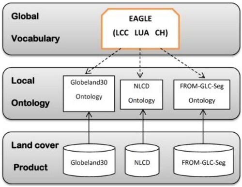
Figure 10 shows the three building blocks of the EAGLE matrix, that is, the land cover component (LCCs), land use attributes (LUA), and further characteristics (CH). Moving down the matrix, there is grain granularity, whereby the grain is refined going down in order to meet the requirements of the definition of the different scales of land cover types. The ontology of a particular land cover product can be designed by choosing an appropriate combination of components, attributes, and characteristics from the EAGLE matrix. The EAGLE matrix is extended to describe the main components and the relationship between them. Figure 11 shows the architecture of the EAGLE matrix. The conceptual model of the data source is described using a local ontology. All the required data sources are carefully examined by assessing the terms of each data source and the hierarchical relationship between each class. Finally, the ontology cover of each concept is broken into the global vocabulary-EAGLE matrix to clearly express the relationship between attributes. The land products considered in this example include NLCD, Glodeland30, and FROM-GLS-seg. The classes in the land cover product are organized in a hierarchical structure. Figure 12 shows an example of a coniferous forest in the local ontology of FROM-GLC-seg.

Figure 11. Structure of EAGLE matrix showing three blocks of land cover components (LCC), land use attributes (LUA), and characteristics (CH) (Smith and Hazeu 2015).

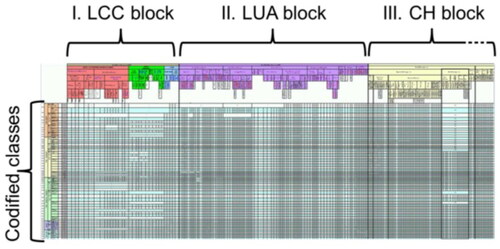
Figure 12. Coniferous forest in the local ontology of from-GLC-Seg. (Zhu et al. 2021).

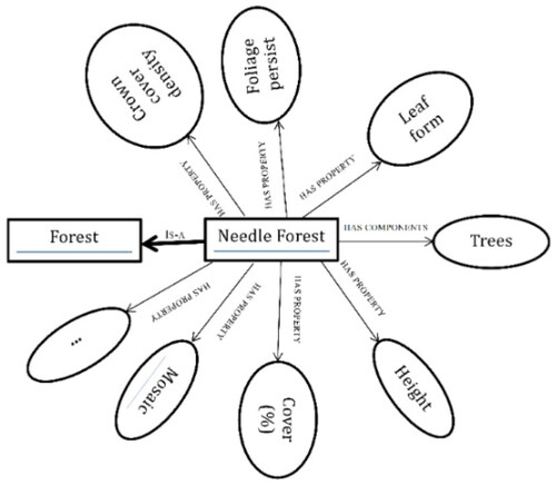
A study in Li et al. (2022) proposed a collaborative boosting framework(CBF) that integrates a deep learning approach and a knowledge-driven ontology reasoning module for remote sensing image semantic segmentation. The approach consists of two main modules, that is, the deep learning module based on the semantic segmentation network (DSSN) and the ontology reasoning module. The ontology reasoning module’s role is to establish a connection between intra- and extra-taxonomy reasoning in series. The intra-taxonomy reasoning module is incorporated to correct misclassifications done by the DSSN thereby improving the interpretability of the classification. On the other hand, the extra-taxonomy reasoning module works on the corrected results in order to provide refined details that will help DSSN make reliable interpretations. The two modules in the model interact iteratively until the output from the entire system is optimized. The CBF model’s primary focus is on predicting information relating to elevation and shadow on the basis that the predictions by the extra-taxonomy reasoning are sufficiently accurate for the DSSN.

8. State of the ontology-based model for forest image classification

A state-of-the-art model based on ontology and a deep learning model in Kwenda et al. (2023) was employed to classify forest images into their respective categories. The basis of this study was derived from the notion that integrating ontologies and semantic relationships significantly increases image classification accuracy. The model is composed of three main phases, that is (1) feature extraction, (2) ontology building, and (3) image classification. The model is presented in Figure 13.

Figure 13. The proposed model.

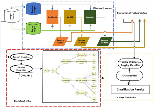
8.1. Feature extraction

In image processing tasks features play a critical role in image classification. The ensemble of ResNet50, VGG16, and Xception deep learning approaches was used to generate a set of features from the training data set. Features produced by each deep learning technique were aggregated together to produce the final feature vector. The ensemble approach generates features that produce more accurate results than those generated by a single approach.

8.2. Ontology building

The process of building ontology was synthesized through concept extraction and relation generation. Concepts relating to forests were established and the associated relationships between the concepts were generated. The semantic relationship between image classes helps train images for classes and this is accomplished by grouping together images belonging to a particular class. Image that belongs to a particular class C_i denoted as x_i implies that x_i is a child of C_i. Suppose that ‘artificial crop vegetation’ and ‘natural crop vegetation’ are the superclasses at the root node, the semantic rules will categorize images of ‘field’ and ‘orchard’ to ‘natural vegetation node’ even though both nodes belong to the ‘Primary Vegetative Area’ parent class (Figure 14). The relationship between two concepts is shown with a relationship arrow that joins the concepts together, e.g. an arrow from ‘orchard’ concept to ‘Artificial crop Vegetation Concept’ implies that ‘orchard’ is_– a ‘Artificial crop Vegetation’. The type of relationships considered in the study were hyponymy and hypernymy relationships. The generated ontology is shown in Figure 14.

Figure 14. Ontology of Forest types Kwenda et al. (2023).

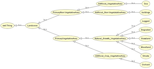
8.3. Image classification

The set of features generated by the ensemble of deep learning approaches was used to train a one-vs-all Support Vector Machine (SVM) classifier for each classifier so that each class could be distinguished from other classes. The classification of a given test image is performed by both hyponymy and hypernymy classifiers as illustrated in Figure 15. A given test image is assigned to a class with the best hypernymy classifier (artificial_– crop_– vegetation and the best hyponymy classifier (grassland). If the classifiers have a direct relationship, then their output will be merged together else the hyponymy classifier will be considered.

Figure 15. Classification using merging classifiers Kwenda et al. (2023).

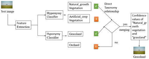
8.4. Evaluation metrics for the state-of-the-Art model

Metrics such as confusion matrix, Root Mean Square Error (RMSE), Accuracy, and Receiver Operating Characteristics Area Under the Curve (ROC_– AUC) were used to evaluate the model. Accuracy returns a ratio of correctly predicted classes to the number of samples evaluated. The definition of accuracy is presented in Equation (1)(1) $$\mathit{Accuracy}=\frac{TP+TN}{TP+TN+FP+FN}$$(1) . (1) $$\mathit{Accuracy}=\frac{TP+TN}{TP+TN+FP+FN}$$(1)

Where TP, TN, FP, and FN represent true positives, true negatives, false positives, and false negatives respectively. The area under the ROC curve is generally used to assess comparisons between learning algorithms, as well as the establishment of an optimal learning model. The AUC values rank the performance of the classifier. The AUC is presented in Equation (2)(2) $$\mathit{AUC}=\frac{s_p-n_p(n_n+1)/2}{n_p{n}_n}$$(2) . (2) $$\mathit{AUC}=\frac{s_p-n_p(n_n+1)/2}{n_p{n}_n}$$(2)

Where s_p is the sum of positive ranked samples, n_n, n_p denotes the number of negative and positive samples respectively. RMSE returns the square root mean square of all errors. The RMSE is expressed as Equation 3(3) $$\mathit{RMSE}=\sqrt{\frac{1}{n}*\sum _{i=1}^n{(O_i-P_i)}^2}.$$(3) . (3) $$\mathit{RMSE}=\sqrt{\frac{1}{n}*\sum _{i=1}^n{(O_i-P_i)}^2}.$$(3) where O_i are the actual values and P_i are the predicted values. With a confusion matrix, it becomes very easy to identify classes with more mislabelled data than others by providing the visualization performance of the classifiers.

8.5. Results of the state of the art ontology-based model

Results shown in Table 3 indicate that the state-of-the-art model based on ontology outperformed baseline classifiers without ontology in terms of ROC_– AUC, RMSE, and Accuracy. The ontology-based model performed well in separating classes in relation to other models as it attained the highest ROC_– AUC value of 0.99. The model also recorded the lowest RMSE of 0.532 suggesting that the predictions made by the model were very close to the actual values.

Table 3. Quantitative comparison of models.

Model	Test images	Correctly classified	misclassified	ROC– AUC	RMSE	Accuracy
kNN	152	124	28	0.97	1.530	0.816
OntologicalBagging	152	146	6	0.99	0.532	0.961
RF	152	131	21	0.99	1.094	0.862
DecisionTree	152	98	54	0.81	2.090	0.645
SVM	152	135	17	0.98	1.048	0.888
GaussianNB	152	97	55	0.79	1.678	0.638

9. Future directions and recommendations

A study in Arvor et al. (2019) recommended two research directions for using ontologies in remote sensing science namely, (a) the modeling of ontologies with spatial reasoning and cognitive semantics and (b) the investigation of bottom-up vs top-down approaches. The study also advised that spatiotemporal information can be included in ontologies by adopting the principles of naive geography and cognitive geography during the development process. In fact, these principles reflect two primary roles of ontologies that are, the alignment of data with expert knowledge and the representation of common sense categorization based on expert conceptualization. The challenges of spatiotemporal ontologies to implement cognitive semantics was emphasized by Kuhn et al. (2007). The authors provided guidelines for developing geospatial ontologies that are more cognitive, including (a) the use of sound meaningful and suitable primitives, (b) the recognition of space and time as the foundational aspects of ontology because they correlate with human conceptualization, (c) use process-oriented rather than static structures, (d) harmonize realistic semantics and cognitive semantics, (e) allow perspectivism and relativism, (f) allow conceptual mapping to enhance human-computer interaction, and (g) consider contextualization of elements to relate the situational and individual settings. Though GEOBIA came as a relief to the remote sensing science community by providing solutions to the problems posed by pixel-based methods, its use in forest image analysis suffers a setback of localizing knowledge within a particular domain which is rarely transferable because it solely depends on expert knowledge Thus, forest image analysis and classification require expert knowledge from different facets of remote sensing professionals, which is rarely formalized and difficult to automate, The study recommends the adoption of ontologies for forest image analysis and classification as they promote knowledge sharing and the reuse of formalized remote sensing expert knowledge. This recommendation is supported in study Arvor et al. (2019) that ontologies in remote sensing provide a breakthrough in dealing with the complex definition of geographic concepts, handling a geographic concept’s vagueness and ambiguity, and managing sensory and semantic gaps. We recommend a hybridization approach of ontologies and Explainable Artificial intelligence (XAI) for image classification in remote sensing science thereby boosting domain expert confidence in the results produced. Such a hybrid approach provides an explicit explanation of how it reaches its conclusion. Production of features is to be performed by XAI, and classifiers trained through ontology are to perform the classification task.

10. Conclusion

This paper conducted a critical survey of GEOBIA methods for forest image detection and classification. A review of modern ontology-based remote sensing applications for forest image classification gave an insight into the power of ontologies to explicitly represent knowledge, thereby, improving the classification process. The shortcomings of GEOBIA such as failure to deal with segmentation scales, highly subjective because of computer-aided photo interpretation, and not being able to handle Big Geodata information were addressed, and the call for ontologies in remote sensing applications as a solution for GEOBIA problems was highlighted. The primary core of representing domain expert expression has attracted the adoption of ontologies in remote sensing applications. The study recommended the revamp of GEOBIA, by adopting a hybridization approach of XAI and ontological frameworks. Considering that XIA is not a black box in nature and it provides an explicit explanation of how they reach their conclusion, the study recommended the approach to be used for feature generation. In this regard, the domain expert’s confidence in the obtained results is raised. Feature vector from XAI is passed on to classifiers trained through an ontological framework to perform the final step of segmentation.

Acknowledgements

The authors thank the University of KwaZulu Natal for providing financial assistance in accessing all resources and tools required to undertake this study.

Disclosure statement

No potential conflict of interest was reported by the author(s).

Data availability statement

Data sharing is not applicable to this article as no new data were created or analyzed in this study.

References

- Adelabu S, Mutanga O, Adam E. 2014. Evaluating the impact of red-edge band from rapideye image for classifying insect defoliation levels. ISPRS J Photogramm Remote Sens. 95:34–41. doi: 10.1016/j.isprsjprs.2014.05.013.
- Alexander C, Tansey K, Kaduk J, Holland D, Tate NJ. 2010. Backscatter coefficient as an attribute for the classification of full-waveform airborne laser scanning data in urban areas. ISPRS J Photogramm Remote Sens. 65(5):423–432. doi: 10.1016/j.isprsjprs.2010.05.002.
- Andrés S, Arvor D, Mougenot I, Libourel T, Durieux L. 2017. Ontology-based classification of remote sensing images using spectral rules. Computers Geosci. 102:158–166. doi: 10.1016/j.cageo.2017.02.018.
- Arbiol R, Zhang Y, I Comellas VP. 2007. Advanced classification techniques: a review. Revista Catalana de Geografia.
- Arvor D, Belgiu M, Falomir Z, Mougenot I, Durieux L. 2019. Ontologies to interpret remote sensing images: why do we need them? GIScience Remote Sens. 56(6):911–939. doi: 10.1080/15481603.2019.1587890.
- Arvor D, Durieux L, Andrés S, Laporte MA. 2013. Advances in geographic object-based image analysis with ontologies: a review of main contributions and limitations from a remote sensing perspective. ISPRS J Photogramm Remote Sens. 82:125–137. doi: 10.1016/j.isprsjprs.2013.05.003.
- Asma SB, Abdelhamid D. 2020. An object-based approach to VHR image classification. In 2020 Mediterranean and Middle-East Geoscience and Remote Sensing Symposium (M2GARSS), Tunis, in Tunisia; IEEE. p. 93–96. doi: 10.1109/M2GARSS47143.2020.9105140.
- Audebert N, Le Saux B, Lefèvre S. 2018. Beyond RGB: very high resolution urban remote sensing with multimodal deep networks. ISPRS J Photogramm Remote Sens. 140:20–32. doi: 10.1016/j.isprsjprs.2017.11.011.
- Baraldi A, Tiede D, Sudmanns M, Belgiu M, Lang S. 2017. Systematic ESA EO level 2 product generation as pre-condition to semantic content-based image retrieval and information/knowledge discovery in EO image databases. In Proceedings of the 2017 Conference on Big Data from Space; Luxembourg: Publications Office of the European Union Luxembourg. p. 17–20.
- Barrington-Leigh C, Millard-Ball A. 2017. The world’s user-generated road map is more than 80% complete. PLOS One. 12(8):e0180698. doi: 10.1371/journal.pone.0180698.
- Bazi Y, Alajlan N, Melgani F. 2012. Improved estimation of water chlorophyll concentration with semisupervised gaussian process regression. IEEE Trans Geosci Remote Sensing. 50(7):2733–2743. doi: 10.1109/TGRS.2011.2174246.
- Benz UC, Hofmann P, Willhauck G, Lingenfelder I, Heynen M. 2004. Multi-resolution, object-oriented fuzzy analysis of remote sensing data for GIS-ready information. ISPRS J Photogramm Remote Sens. 58(3–4):239–258. doi: 10.1016/j.isprsjprs.2003.10.002.
- Beveridge JR, Griffith J, Kohler RR, Hanson AR, Riseman EM. 1989. Segmenting images using localized histograms and region merging. Int J Comput Vision. 2(3):311–347. doi: 10.1007/BF00158168.
- Bian L. 2007. Object-oriented representation of environmental phenomena: is everything best represented as an object? Ann Assoc Am Geograph 97(2):267–281. doi: 10.1111/j.1467-8306.2007.00535.x.
- Bins LS, Fonseca LG, Erthal GJ, Ii FM. 1996. Satellite imagery segmentation: a region growing approach. Simpósio Brasileiro de Sensoriamento Remoto. 8(1996):677–680.
- Blaschke T. 2010. Object based image analysis for remote sensing. ISPRS J Photogramm Remote Sens. 65(1):2–16. doi: 10.1016/j.isprsjprs.2009.06.004.
- Blaschke T, Hay GJ, Kelly M, Lang S, Hofmann P, Addink E, Feitosa RQ, Van der Meer F, Van der Werff H, Van Coillie F, et al. 2014. Geographic object-based image analysis–towards a new paradigm. ISPRS J Photogramm Remote Sens. 87(100):180–191. doi: 10.1016/j.isprsjprs.2013.09.014.
- Blaschke T, Lang S, Hay G. 2008. Object-based image analysis: spatial concepts for knowledge-driven remote sensing applications. Dordrecht, Netherlands: Springer Science & Business Media.
- Blaschke T, Strobl J. 2001. What’s wrong with pixels? Some recent developments interfacing remote sensing and gis. Zeitschrift für Geoinformationssysteme. 14(6):12–17.
- Breiman L. 2001. Random forests. Mach Learn. 45(1):5–32. doi: 10.1023/A:1010933404324.
- Burnett C, Blaschke T. 2003. A multi-scale segmentation/object relationship modelling methodology for landscape analysis. Ecol Modell. 168(3):233–249. doi: 10.1016/S0304-3800(03)00139-X.
- Cai S, Liu D, Sulla-Menashe D, Friedl MA. 2014. Enhancing Modis land cover product with a spatial–temporal modeling algorithm. Remote Sens Environ. 147:243–255. doi: 10.1016/j.rse.2014.03.012.
- Cao W, Li J, Liu J, Zhang P. 2016. Two improved segmentation algorithms for whole cardiac ct sequence images. In 2016 9th International Congress on Image and Signal Processing, BioMedical Engineering and Informatics (CISP-BMEI), Datong, China; IEEE. p. 346–351. doi: 10.1109/CISP-BMEI.2016.7852734.
- Castilla G, Hay G. 2008. Image objects and geographic objects. In: Blaschke T, Lang S, Hay GJ, editors. Object-based image analysis. Lecture notes in geoinformation and cartography. Berlin, Heidelberg: Springer; p. 91–110.
- Chaib S, Mansouri DEK, Omara I, Hagag A, Dhelim S, Bensaber DA. 2022. On the co-selection of vision transformer features and images for very high-resolution image scene classification. Remote Sensing. 14(22):5817. doi: 10.3390/rs14225817.
- Chansanam W, Tuamsuk K. 2016. Development of imaginary beings ontology. In International Conference on Asian Digital Libraries, Tsukuba, Japan; Springer. p. 231–242.
- Chen G, Hay GJ, Castilla G, St-Onge B, Powers R. 2011. A multiscale geographic object-based image analysis to estimate Lidar-measured forest canopy height using quickbird imagery. Int J Geograph Inform Sci. 25(6):877–893. doi: 10.1080/13658816.2010.496729.
- Chen G, Weng Q, Hay G, He Y. 2018. Geographic object-based image analysis (Geobia): emerging trends and future opportunities. Giscience Remote Sens. 55(2):159–182. doi: 10.1080/15481603.2018.1426092.
- Chen K, Fu K, Yan M, Gao X, Sun X, Wei X. 2018. Semantic segmentation of aerial images with shuffling convolutional neural networks. IEEE Geosci Remote Sensing Lett. 15(2):173–177. doi: 10.1109/LGRS.2017.2778181.
- Chen X, Song L, Hou Y, Shao G. 2016. Efficient semi-supervised feature selection for VHR remote sensing images. In 2016 IEEE International Geoscience and Remote Sensing Symposium (IGARSS), Beijing, China. IEEE. p. 1500–1503.
- Chen Z, Zhao Z, Gong P, Zeng B. 2006. A new process for the segmentation of high resolution remote sensing imagery. Int J Remote Sens. 27(22):4991–5001. doi: 10.1080/01431160600658131.
- Cheng HD, Jiang XH, Sun Y, Wang J. 2001. Color image segmentation: advances and prospects. Pattern Recognit. 34(12):2259–2281. doi: 10.1016/S0031-3203(00)00149-7.
- Chiu KY, Lin SF. 2005. Lane detection using color-based segmentation. In: IEEE Proceedings. Intelligent Vehicles Symposium, Las Vegas, Nevada, USA; 2005; IEEE. p. 706–711.
- Chu CC, Aggarwal JK. 1993. The integration of image segmentation maps using region and edge information.IEEE Trans Pattern Anal Machine Intell. 15(12):1241–1252. doi: 10.1109/34.250843.
- Chubey MS, Franklin SE, Wulder MA. 2006. Object-based analysis of ikonos-2 imagery for extraction of forest inventory parameters. Photogramm Eng Remote Sens. 72(4):383–394. doi: 10.14358/PERS.72.4.383.
- Cong M, Xi J, Han L, Gu J, Yang L, Tao Y, Xu M. 2022. Multi-resolution classification network for high-resolution UAV remote sensing images. Geocarto Int. 37(11):3116–3140. doi: 10.1080/10106049.2020.1852614.
- Cortes C, Vapnik V. 1995. Support-vector networks. Mach Learn. 20(3):273–297. doi: 10.1007/BF00994018.
- Cuypers S, Nascetti A, Vergauwen M. 2023. Land use and land cover mapping with VHR and multi-temporal sentinel-2 imagery. Remote Sens. 15(10):2501. doi: 10.3390/rs15102501.
- De Jong SM, Van der Meer FD. 2007. Remote sensing image analysis: including the spatial domain. vol. 5. Springer Science & Business Media.
- Demir I, Koperski K, Lindenbaum D, Pang G, Huang J, Basu S, Hughes F, Tuia D, Raskar R. 2018. Deepglobe 2018: a challenge to parse the earth through satellite images. In: Proceedings of the IEEE Conference on Computer Vision and Pattern Recognition Workshops, Salt Lake City, Utah, USA. p. 172–181.
- Dong S, Zhuang Y, Yang Z, Pang L, Chen H, Long T. 2020. Land cover classification from VHR optical remote sensing images by feature ensemble deep learning network. IEEE Geosci Remote Sensing Lett. 17(8):1396–1400. doi: 10.1109/LGRS.2019.2947022.
- Dornik A, Drăguţ L, Urdea P. 2018. Classification of soil types using geographic object-based image analysis and random forests. Pedosphere. 28(6):913–925. doi: 10.1016/S1002-0160(17)60377-1.
- Drăguţ L, Csillik O, Eisank C, Tiede D. 2014. Automated parameterisation for multi-scale image segmentation on multiple layers. ISPRS J Photogramm Remote Sens. 88(100):119–127. doi: 10.1016/j.isprsjprs.2013.11.018.
- Drăguţ L, Eisank C, Strasser T. 2011. Local variance for multi-scale analysis in geomorphometry. Geomorphology. 130(3–4):162–172. doi: 10.1016/j.geomorph.2011.03.011.
- Duarte D, Nex F, Kerle N, Vosselman G. 2018. Multi-resolution feature fusion for image classification of building damages with convolutional neural networks. Remote Sens. 10(10):1636. doi: 10.3390/rs10101636.
- Eckert S, Ghebremicael ST, Hurni H, Kohler T. 2017. Identification and classification of structural soil conservation measures based on very high resolution stereo satellite data. J Environ Manage. 193:592–606. doi: 10.1016/j.jenvman.2017.02.061.
- Edwards AW, Cavalli-Sforza LL. 1965. A method for cluster analysis. Biometrics. 21(2):362–375.
- Ekanayake E, Ekanayake E, Rathnayake A, Vithana S, Herath H, Godaliyadda G, Ekanayake M. 2018. A semi-supervised algorithm to map major vegetation zones using satellite hyperspectral data. In 2018 9th Workshop on Hyperspectral Image and Signal Processing: Evolution in Remote Sensing (WHISPERS), Amsterdam, Netherlands; IEEE. p. 1–5. doi: 10.1109/WHISPERS.2018.8747025.
- Ekaputra F, Sabou M, Serral Asensio E, Kiesling E, Biffl S. 2017. Ontology-based data integration in multi-disciplinary engineering environments: a review. Open J InformSyst. 4(1):1–26.
- Fan J, Zeng G, Body M, Hacid MS. 2005. Seeded region growing: an extensive and comparative study. Pattern Recog Lett. 26(8):1139–1156. doi: 10.1016/j.patrec.2004.10.010.
- Fan R, Feng R, Wang L, Yan J, Zhang X. 2020. Semi-MCNN: a semisupervised multi-CNN ensemble learning method for urban land cover classification using submeter HRRS images. IEEE J Sel Top Appl Earth Observations Remote Sensing. 13:4973–4987. doi: 10.1109/JSTARS.2020.3019410.
- Fang B, Kou R, Pan L, Chen P. 2019. Category-sensitive domain adaptation for land cover mapping in aerial scenes. Remote Sens. 11(22):2631. doi: 10.3390/rs11222631.
- Fisher P. 1997. The pixel: a snare and a delusion. Int J Remote Sens. 18(3):679–685. doi: 10.1080/014311697219015.
- Foody GM, Mathur A. 2004. A relative evaluation of multiclass image classification by support vector machines. IEEE Trans Geosci Remote Sensing. 42(6):1335–1343. doi: 10.1109/TGRS.2004.827257.
- Franklin S, Hall R, Moskal L, Maudie A, Lavigne M. 2000. Incorporating texture into classification of forest species composition from airborne multispectral images. Int J Remote Sens. 21(1):61–79. doi: 10.1080/014311600210993.
- Friedl MA, Brodley CE, Strahler AH. 1999. Maximizing land cover classification accuracies produced by decision trees at continental to global scales. IEEE Trans Geosci Remote Sensing. 37(2):969–977. doi: 10.1109/36.752215.
- Fu G, Liu C, Zhou R, Sun T, Zhang Q. 2017. Classification for high resolution remote sensing imagery using a fully convolutional network. Remote Sens. 9(5):498. doi: 10.3390/rs9050498.
- Ghamisi P, Dalla Mura M, Benediktsson JA. 2015. A survey on spectral–spatial classification techniques based on attribute profiles. IEEE Trans Geosci Remote Sens. 53(5):2335–2353. doi: 10.1109/TGRS.2014.2358934.
- Ghita O, Whelan PF. 2002. Computational approach for edge linking. J Electron Imag. 11(4):479–485. doi: 10.1117/1.1501574.
- Godwin C, Chen G, Singh KK. 2015. The impact of urban residential development patterns on forest carbon density: an integration of lidar, aerial photography and field mensuration. Landscape Urban Plann. 136:97–109. doi: 10.1016/j.landurbplan.2014.12.007.
- Gruber TR. 1995. Toward principles for the design of ontologies used for knowledge sharing? Int J Hum Comput Stud. 43(5–6):907–928. doi: 10.1006/ijhc.1995.1081.
- Gu H, Han Y, Yang Y, Li H, Liu Z, Soergel U, Blaschke T, Cui S. 2018. An efficient parallel multi-scale segmentation method for remote sensing imagery. Remote Sens. 10(4):590. doi: 10.3390/rs10040590.
- Guindon B. 1997. Computer-based aerial image understanding: a review and assessment of its application to planimetric information extraction from very high resolution satellite images. Can J Remote Sens. 23(1):38–47. doi: 10.1080/07038992.1997.10874676.
- Guo J, Zhou H, Zhu C. 2013. Cascaded classification of high resolution remote sensing images using multiple contexts. Inf Sci. 221:84–97. doi: 10.1016/j.ins.2012.09.024.
- Haklay M, Weber P. 2008. Openstreetmap: user-generated street maps. IEEE Pervasive Comput. 7(4):12–18. doi: 10.1109/MPRV.2008.80.
- Hay G, Niemann K, McLean G. 1996. An object-specific image-texture analysis of h-resolution forest imagery. Remote Sens Environ. 55(2):108–122. doi: 10.1016/0034-4257(95)00189-1.
- He H, Liang T, Hu D, Yu X. 2016a. Remote sensing clustering analysis based on object-based interval modeling. Comput Geosci. 94:131–139. doi: 10.1016/j.cageo.2016.06.006.
- He K, Zhang X, Ren S, Sun J. 2016. Deep residual learning for image recognition. In Proceedings of the IEEE Conference on Computer Vision and Pattern Recognition, Las Vegas, Nevada, USA. p. 770–778.
- Hegyi A, Vernica MM, Drăguţ L. 2020. An object-based approach to support the automatic delineation of magnetic anomalies. Archaeological Prospection. 27(1):3–12. doi: 10.1002/arp.1752.
- Hofmann P, Blaschke T, Strobl J. 2011. Quantifying the robustness of fuzzy rule sets in object-based image analysis. Int J Remote Sens. 32(22):7359–7381. doi: 10.1080/01431161.2010.523727.
- Homer CH, Fry JA, Barnes CA. 2012. The national land cover database. US Geological Survey Fact Sheet. 3020(4):1–4.
- Hossain MD, Chen D. 2019. Segmentation for object-based image analysis (Obia): a review of algorithms and challenges from remote sensing perspective. ISPRS J Photogramm Remote Sens. 150:115–134. doi: 10.1016/j.isprsjprs.2019.02.009.
- Huang G, Liu Z, Van Der Maaten L, Weinberger KQ. 2017. Densely connected convolutional networks. In Proceedings of the IEEE Conference on Computer Vision and Pattern Recognition, Honolulu, Hawaii, USA. p. 4700–4708.
- Huang X, Zhang L. 2013. An svm ensemble approach combining spectral, structural, and semantic features for the classification of high-resolution remotely sensed imagery. IEEE Trans Geosci Remote Sensing. 51(1):257–272. doi: 10.1109/TGRS.2012.2202912.
- Imaging D. 2002. Recognition, version 2.1. Germany: Definiens Imaging GmbH, München.
- Jain R, Kasturi R, Schunck BG. 1995. Machine vision. vol. 5. New York: McGraw-Hill.
- Jin Q, Xu E, Zhang X. 2022. A fusion method for multisource land cover products based on superpixels and statistical extraction for enhancing resolution and improving accuracy. Remote Sensing. 14(7):1676. doi: 10.3390/rs14071676.
- Johnson B, Xie Z. 2011. Unsupervised image segmentation evaluation and refinement using a multi-scale approach. ISPRS J Photogramm Remote Sens. 66(4):473–483. doi: 10.1016/j.isprsjprs.2011.02.006.
- Kamal M, Phinn S. 2011. Hyperspectral data for mangrove species mapping: a comparison of pixel-based and object-based approach. Remote Sens. 3(10):2222–2242. doi: 10.3390/rs3102222.
- Kettig RL, Landgrebe D. 1976. Classification of multispectral image data by extraction and classification of homogeneous objects. IEEE Trans Geosci Electron. 14(1):19–26. doi: 10.1109/TGE.1976.294460.
- Khatami R, Mountrakis G, Stehman SV. 2016. A meta-analysis of remote sensing research on supervised pixel-based land-cover image classification processes: general guidelines for practitioners and future research. Remote Sens Environ. 177:89–100. doi: 10.1016/j.rse.2016.02.028.
- Kiryati N, Eldar Y, Bruckstein AM. 1991. A probabilistic hough transform. Pattern Recognit. 24(4):303–316. doi: 10.1016/0031-3203(91)90073-E.
- Krizhevsky A, Sutskever I, Hinton GE. 2012. Imagenet classification with deep convolutional neural networks. Adv Neur Inform Process Syst. 25.
- Kuhn W, Raubal M, Gärdenfors P. 2007. Cognitive semantics and spatio-temporal ontologies. Spat Cognit Comput. 7(1):3–12. doi: 10.1080/13875860701337835.
- Kundu R. 2022. Image processing: techniques, types, and applications; 2023. [accessed 2023 Aug 12]. https://www.v7labs.com/blog/image-processing-guide.
- Kwak T, Kim Y. 2023. Semi-supervised land cover classification of remote sensing imagery using cyclegan and efficientnet. KSCE J Civ Eng. 27(4):1760–1773. doi: 10.1007/s12205-023-2285-0.
- Kwenda C, Gwetu M, Fonou-Dombeu JV. 2023. Ontology with deep learning for forest image classification. Applied Sciences. 13(8):5060. doi: 10.3390/app13085060.
- Laliberte AS, Rango A. 2009. Texture and scale in object-based analysis of subdecimeter resolution unmanned aerial vehicle (UAV) imagery. IEEE Trans Geosci Remote Sensing. 47(3):761–770. doi: 10.1109/TGRS.2008.2009355.
- Lang S. 2008. Object-based image analysis for remote sensing applications: modeling reality–dealing with complexity. Object Based Image Anal. :3–27. Springer.
- Lang S, Blaschke T. 2006. Bridging remote sensing and GIS–what are the main supportive pillars. In Proceedings of the 1st International Conference on Object-Based Image Analysis, Salzburg, Austria. p. 4–5.
- Lang S, Hay GJ, Baraldi A, Tiede D, Blaschke T. 2019. Geobia achievements and spatial opportunities in the era of big earth observation data. IJGI. 8(11):474. doi: 10.3390/ijgi8110474.
- Lang S, Kienberger S, Tiede D, Hagenlocher M, Pernkopf L. 2014. Geons–domain-specific regionalization of space. Cartograph Geograph Inform Sci. 41(3):214–226. doi: 10.1080/15230406.2014.902755.
- Lang S, Zeil P, Kienberger S, Tiede D. 2008. Geons–policy-relevant geo-objects for monitoring high-level indicators. In: Car A, Griesebner G, Strobl J. editors. Geospatial Crossroads@ GI_Forum. Proceedings of the Second Geoinformatics Forum. Salzburg, Heidelberg: Wichmannn.
- Larochelle H. 2020. Few-shot learning. Computer vision: a reference guide. p. 1–4. Springer.
- Lasaponara R, Leucci G, Masini N, Persico R, Scardozzi G. 2016. Towards an operative use of remote sensing for exploring the past using satellite data: the case study of Hierapolis (Turkey). Remote Sens Environ. 174:148–164. doi: 10.1016/j.rse.2015.12.016.
- Lei T, Li L, Lv Z, Zhu M, Du X, Nandi AK. 2021. Multi-modality and multi-scale attention fusion network for land cover classification from VHR remote sensing images. Remote Sensing. 13(18):3771. doi: 10.3390/rs13183771.
- Li A, Lu Z, Wang L, Xiang T, Wen JR. 2017. Zero-shot scene classification for high spatial resolution remote sensing images. IEEE Trans Geosci Remote Sensing. 55(7):4157–4167. doi: 10.1109/TGRS.2017.2689071.
- Li Y, Ouyang S, Zhang Y. 2022. Combining deep learning and ontology reasoning for remote sensing image semantic segmentation. Knowledge Based Syst. 243:108469. doi: 10.1016/j.knosys.2022.108469.
- Li Z, Snavely N. 2018. Megadepth: learning single-view depth prediction from internet photos. In Proceedings of the IEEE Conference on Computer Vision and Pattern Recognition, Salt Lake City, Utah, USA. p. 2041–2050.
- Littlestone N. 1988. Learning quickly when irrelevant attributes abound: a new linear-threshold algorithm. Mach Learn. 2(4):285–318. doi: 10.1007/BF00116827.
- Liu D, Kelly M, Gong P. 2006. A spatial–temporal approach to monitoring forest disease spread using multi-temporal high spatial resolution imagery. Remote Sens Environ. 101(2):167–180. doi: 10.1016/j.rse.2005.12.012.
- Lu D, Li G, Moran E, Hetrick S. 2013. Spatiotemporal analysis of land-use and land-cover change in the brazilian amazon. Int J Remote Sens. 34(16):5953–5978. doi: 10.1080/01431161.2013.802825.
- Lucchese L, Mitra SK. 2001. Colour image segmentation: a state-of-the-art survey. Proc Indian Natl Sci Acad Part A. 67(2):207–222.
- Luhmann T, Robson S, Kyle S, Boehm J. 2019. Close-range photogrammetry and 3d imaging. In: Luhmann T, Robson S, Kyle S, Boehm J, editors. Close-range photogrammetry and 3D imaging. Berlin, Germany: de Gruyter.
- Martin DR, Fowlkes CC, Malik J. 2004. Learning to detect natural image boundaries using local brightness, color, and texture cues. IEEE Trans Pattern Anal Mach Intell. 26(5):530–549. doi: 10.1109/TPAMI.2004.1273918.
- Merciol F, Faucqueur L, Damodaran BB, Rémy PY, Desclée B, Dazin F, Lefèvre S, Sannier C. 2018. Geobia at the terapixel scale: from VHR satellite images to small woody features at the pan-European level. In: GEOBIA 2018-From Pixels to Ecosystems and Global Sustainability; Montpellier, France.
- Ming D, Li J, Wang J, Zhang M. 2015. Scale parameter selection by spatial statistics for geobia: using mean-shift based multi-scale segmentation as an example. ISPRS J Photogramm Remote Sens. 106:28–41. doi: 10.1016/j.isprsjprs.2015.04.010.
- Mirghasemi S, Rayudu R, Zhang M. 2013. A new image segmentation algorithm based on modified seeded region growing and particle swarm optimization. In 2013 28th International Conference on Image and Vision Computing New Zealand (IVCNZ 2013), Wellington, New Zealand. IEEE. p. 382–387.
- Mowrer HT, Congalton RG. 2000. Quantifying spatial uncertainty in natural resources: theory and applications for GIS and remote sensing. Boca Raton, FL: CRC Press.
- Nock R, Nielsen F. 2004. Statistical region merging. IEEE Trans Pattern Anal Mach Intell. 26(11):1452–1458. doi: 10.1109/TPAMI.2004.110.
- Noy NF, McGuinness DL. 2001. Ontology development 101: a guide to creating your first ontology. Stanford Knowledge Systems Laboratory Technical Report KSL-01-05 and Stanford Medical Informatics Technical Report SMI-2001-0880.
- Osio A, Lefèvre S, Ogao P, Ayugi S. 2018. Obia-based monitoring of riparian vegetation applied to the identification of degraded acacia Xanthophloea along Lake Nakuru, Kenya. In: GEOBIA 2018-From Pixels to Ecosystems and Global Sustainability, Montpellier, France. p. 18–22.
- Pal M, Mather PM. 2003. An assessment of the effectiveness of decision tree methods for land cover classification. Remote Sens Environ. 86(4):554–565. doi: 10.1016/S0034-4257(03)00132-9.
- Pan J, Hu X, Li P, Li H, He W, Zhang Y, Lin Y. 2016. Domain adaptation via multi-layer transfer learning. Neurocomputing. 190:10–24. doi: 10.1016/j.neucom.2015.12.097.
- Panawong J, Kaewboonma N, Chansanam W. 2018. Building an ontology of flora of Thailand for developing semantic electronic dictionary. In AIP Conference Proceedings; Maharashtra, India: AIP Publishing LLC. p. 020118, vol. 2016.
- Pati C, Panda AK, Tripathy AK, Pradhan SK, Patnaik S. 2020. A novel hybrid machine learning approach for change detection in remote sensing images. Eng Sci Technol Int J. 23(5):973–981. doi: 10.1016/j.jestch.2020.01.002.
- Pekkarinen A. 2002. Image segment-based spectral features in the estimation of timber volume. Remote Sens Environ. 82(2–3):349–359. doi: 10.1016/S0034-4257(02)00052-4.
- Peng H, Long F, Ding C. 2005. Feature selection based on mutual information criteria of max-dependency, max-relevance, and min-redundancy. IEEE Trans Pattern Anal Mach Intell. 27(8):1226–1238. doi: 10.1109/TPAMI.2005.159.
- Pipaud I, Lehmkuhl F. 2017. Object-based delineation and classification of alluvial fans by application of mean-shift segmentation and support vector machines. Geomorphology. 293:178–200. doi: 10.1016/j.geomorph.2017.05.013.
- Powers RP, Hermosilla T, Coops NC, Chen G. 2015. Remote sensing and object-based techniques for mapping fine-scale industrial disturbances. Int J Appl Earth Obs Geoinf. 34:51–57. doi: 10.1016/j.jag.2014.06.015.
- Qin R. 2015. A mean shift vector-based shape feature for classification of high spatial resolution remotely sensed imagery. IEEE J Sel Top Appl Earth Observations Remote Sensing. 8(5):1974–1985. doi: 10.1109/JSTARS.2014.2357832.
- Qin R, Liu T. 2022. A review of landcover classification with very-high resolution remotely sensed optical images—analysis unit, model scalability and transferability. Remote Sensing. 14(3):646. doi: 10.3390/rs14030646.
- Radoux J, Defourny P. 2008. Quality assessment of segmentation results devoted to object-based classification. In: Blaschke T, Lang S, Hay GJ, editors. Object-based image analysis. Berlin, Heidelberg: Springer; p. 257–271.
- Redmon J, Divvala S, Girshick R, Farhadi A. 2016. You only look once: unified, real-time object detection. In Proceedings of the IEEE Conference on Computer Vision and Pattern Recognition, Las Vegas, Nevada, USA. p. 779–788.
- Sahin K, Ulusoy I. 2013. Automatic multi-scale segmentation of high spatial resolution satellite images using watersheds. In 2013 IEEE International Geoscience and Remote Sensing Symposium-IGARSS, Melbourne, Australia; IEEE. p. 2505–2508.
- Sarker IH. 2021. Deep learning: a comprehensive overview on techniques, taxonomy, applications and research directions. SN Comput Sci. 2(6):420. doi: 10.1007/s42979-021-00815-1.
- Schäfer E, Heiskanen J, Heikinheimo V, Pellikka P. 2016. Mapping tree species diversity of a tropical montane forest by unsupervised clustering of airborne imaging spectroscopy data. Ecol Indic. 64:49–58. doi: 10.1016/j.ecolind.2015.12.026.
- Schmitt M, Ahmadi SA, Hänsch R. 2021. There is no data like more data-current status of machine learning datasets in remote sensing. In 2021 IEEE International Geoscience and Remote Sensing Symposium IGARSS, Brussels, Belgium; IEEE. p. 1206–1209.
- Sertel E, Ekim B, Ettehadi Osgouei P, Kabadayi ME. 2022. Land use and land cover mapping using deep learning based segmentation approaches and VHR worldview-3 images. Remote Sen. 14(18):4558. doi: 10.3390/rs14184558.
- Smith G, Hazeu G. 2015. Review and follow-up alignment of technical outputs (report task 5-3). assistance to the EEA in the production of the new corine land cover (CLC) inventory including the support to the harmonisation of national monitoring for integration at pan-European level. EEA-European Environment Agency. Report No:.
- Souza-Filho PWM, Nascimento WR, Jr., Santos DC, Weber EJ, Silva Jr RO, Siqueira JO. 2018. A geobia approach for multitemporal land-cover and land-use change analysis in a tropical watershed in the southeastern Amazon. Remote Sens. 10(11):1683. doi: 10.3390/rs10111683.
- Su T. 2017. A novel region-merging approach guided by priority for high resolution image segmentation. Remote Sens Lett. 8(8):771–780. doi: 10.1080/2150704X.2017.1320441.
- Sui L, Kang J, Yang X, Wang Z, Wang J. 2020. Inconsistency distribution patterns of different remote sensing land-cover data from the perspective of ecological zoning. Open Geosci. 12(1):324–341. doi: 10.1515/geo-2020-0014.
- Sun F, Fang F, Wang R, Wan B, Guo Q, Li H, Wu X. 2020. An impartial semi-supervised learning strategy for imbalanced classification on VHR images. Sensors. 20(22):6699. doi: 10.3390/s20226699.
- Szegedy C, Ioffe S, Vanhoucke V, Alemi A. 2017. Inception-v4, inception-resnet and the impact of residual connections on learning. In: Proceedings of the AAAI Conference on Artificial Intelligence, San Francisco, California, USA; vol. 31. doi: 10.1609/aaai.v31i1.11231.
- Tehrany MS, Pradhan B, Jebuv MN. 2014. A comparative assessment between object and pixel-based classification approaches for land use/land cover mapping using spot 5 imagery. Geocarto Int. 29(4):351–369. doi: 10.1080/10106049.2013.768300.
- Teruggi S, Grilli E, Russo M, Fassi F, Remondino F. 2020. A hierarchical machine learning approach for multi-level and multi-resolution 3d point cloud classification. Remote Sens. 12(16):2598. doi: 10.3390/rs12162598.
- Theodoridou I, Karteris M, Mallinis G, Tsiros E, Karteris A. 2017. Assessing the benefits from retrofitting green roofs in Mediterranean, using environmental modelling, GIS and very high spatial resolution remote sensing data: the example of Thessaloniki, Greece. Procedia Environ Sci. 38:530–537. doi: 10.1016/j.proenv.2017.03.117.
- Tompoulidou M, Gitas I, Polychronaki A, Mallinis G. 2016. A geobia framework for the implementation of national and international forest definitions using very high spatial resolution optical satellite data. Geocarto Int. 31(3):342–354. doi: 10.1080/10106049.2015.1047470.
- Too J, Abdullah AR. 2021. A new and fast rival genetic algorithm for feature selection. J Supercomput. 77(3):2844–2874. doi: 10.1007/s11227-020-03378-9.
- Van Beijma S, Comber A, Lamb A. 2014. Random forest classification of salt marsh vegetation habitats using quad-polarimetric airborne SAR, elevation and optical RS data. Remote Sens Environ. 149:118–129. doi: 10.1016/j.rse.2014.04.010.
- Van der Linden S, Hostert P. 2009. The influence of urban structures on impervious surface maps from airborne hyperspectral data. Remote Sens Environ. 113(11):2298–2305. doi: 10.1016/j.rse.2009.06.004.
- Vaz DA, Sarmento PT, Barata MT, Fenton LK, Michaels TI. 2015. Object-based dune analysis: automated dune mapping and pattern characterization for Ganges Chasma and gale crater, mars. Geomorphology. 250:128–139. doi: 10.1016/j.geomorph.2015.08.021.
- Venkataramanan A, Laviale M, Figus C, Usseglio-Polatera P, Pradalier C. 2021. Tackling inter-class similarity and intra-class variance for microscopic image-based classification. In International Conference on Computer Vision Systems; Springer. p. 93–103.
- Verma OP, Hanmandlu M, Susan S, Kulkarni M, Jain PK. 2011. A simple single seeded region growing algorithm for color image segmentation using adaptive thresholding. In 2011 International Conference on Communication Systems and Network Technologies, Katra, Jammu and Kashmir, India; IEEE. p. 500–503.
- Vermeulen D, van Niekerk A. 2016. Evaluation of a worldview-2 image for soil salinity monitoring in a moderately affected irrigated area. J Appl Remote Sens. 10(2):026025. doi: 10.1117/1.JRS.10.026025.
- Vickers NJ. 2017. Animal communication: when I’m calling you, will you answer too? Curr Biol. 27(14):R713–R715. doi: 10.1016/j.cub.2017.05.064.
- Vincent L, Soille P. 1991. Watersheds in digital spaces: an efficient algorithm based on immersion simulations. IEEE Trans Pattern Anal Machine Intell. 13(6):583–598. doi: 10.1109/34.87344.
- Vogels MF, de Jong SM, Sterk G, Addink EA. 2017. Agricultural cropland mapping using black-and-white aerial photography, object-based image analysis and random forests. Int J Appl Earth Obs Geoinf. 54:114–123. doi: 10.1016/j.jag.2016.09.003.
- Wang H, Wang Y, Zhang Q, Xiang S, Pan C. 2017. Gated convolutional neural network for semantic segmentation in high-resolution images. Remote Sens. 9(5):446. doi: 10.3390/rs9050446.
- Wang M, Li R. 2014. Segmentation of high spatial resolution remote sensing imagery based on hard-boundary constraint and two-stage merging. IEEE Trans Geosci Remote Sens. 52(9):5712–5725.
- Wang Z, Jensen JR, Im J. 2010. An automatic region-based image segmentation algorithm for remote sensing applications. Environment Model Software. 25(10):1149–1165. doi: 10.1016/j.envsoft.2010.03.019.
- Wang Z, Nasrabadi NM, Huang TS. 2015. Semisupervised hyperspectral classification using task-driven dictionary learning with Laplacian regularization. IEEE Trans Geosci Remote Sensing. 53(3):1161–1173. doi: 10.1109/TGRS.2014.2335177.
- Webb AR. 2003. Statistical pattern recognition. Hoboken, NJ: John Wiley & Sons.
- Wu L, Wang Y, Long J, Liu Z. 2015. A non-seed-based region growing algorithm for high resolution remote sensing image segmentation. In International Conference on Image and Graphics, Tianjin, China; Springer. p. 263–277.
- Wu Y, Zhang Z, Wang G. 2019. Unsupervised deep feature transfer for low resolution image classification. In Proceedings of the IEEE/CVF International Conference on Computer Vision Workshops, Seoul, South Korea. p. 0–0.
- Xiang S, Nie F, Zhang C. 2008. Learning a Mahalanobis distance metric for data clustering and classification. Pattern Recognit. 41(12):3600–3612. doi: 10.1016/j.patcog.2008.05.018.
- Xie Z, Roberts C, Johnson B. 2008. Object-based target search using remotely sensed data: a case study in detecting invasive exotic Australian pine in south Florida. ISPRS J Photogramm Remote Sens. 63(6):647–660. doi: 10.1016/j.isprsjprs.2008.04.003.
- Yin X, Yang W, Xia GS, Dong L. 2014. Semi-supervised feature learning for remote sensing image classification. In 2014 IEEE Geoscience and Remote Sensing Symposium, Quebec City, Canada; IEEE. p. 1261–1264.
- Yosinski J, Clune J, Bengio Y, Lipson H. 2014. How transferable are features in deep neural networks? Adv Neur Inform Process Syst. :27.
- Yu Q, Gong P, Clinton N, Biging G, Kelly M, Schirokauer D. 2006. Object-based detailed vegetation classification with airborne high spatial resolution remote sensing imagery. Photogramm Eng Remote Sensing. 72(7):799–811. doi: 10.14358/PERS.72.7.799.
- Yuan X, Shi J, Gu L. 2021. A review of deep learning methods for semantic segmentation of remote sensing imagery. Expert Syst Appl. 169:114417. doi: 10.1016/j.eswa.2020.114417.
- Zhang AZ, Sun GY, Liu SH, Wang ZJ, Wang P, Ma JS. 2017. Multi-scale segmentation of very high resolution remote sensing image based on gravitational field and optimized region merging. Multimed Tools Appl. 76(13):15105–15122. doi: 10.1007/s11042-017-4558-4.
- Zhang C, Xie Z, Selch D. 2013. Fusing Lidar and digital aerial photography for object-based forest mapping in the Florida everglades. GIScience Remote Sens. 50(5):562–573. doi: 10.1080/15481603.2013.836807.
- Zhang F, Yang X. 2020. Improving land cover classification in an urbanized coastal area by random forests: the role of variable selection. Remote Sens Environ. 251:112105. doi: 10.1016/j.rse.2020.112105.
- Zhang L, Zhang L, Du B. 2016. Deep learning for remote sensing data: a technical tutorial on the state of the art. IEEE Geosci Remote Sens Mag. 4(2):22–40. doi: 10.1109/MGRS.2016.2540798.
- Zhang X, Han L, Han L, Zhu L. 2020. How well do deep learning-based methods for land cover classification and object detection perform on high resolution remote sensing imagery? Remote Sens. 12(3):417. doi: 10.3390/rs12030417.
- Zhang X, Zhou X, Lin M, Sun J. 2018. Shufflenet: An extremely efficient convolutional neural network for mobile devices. In Proceedings of the IEEE Conference on Computer Vision and Pattern Recognition, Salt Lake City, Utah, USA. p. 6848–6856.
- Zhang Z, Luo C, Wu H, Chen Y, Wang N, Song C. 2022. From individual to whole: reducing intra-class variance by feature aggregation. Int J Comput Vis. 130(3):800–819. doi: 10.1007/s11263-021-01569-2.
- Zhou G, Xu J, Chen W, Li X, Li J, Wang L. 2023. Deep feature enhancement method for land cover with irregular and sparse spatial distribution features: a case study on open-pit mining. IEEE Trans Geosci Remote Sens. 61:1–20. doi: 10.1109/TGRS.2023.3241331.
- Zhu L, Jin G, Gao D. 2021. Integrating land-cover products based on ontologies and local accuracy. Information. 12(6):236. doi: 10.3390/info12060236.