A polygonal buildings aggregation method considering obstacle elements and visual clarity

Abstract

A polygonal building aggregation method is proposed in this study to address the shortcomings of existing aggregation methods that mostly focus on maintaining a few features, ignoring the requirement for a clear expression. First, visually conglutinated buildings were clustered considering obstacle elements. Unreasonable triangles, starting from the marginal triangles, were removed to extract the visual conglutinate areas. Bridging modes were designed and local shape features were considered to bridge the visual conglutinate areas. Then, the contours of the aggregated results were established through a minimum loop search on the path connection graph. An experiment was conducted using the data of OpenStreetMap from Nanjing, and the comparative experimental results showed that the proposed method preserved the aggregated results of right-angled and locally shaped features. The advantages of improving the visual clarity of the results were verified by introducing degrees of visual conglutination and complexity.

Keywords:

• Map generalization
• polygonal building aggregation
• Delaunay triangulation
• graph theory
• visual clarity

1. Introduction

On maps, polygonal buildings are the main components of urban areas (Li 2006). Polygonal building generalization aims to simplify the expression of buildings, ensure that they are visible at the target scale, and avoid graphical rationality errors. The generalization operations of polygonal buildings mainly include aggregation, collapse, displacement, exaggeration, elimination, simplification, and typification (Li et al. 2004; Burghardt and Cecconi 2007; Ai et al. 2015; He et al. 2018; Li et al. 2021; Shen et al. 2022; Ma et al. 2023). Aggregating polygonal buildings is a classic research issue in map generalization (Guo and Ai 2000; Li et al. 2004; Yu et al. 2021). With the development of new technologies, such as urban 3D visualization (Guercke et al. 2011; Guo et al. 2021), smart cities (Wang et al. 2021), and multiscale expression and visualization of buildings (Shen et al. 2022), a new requirement has been proposed for the polygonal building aggregation method: how to reduce unnecessary details while maintaining the overall structure and visual effect.

Polygonal building aggregation involves two processes: grouping and aggregation. The former requires the clustering of polygonal buildings, for which the most commonly used method is clustering (Liu et al. 2012; Cetinkaya et al. 2015; Wang et al. 2015). For example, Pilehforooshha and Karimi (2020) used an improved DBSCAN to cluster polygonal buildings in urban blocks with noise and nonuniform density. Yu et al. (2021) used constrained Delaunay triangulation (CDT) to cluster the polygonal buildings of urban villages under road constraints. In addition, building pattern recognition can be used to group results for aggregation operations (Yan et al. 2008; Du et al. 2016; Gong and Wu 2018; He et al. 2018; Wei et al. 2018). Based on the grouping results, the aggregation process can be implemented using an algorithmic design. In this process, it is necessary to consider constraints, such as geometric and geographical features (Guo et al. 2016; Yu et al. 2021; Li et al. 2023), and the Gestalt theory (Li et al. 2004) of the building. Nevertheless, many existing methods do not consider the visual clarity of the aggregation results. This leads to an increase in local complexity and a decrease in the overall clarity of the aggregation results. The consideration of visual clarity is mainly achieved by setting the aggregation distance, ignoring the complex visual conglutinate between polygonal buildings, and the bridging processing mode is single, which is prone to losing local shape features.

This study proposes a polygonal building aggregation method that considers obstacle elements and visual clarity, focusing on the aggregation results’ clarity and adaptability to polygonal buildings’ geographical features to better adapt to cartography and multiscale expression requirements. First, the CDT and obstacle element constraints were used to group the polygonal buildings, and a distance-adaptive constrained Delaunay triangulation (DACDT) was constructed for the groups. Visually conglutinated areas were then filtered and extracted based on proximity relationships, and bridging modes were designed considering locally shaped features. Finally, combined with graph theory, the contours of the aggregated results were established through a minimum loop search.

The remainder of this paper is organized as follows. In Section 2, related studies, including raster pixel-based and vector graphics-based methods, are introduced. The implementation of the proposed method is described in Section 3. In Section 4, the experimental results of the proposed method and a comparison to other methods are evaluated and discussed from two perspectives. Finally, the conclusions are presented in Section 5.

2. Related works

At present, there are many research reports on polygonal building aggregation, including those on the raster pixel-based methods of mathematical morphology (Guo and Ai 2000; Li et al. 2022), superpixel segmentation (Shen et al. 2019), encoding and decoding aggregation (Sester et al. 2018; Feng et al. 2019; Du et al. 2022), and vector graphics-based methods of buffer (Wu et al. 2009), adjoining line search (Wang et al. 2021), Delaunay triangulation (Qian et al. 2005; Regnauld and Revell 2007; Yan et al. 2008; Guo et al. 2016, 2021; He et al. 2018; Yu et al. 2021; Li et al. 2023). The mathematical morphology method uses operators, such as erosion and expansion, open and close to fill the narrow gap between polygonal buildings. The superpixel segmentation method is used to perform superpixel segmentation on discrete pixels of polygonal buildings and achieve aggregation through superpixel selection and local boundary adjustment. The encoding and decoding aggregation method uses widely employed encoding and decoding models in deep learning to aggregate building polygons; however, the resulting aggregation falls short of meeting the requirements for mapping applications (Du et al. 2022). Raster pixel-based aggregation methods can achieve good aggregation results, but rarely consider the spatial relationship between polygonal buildings and other elements on the map; therefore, the aggregation results are prone to unreasonable situations, such as crossing roads and rivers. The buffer method mainly achieves the merging process by constructing buffer zones on adjacent polygonal buildings. The adjoining line search method first establishes the shortest adjacent line group between visual conglutinate polygonal buildings and then shows the contour of aggregation result through recursive search. The Delaunay triangulation method utilizes the excellent characteristics of spatial partitioning and measurable computation to extract visual conglutinate areas for aggregation during proximity analysis. Based on introducing roads and rivers for partitioning and clustering, Qian et al. (2005) used an ABTM merging model to aggregate polygonal buildings. Guo et al. (2016) utilized obstacle elements to segment polygonal buildings, proposed six metric parameters to filter and repair the Delaunay triangulation, and identified bridging parts for right-angled bridging. Yu et al. (2021) provided a new solution for polygonal building aggregation in urban villages using heuristic methods and Delaunay triangulation grouping. In response to the current studies where existing aggregation methods rarely consider the spatial structure characteristics between polygonal buildings, Li et al. (2023) divided the spatial structure of adjacent polygonal buildings into six types, and corresponding bridging methods were provided to obtain aggregation results. Previous analyses have demonstrated the effectiveness of Delaunay triangulation. However, related methods that concentrate on preserving a single or a few features tend to exhibit shortcomings in the aggregation results. These methods often prioritize detail over clarity and geometric accuracy over geographical adaptability. Therefore, there is a need to further expand and evolve the current methodology.

3. Methodology

3.1. Definitions and schema

To facilitate discussion and understanding, this study defines the relevant concepts involved in the polygonal building aggregation method as follows:

• Obstacle element. The element that constrains the aggregation of polygonal buildings to avoid elements with graphical rationality errors in the aggregation results, such as roads and rivers.

• Constrained edge. In DACDT (Li et al. 2023), the edge coincides with the contours of the polygonal building or the obstacle element.

• Open edge. In DACDT, the edge that does not coincide with the constraint edge and is not adjacent to other triangles.

• Marginal triangle. The triangle containing open edges in DACDT.

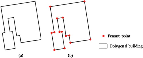
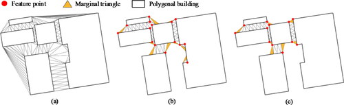
• Feature point. Vertex with an obvious right-angle turning tendency in the contour of the polygonal building. The geometric inflection in the contour of the polygonal building is evident; there is no continuous bending, and the fluctuation in the tangent angle change is small (Yan et al. 2016). Therefore, the corner cosine value ${\gamma }_{\mathit{turn}}$ of the vertex $p_i$ is used as the index for feature point recognition, and the calculation of ${\gamma }_{\mathit{turn}}$ is as follows:

(1) $${\gamma }_{\mathit{turn}}=\left|\frac{\stackrel{\rightharpoonup }{p_{i¯1}{p}_i}\cdot \stackrel{\rightharpoonup }{p_i{p}_{i+1}}}{\left|\stackrel{\rightharpoonup }{p_{i¯1}{p}_i}\right|.\left|\stackrel{\rightharpoonup }{p_i{p}_{i+1}}\right|}\right|$$(1)

In Equation 1(1) $${\gamma }_{\mathit{turn}}=\left|\frac{\stackrel{\rightharpoonup }{p_{i¯1}{p}_i}\cdot \stackrel{\rightharpoonup }{p_i{p}_{i+1}}}{\left|\stackrel{\rightharpoonup }{p_{i¯1}{p}_i}\right|.\left|\stackrel{\rightharpoonup }{p_i{p}_{i+1}}\right|}\right|$$(1) , $p_{i-1}$ is the leading vertex of $p_i,$ and $p_{i+1}$ is the trailing vertex of $p_i.$ When ${\gamma }_{\mathit{turn}}$ is less than the threshold ${\gamma }_{\mathit{thd}},$ it is considered that $p_i$ is a feature point. The feature points were extracted from the polygonal building shown in Figure 1(a), and the results are shown in Figure 1(b).

• Narrow obtuse triangle. An obtuse-angle triangle for which the ratio of its minimum bounding rectangle’s long and short edges is greater than or equal to the threshold $T_{\mathit{thd}}.$

• Visual conglutinate area. According to the Gestalt principle of proximity, polygonal buildings close to each other are more easily grouped (Li et al. 2004). The minimum visible distance was considered the distance index of group clustering, and the area between the polygonal buildings in the group is defined as the visual conglutinate area.

Figure 1. Extracting feature points of polygonal buildings. (a) Example of a polygonal building. (b) Extraction results.

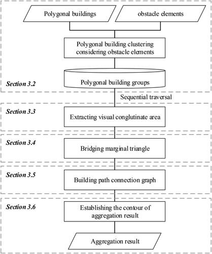
The schema for the polygonal building aggregation method, which considers obstacle elements and visual clarity, is illustrated in Figure 2. The main steps are described in detail in the following sections.

Figure 2. Schema of polygonal building aggregation.

3.2. Polygonal building clustering considering obstacle elements

The detection and determination of proximity relationships are prerequisites for polygonal building merging (Guo et al. 2016), which is usually based on the minimum visible distance $D_{\mathit{vis}}$ to determine whether there is visual conglutination between buildings as well as proximity relationships. Meanwhile, to avoid graphic rationality errors in the aggregation results that cross roads and rivers, it is necessary to use obstacle elements to partition polygonal buildings and cluster the partition results. We constructed a CDT using the contours of obstacle elements and the interpolated contours of polygonal buildings as constraints and classified the triangles into three types based on vertex association relationships (as shown in Figure 3(a)):

Figure 3. Polygonal building clustering considering obstacle elements. (a) Building CDT. (b) Result of deleting O-triangles and I-triangles. (c) Clustering results of polygonal buildings.

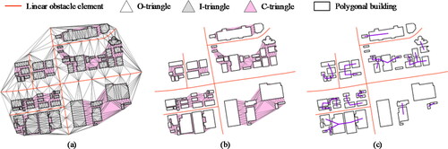
• O-triangle (outside triangle). The vertices of the triangles are associated with obstacle elements.

• I-triangle (inside triangle). The vertices of the triangles are associated with the same polygonal building and are located inside it.

• C-triangle (conglutinate triangle). Triangles in triangulation other than O-triangles and I-triangles.

As shown in Figure 3(b), deleting the O- and I-triangles in the CDT can prevent erroneous aggregation results that cross the obstacle elements.

The premise of clustering is to determine the distance between polygonal buildings, for which multiple methods are available. A calculation method for the visual distance between polygonal buildings based on the CDT was proposed. First, based on the number of triangles adjacent to the C-triangles, the triangles were further divided into four classes:

• Type I triangle. A triangle with 1 adjacent triangle.

• Type II triangle. A triangle with 2 adjacent triangles.

• Type III triangle. A triangle with 3 adjacent triangles.

• Type IV triangle. A triangle with 0 adjacent triangles, i.e. an isolated triangle.

Second, based on the different types of triangles, the calculation method for the triangle width was defined as follows: the type I triangle width is the length of the unconstrained edge, the type II triangle width is the shortest distance from the relative vertex of the constrained edge (open edge) to the constrained edge (open edge), and the type III and IV triangle widths are the average lengths of the three edges. The formula for calculating the distance between polygonal buildings, $P_m$ and $P_n,$ was as follows: (2) $$d_{m,n}={\sum }_{i=0}^k\mathit{Len}(tr{i}_i)/k$$(2) where $\mathit{Len}(tr{i}_i)$ is the width of a single C-triangle $tr{i}_i$ between $P_m$ and $P_n,$ and $k$ is the number of C-type triangles associated with $P_m$ and $P_n.$ If $d_{m,n}\le D_{\mathit{vis}}$ is used, there is a visual conglutination between $P_m$ and $P_n,$ and aggregation is required. After the visual distance calculation was completed, polygonal buildings with adjacent distances less than or equal to the $D_{\mathit{vis}}$ were grouped into the same cluster, and the clustering results were obtained (as shown in Figure 3(c)).

3.3. Extracting the visual conglutinate area

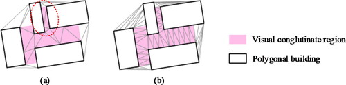
Extraction of the visual conglutinate area is a fundamental prerequisite for aggregation operations in polygonal building aggregation. The existing method for constructing a CDT with fixed step sizes cannot fully adapt to complex adjacent situations between polygonal buildings. It can easily generate many narrow obtuse triangles in the visual conglutinate area. Narrow obtuse triangles in the visual conglutinate area hurt the effectiveness of their range. As shown in Figure 4(a), there were two main reasons for the generation of narrow obtuse triangles: first, there was a considerable difference in the distance between polygonal buildings within the cluster, and second, the contours of adjacent polygonal buildings were not completely parallel.

Figure 4. Contour interpolation of polygonal buildings. (a) Fixed distance interpolation. (b) Adaptive distance interpolation.

To reduce the generation of narrow obtuse triangles in the visual conglutinate area and minimize the computational complexity of triangulation and subsequent processing, the construction of a DACDT was introduced. The minimum distance between the polygonal buildings within a cluster was denoted as $d_{\min },$ and the calculation method for the interpolation distance $L_d$ is shown in Equation (3)(3) $$L_d=\alpha \cdot d_{\min }+L_0$$(3) . (3) $$L_d=\alpha \cdot d_{\min }+L_0$$(3) where $\alpha$ is the interpolation distance adjustment parameter and $L_0$ is the initial interpolation distance. As shown in Figure 4(b), the number of narrow obtuse triangles in the visual conglutinate area was effectively reduced after the construction of the DACDT.

The DACDT filtering operation is important for obtaining an accurate and reasonable visual conglutinate area. Analysis shows a notable difference between the retained C-triangle group and the visual conglutinate area of cognition, mainly from the marginal part. Therefore, starting from the marginal triangles of the C-triangle group, deletion operations can be performed based on topological adjacency relationships and filtering rules to obtain a reasonable visual conglutinate area. The extraction process, shown in Figure 5, consisted of the following steps:

Figure 5. Flowchart for extracting the visual conglutinate area.

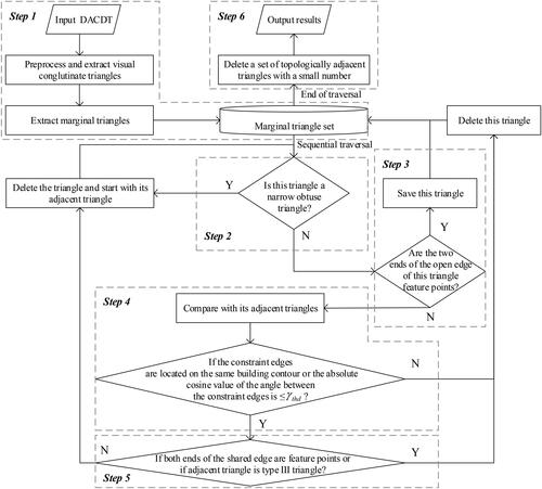
• Step 1. First, the constructed DACDT was pre-processed by deleting triangles with a width greater than or equal to $D_{\mathit{vis}}.$ Next, Type I triangles with two open edges, Type II triangles with one open edge, and Type IV triangles were deleted, and the set of marginal triangles in the DACDT was extracted according to the topological adjacency relationship. Finally, the marginal triangles were traversed in sequence before proceeding to step 2.

• Step 2. Whether a triangle was a narrow obtuse triangle was determined. If so, the triangle was deleted and step 2 was repeated, starting from the adjacent triangle; otherwise, we proceeded to step 3.

• Step 3. If both ends of the open edge of the triangle were feature points, the triangle was maintained and the next marginal triangle was traversed; otherwise, we proceeded to step 4.

• Step 4. The triangle was compared to its adjacent triangles, and if the constraint edges of both were located on the same contour of the polygonal building or if the absolute cosine of the angle between the constraint edges was less than or equal to ${\gamma }_{\mathit{thd}},$ we proceeded to step 5; otherwise, the triangle was deleted and the next marginal triangle was traversed.

• Step 5. If the vertices at both ends of the shared edge were feature points, or if the adjacent triangle was a Type III triangle, the triangle was deleted and the next edge triangle was traversed; otherwise, the triangle was deleted, and we returned to step 2 starting from its adjacent triangles until the set of edge triangles was traversed, at which time we proceeded to Step 6.

• Step 6. The set of topological adjacency triangles with a number less than or equal to $N_{\mathit{thd}}$ as well as the set of topological adjacency triangles with vertices located on the same contour of the polygonal building were deleted to avoid generating unreasonable visual conglutinate area extraction results.

The process of extracting the visual conglutinate area following the above steps is shown in Figure 6. The conglutinated regions of visual cognition were made relatively close by filtering and preserving the set of triangles.

Figure 6. Schematic diagrams of the visual conglutinate area extraction process. (a) DACDT construction. (b) Result of step 1 execution. (c) Result of visual conglutinate area extraction.

3.4. Bridging marginal triangles

The right-angled feature is the basic feature of artificial elements, such as polygonal buildings. The aggregation of polygonal buildings must consider the preservation of right-angled features and should be combined with locally shaped features between polygonal buildings for bridging. We designed bridging modes by using the marginal triangles of the visual conglutinate area as the basic bridging unit and considering the feature point constraints for bridging, we designed bridging modes.

• 0 feature points on the open edge. The open edge of the marginal triangle was not associated with the feature points of the polygonal building, and the requirement for maintaining the right-angled features was weak. Therefore, no right-angled bridging was performed (Figure 7).

• 1 feature point on the open edge. The open edge of the marginal triangle was associated with one feature point of the polygonal buildings, and the bridging modes were designed separately based on the relative positions of the feature points on the marginal triangle. When the feature point was located at the vertex opposite the constrained edge of the marginal triangle, regardless of the type of marginal triangle, it was directly perpendicular to the constrained edge from the feature point, intersecting with the constrained edge to obtain the foot point (Figures 8(a,b)). When the feature point was located on the constrained edge of the marginal triangle, it was necessary to reconstruct the marginal triangle using the adjacent point of the constrained edge relative to the vertex, and then draw a perpendicular line from the feature point to the reconstructed edge to obtain the foot point (Figure 8(c)).

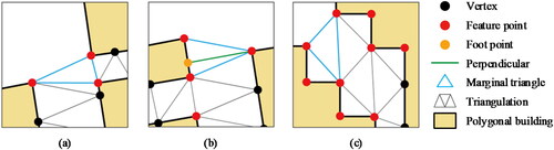
• 2 feature points are on the open edge, and the other is not a feature point. The open edge of the marginal triangle was associated with two feature points of the polygonal buildings, which were not located on the same constraint edge. First, we determined whether the absolute value of the cosine of the angle between the open edge of the marginal triangle and the constraint edge was less than or equal to ${\gamma }_{\mathit{thd}}:$ if it was less than ${\gamma }_{\mathit{thd}},$ no right-angled bridging was performed (Figure 9(a)); if it was greater than ${\gamma }_{\mathit{thd}},$ a perpendicular line was directly drawn from the feature point relative to the constraint edge towards the constraint edge, intersecting with the constraint edge to obtain the foot point (Figures 9(b,c)). Otherwise, the marginal triangle was reconstructed using the feature points relative to the constrained edge and its adjacent point with another feature point, and then a perpendicular line was drawn to the reconstructed edge to obtain the foot point (Figure 9(d)).

• 2 feature points are on the open edge, and the other is a feature point. If the three vertices of the marginal triangle are associated with different polygonal buildings (Figure 10(a)), it was necessary to delete the triangle, redefine the marginal triangle, and perform the aforementioned bridging modes based on the number of feature points on the open edge; otherwise, bridging was performed according to the bridging modes of the 2 feature point on the open edge and the other point is not a feature point (Figure 10(b)). In addition, when the contour of a polygonal building underwent twisting and turning, the marginal triangle did not contain a constrained edge. In this case, the bridging was the same as that in the mode of the 0 feature point (Figure 10(c)).

Figure 7. Bridging mode 1 with 0 feature points on the open edge.

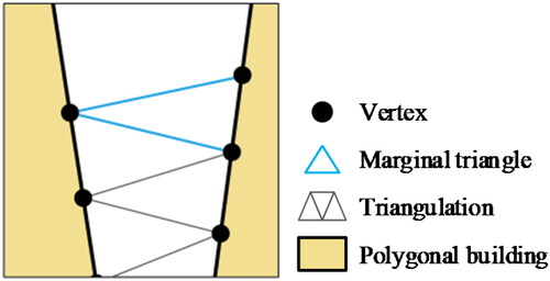
Figure 8. Bridging modes with 1 feature point on the open edge. (a) Bridging mode 2. (b) Bridging mode 3. (c) Bridging mode 4.

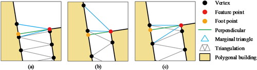
Figure 9. Bridging modes with 2 feature points are on the open edge and the other is not a feature point. (a) Bridging mode 5. (b) Bridging mode 6. (c) Bridging mode 7. (d) Bridging mode 8.

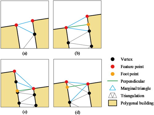
Figure 10. 2 feature points are on the open edge and the other is also a feature point. (a) The marginal triangle is associated with 3 polygonal buildings. (b) The marginal triangle is associated with 2 polygonal buildings and its bridging mode. (c) Special case.

3.5. Building the path connection graph

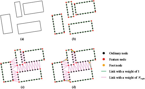
The data structure of a polygonal building is a serialized spatial coordinate point string. Serialization and orderliness are features of both data and spatial structures (Wang et al. 2005). Polygon aggregation involves breaking down multiple serialized spatial coordinate strings and then arranging, adding, or deleting coordinate points according to the set rules to generate new spatial coordinate strings. In this process, we introduced a graph theory to represent the coordinate points as nodes and the sequential connection relationships and association relationships within the filtered DACDT as links. This allows us to construct an undirected weighted path connection graph and perform polygonal building aggregation through a minimum loop search.

Taking the polygonal building to be aggregated as an example, as shown in Figure 11(a), the vertices of the polygonal buildings participating in the aggregation were first used as nodes, and the sequence connection relationship between the nodes was added as a link to $G.$ The link weight was set to 1, the node attribute was set to ordinary node, and the node’s attribute where the feature point was located was set to feature node (Figure 11(b)). Next, using the DACDT extracted from the visual conglutinate area, links were added between nodes in the $G,$ with the link weight set to $N_{\mathit{wight}}$ (The value that can be set as the sum of the number of vertices participating in the aggregation of polygonal buildings or a maximum value). The execution result is shown in Figure 11(c), where the foot points generated by the marginal triangle right-angled bridging were added to $G$ as foot nodes, and the links between the foot nodes and the three nodes of the corresponding edge triangle were added. The link weight was set to 1, and the $G$ was completed (Figure 11(d)).

Figure 11. Constructing a path connection graph. (a) Polygonal buildings to be aggregated. (b) Initial graph. (c) Intermediate graph. (d) Final graph.

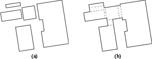
3.6. Establishing the contour of the aggregated result

Through the analysis of $G,$ it can be seen that nodes associated with triangulation have degrees >2, while nodes without triangulation have degrees of 2. Therefore, based on the degree of the nodes, ordinary nodes were categorized into two types: those with degree 2, denoted as unmarked ordinary nodes, and those with a degree >2, denoted as marked ordinary nodes. Combining $G$ and graph theory, the problem of establishing the contour of the polygonal building aggregation result was transformed into a problem of finding the minimum loop of the $G.$ By traversing the $G,$ the minimum loop set where unmarked ordinary nodes were located was obtained, and the corresponding coordinate points of the nodes were sequentially obtained to establish the contour of the aggregated result.

The steps for establishing the contour were as follows: initially, two adjacent and unmarked ordinary nodes $v_i$ and $v_j$ were considered and the link $e(v_i,v_j)$ between $v_i$ and $v_j$ in $G$ was temporarily deleted. Using the Dijkstra algorithm (Dijkstra 1959), the shortest path between $v_i$ and $v_j$ was identified, and the link $e(v_i,v_j)$ was supplemented to obtain the minimum loop. Subsequently, we marked the unmarked ordinary nodes on the minimum loop and repeated this step until there were no unmarked ordinary nodes in $G.$ Next, the nodes on the minimum loop were sequentially traversed to obtain the corresponding coordinate points for each node in order. A closed spatial coordinate point string was then obtained, the outer contour and open land boundary of the aggregation result were determined according to the spatial relationship, and the island with an area less than the threshold $A_{\mathit{thd}}$ was deleted to obtain the final aggregation result (Figure 12).

Figure 12. (a) Polygonal buildings to be aggregated. (b) Aggregation result.

4. Results and discussion

4.1. Experimental design and setting

To verify the superiority of the proposed method, it was implemented using Python in ArcGIS Pro 2.5 desktop software. The experimental data were selected from the OpenStreetMap (OSM) polygonal building data of several blocks in the Nanjing urban area. The chosen area was ∼2.5 km² and contained 888 building polygons. The OSM road was selected as an obstacle element. After repeated experimental comparisons and analyses, set $T_{\mathit{thd}}\text{=}3,$ $\alpha \text{=}0.1,$ $L_0\text{=}0.1mm,$ $N_0=1,$ and ${\gamma }_{\mathit{thd}}=0.259;$ The $D_{\mathit{vis}}=0.4mm$ setting referred to Wang et al. 2021; Set $A_{\mathit{thd}}=D_{\mathit{vis}}{}^2,$ which can be set according to different needs. The specific parameters and corresponding threshold settings are shown in Table 1.

Table 1. Experimental parameter settings.

Symbol	Description	Value
$T_{\mathit{thd}}$	Narrow obtuse triangle judgment threshold	3
$D_{\mathit{vis}}$	Minimum visible distance	0.4 mm
$\alpha$	Interpolation distance adjustment threshold	0.1
$L_0$	Initial interpolation distance	0.1 mm
$N_0$	Constant for group deletion	1
${\gamma }_{\mathit{thd}}$	Threshold for feature point extraction	0.259
$A_{\mathit{thd}}$	Area threshold for island preservation	0.16 mm^2

We selected the Esri method (https://pro.arcgis.com/zh-cn/pro-app/latest/tool-reference/cartography/aggregate-polygons.htm), Guo (Guo et al. 2016) and Li methods (Li et al. 2023) for comparison with our proposed method. To avoid drawing unwarranted comparison conclusions arising from varying parameters, we set the target scale of aggregation at 1:50,000. All methods used the same island preservation threshold and minimum visible distance, and all used roads as obstacle elements for polygonal building clustering (in the ArcGIS Pro 2.5 polygon aggregation tool, the orthogonal shape was retained and roads were added as obstacle elements).

4.2. Effectiveness evaluation

Figure 13 illustrates the aggregate results. The changes in number, area, islands, and ratio of right-angled vertices achieved by the different methods were counted, where the right-angled ratio refers to the ratio of the number of right-angled vertices (defined as the angle between the vertex and its front and back vertices within the interval [85°, 95°]) to the total number of vertices in the polygonal buildings. To avoid differences in the number of vertices in different aggregation results caused by different interpolation methods during CDT construction, the Douglas-Peucker algorithm (Douglas and Peucker 1973) with a small threshold was used to dilute the vertices in the aggregation results; the dilution threshold was set to 0.1 m of a field distance. Table 2 presents the statistical results.

Figure 13. Comparison of polygonal building aggregation results using different methods. (a) The Esri method. (b) The Guo method. (c) The Li method. (d) Our proposed method.

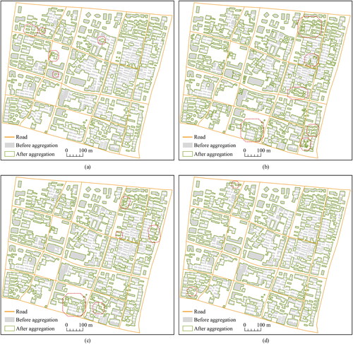
Table 2. Quantitative statistics of the aggregation results were achieved using different methods.

Method	Number of polygonal buildings	Quantity change rate (%)	Total area (m^2)	Area change rate (%)	Number of islands	Total island area (m^2)	Number of right-angled vertices	Number of right-angled vertices on the island	ratio of right-angled vertices (%)
Experimental data	888	–	756,333.2	–	0	0	4504	0	93.35
Esri method	114	87.16	1,132,028.5	49.67	28	43,202.4	2607	162	79.07
Guo method	68	92.34	1,086,892.6	43.71	112	151,397.0	3616	1008	73.69
Li method	61	93.13	1,125,532.5	48.81	103	180,833.2	2901	881	70.62
Proposed method	80	90.99	1,133,347.3	49.85	53	82,539.3	2772	411	73.16

Upon analyzing the aggregation results, we observed that all four methods effectively reduced the number of polygonal buildings through aggregation, achieving a visual conglutinate polygonal building aggregation. When comparing the changes in the number, area, and islands of polygonal buildings before and after aggregation, we observed that the Guo and Li methods outperformed others in terms of quantity reduction, area retention, and island expression; however, some details remained unclear. As shown in the dashed boxed areas of Figures 13(b,c), the shape of the islands was complex and densely distributed, increasing visual congestion and ambiguity; meanwhile, when the visual conglutinate area was aggregated, there were many unreasonably narrow bridging polygons, which hurt the accurate expression of the aggregation results. In comparison, our proposed method and the Esri method retained a relatively small number of islands, and the constructed bridge polygons were close to the visual conglutinate area. However, the regularity of the island achieved by the Esri method requires improvement, and some visually conglutinate polygonal buildings were not aggregated (as shown in the dashed boxed area in Figure 13(a)).

We also compared the preservation effects of the right-angled and locally shaped features. The aggregation results of the Guo and Li methods had more right-angled vertices due to the large number of reserved islands. Notably, there were also differences between the two methods: the Guo method performed bridge polygon right-angled processing, increasing the number of right-angled vertices on the outer contour of the aggregation result without considering the locally shaped features between polygonal buildings, while the Li method took into account the spatial structure relationship in the treatment strategy of the inclined bridge polygon, which reduced the number of right-angled vertices on the outer contour of the aggregation result. The Esri method was similar to the Guo method in terms of the process of right-angled bridging; therefore, the proportion of right-angled vertices was relatively high.

The proposed method combined feature point constraints to perform targeted bridging processing on marginal triangles, which considered the locally shaped features on both sides of the bridging polygon and maintained the right-angled features, achieving good aggregation. It should be noted that there is still a gap between the processing results of the proposed method and manual processing results when dealing with complex bridging situations (as shown in the dashed boxed area of Figure 13(a)). However, compared to the results of the other three methods, this method provided more advantages. Unreasonable details can be eliminated using the building-simplification method.

4.3. Clarity evaluation

The main purpose of polygonal building aggregation is to solve the problem of visual conglutination caused by downscaling and to meet the requirement of clear visibility at the target scale. Therefore, it is important to determine the clarity of the aggregation results. Indices of degree of visual conglutination (DVCon) and degree of visual complexity (DVCom) have been proposed to evaluate the clarity of aggregation results quantitatively. The aggregation of polygonal buildings can be perceived as a reduction in the visual conglutination area: the smaller the area of the visual conglutination on the map, the clearer the aggregation result. DVCon was defined as the ratio of the visual conglutinate area to the map area and was calculated using Equation (4)(4) $$\text{DVCon=}\frac{S_{\mathit{Con}}}{S}$$(4) . (4) $$\text{DVCon=}\frac{S_{\mathit{Con}}}{S}$$(4) where $S_{\mathit{Con}}$ is the visual conglutinate area, and $S$ is the map area. We used the step described in Section 3.3 to extract the visual conglutinate area before and after the aggregation of experimental data using four aggregation methods (Figures 14 and 15, respectively) and calculated the DVCon (Table 3). The analysis showed that the visual conglutinate area at the target scale can be significantly eliminated through aggregation operation, thereby improving visual clarity. Compared to the other methods, the DVCon of the aggregation results achieved with our proposed method was smaller, indicating higher clarity.

Figure 14. Visual conglutinate area extraction results from experimental data.

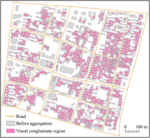
Figure 15. Visual conglutinate area extraction results based on the aggregation results of different methods. (a) The Esri method. (b) The Guo method. (c) The Li method. (d) Our proposed method.

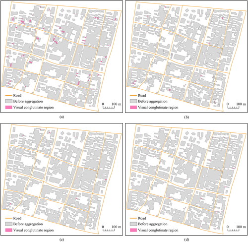
Table 3. Calculation of degree of visual conglutination.

Methods	The area of visual conglutinate area (m^2)	DVCon (%)
Experimental data	386,926.1	15.478
Esri method	19,780.0	0.791
Guo method	3288.0	0.131
Li method	1691.2	0.067
Proposed method	1267.2	0.051

Bold indicates the minimum value of each column.

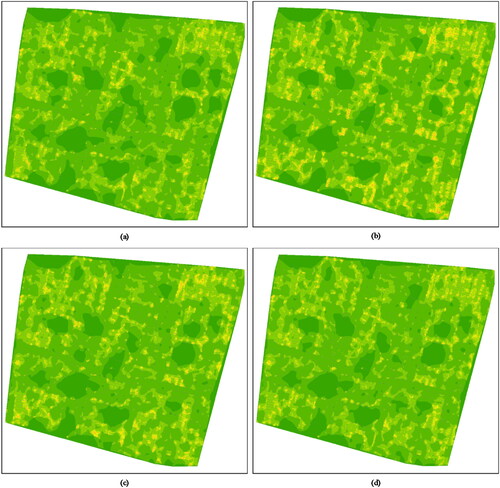
DVCon can evaluate visual clarity on the whole quantitatively; however, it does not consider the contour clarity of polygonal buildings. Therefore, we measured the complexity of line elements (Wei et al. 2022) to generate a complex contour field for a polygonal building (Figures 16 and 17) to quantitatively evaluate DVCom in the experimental area. The analysis showed that the DVCom of the experimental data was significantly high, indicating low clarity. Areas with higher DVCom were mostly concentrated in visual conglutinate areas, complex-shaped islands, narrow bridge polygons, continuous turning points of contours, and areas where the island was close to the outer contour of the polygonal building. The Esri method achieved a higher DVCom, mainly concentrated in the conglutinate visual area and continuous turning points of contours. The Guo and Li methods also achieved higher DVCom values, concentrated in the latter four areas, with relatively low clarity. The higher DVCom of the proposed method was mainly concentrated in the last two areas.

Figure 16. The complex field of polygonal buildings before aggregation.

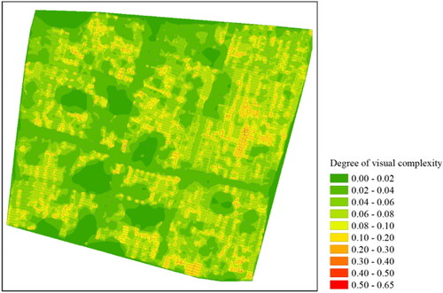
Figure 17. The complex field of polygonal buildings after aggregation. (a) The Esri method. (b) The Guo method. (c) The Li method. (d) Our proposed method.

Table 4 presents a further statistical analysis of the DVCom of the different methods. Although the average and standard deviation of the DVCom obtained from the Guo and Li methods were smaller than those of the experimental data, the maximum value of DVCom increased year-on-year, indicating that the clarity of the local areas in the aggregation results was lower than previously, leading to local abnormalities. The Esri method had the lowest average DVCom among the four methods, and the standard deviation of DVCom was the same as that of our proposed method; however, the maximum value of DVCom did not decrease significantly. In comparison, our proposed method significantly reduced the maximum DVCom value, close to the average DVCom value achieved by the Esri method, indicating higher clarity in local areas.

Table 4. Statistical results of degree of visual complexity.

Methods	Minimum value	Maximum value	Average value	Standard deviation
Experimental data	0.002	0.474	0.053	0.029
Esri method	0.002	0.438	0.035	0.017
Guo method	0.002	0.578	0.041	0.023
Li method	0.002	0.625	0.037	0.0194
Proposed method	0.002	0.288	0.036	0.017

Bold indicates the minimum value of each column.

5. Conclusions

This study proposed a polygon aggregation method for buildings that considers obstacle elements and visual clarity. The proposed method includes three main progressive processes: clustering polygonal buildings, extracting visual conglutinate areas, and establishing the contour of the aggregation results. By selecting polygonal building data from Nanjing for comparative experiments and analyses, the following conclusions were drawn:

• The proposed method can effectively handle the aggregation of polygonal buildings. By introducing obstacle elements for clustering and neighbouring relationships for filtering, a visual conglutinate area that conforms to cognition can be obtained

• Bridging modes have been designed to balance the preservation of right-angled and locally shaped features while considering the ability to reduce the quantity, maintain area, and express islands.

• By introducing the degree of visual conglutination to evaluate the overall clarity of the aggregation results and the degree of visual complexity to evaluate the local area clarity of the aggregation results, the proposed method presented more advantages in improving the clarity of the aggregation results compared with the other three methods tested.

Thus, the proposed method can be applied to the mapping and multiscale expression of polygonal buildings in urban areas. However, the effectiveness of aggregation in rural areas with hash distribution requires further research. In the future, it will be necessary to study the constraint and guiding effect of visual clarity on the aggregation process. In addition to preserving right-angled and local shape features, it will also be necessary to introduce other geographical features to improve the geographical adaptability of the proposed method.

Acknowledgements

We are grateful to the editor and the anonymous referees for their valuable comments and suggestions.

Disclosure statement

No potential conflict of interest was reported by the author(s).

Data availability statement

Data and code are available from the corresponding author by request.

Additional information

Funding

This work was supported by the National Natural Science Foundation of China under Grant [numbers 42101454, 42101455] and the Fund Project of ZhongYuan Scholar of Henan Province of China under Grant [number 202101510001].

References

- Ai T, Zhang X, Zhou Q, Yang M. 2015. A vector field model to handle the displacement of multiple conflicts in building generalization. Int J Geogr Inform Sci. 29(8):1310–1331. doi: 10.1080/13658816.2015.1019886.
- Burghardt D, Cecconi A. 2007. Mesh simplification for building typification. Int J Geogr Inform Sci. 21(3):283–298. doi: 10.1080/13658810600912323.
- Cetinkaya S, Basaraner M, Burghardt D. 2015. Proximity-based grouping of buildings in urban blocks: a comparison of four algorithms. Geocarto Int. 30(6):618–632. doi: 10.1080/10106049.2014.925002.
- Dijkstra EW. 1959. A note on two problems in connexion with graphs. Numerische Mathematik. 1(1):269-271. doi: 10.1007/BF01386390.
- Douglas DH, Peucker TK. 1973. Algorithms for the reduction of the number of points required to represent a digitized line or its caricature. Cartographica. 10(2):112–122. doi: 10.3138/FM57-6770-U75U-7727.
- Du S, Luo L, Cao K, Shu M. 2016. Extracting building patterns with multilevel graph partition and building grouping. ISPRS J Photogramm Remote Sens. 122:81–96. doi: 10.1016/j.isprsjprs.2016.10.001.
- Du J, Wu F, Xing R, Li C, Li J. 2022. Trial and comparison of some encoder-decoder based deep learning models for automated generalization of buildings. Geom Inform Sci Wuhan Univ. 47(7):1052–1062.
- Feng Y, Thiemann F, Sester M. 2019. Learning cartographic building generalization with deep convolutional neural networks. ISPRS Int J Geoinform. 8(6):258. doi: 10.3390/ijgi8060258.
- Gong X, Wu F. 2018. A typification method for linear pattern in urban building generalisation. Geocarto Int. 33(2):189–207. doi: 10.1080/10106049.2016.1240718.
- Guercke R, Götzelmann T, Brenner C, Sester M. 2011. Aggregation of LoD 1 building models as an optimization problem. ISPRS J Photogramm Remote Sens. 66(2):209–222. doi: 10.1016/j.isprsjprs.2010.10.006.
- Guo P, Li C, Yin Y. 2016. Classification and filtering of constrained Delaunay triangulation for automated building aggregation. Acta Geodaet Cartogr Sin. 45(8):1001–1007.
- Guo Q, Li J, Cao Y, Wang Y, Liu J, Zheng C. 2021. Automatic aggregation of building footprint polygons. Geom Inform Sci Wuhan Univ. 46(1):12–18.
- Guo R, Ai T. 2000. Simplification and aggregation of building polygon in automatic map generalization. J Wuhan Tech Univ Surv Mapp. 25(1):25–30.
- He X, Zhang X, Xin Q. 2018. Recognition of building group patterns in topographic maps based on graph partitioning and random forest. ISPRS J Photogramm Remote Sens. 136:26–40. doi: 10.1016/j.isprsjprs.2017.12.001.
- He X, Zhang X, Yang J. 2018. Progressive amalgamation of building clusters for map generalization based on scaling subgroups. ISPRS Int J Geoinform. 7(3):116. doi: 10.3390/ijgi7030116.
- Li A, Zhai R, Yin J, Zhu L, Qi L. 2023. Automatic aggregation of building considering the spatial structure. Geom Inform Sci Wuhan Univ. doi: 10.13203/j.whugis20210731.
- Li C, Wu W, Yin Y, Wu P, Wu Z. 2022. A multi‐scale partitioning and aggregation method for large volumes of buildings considering road networks association constraints. Trans GIS. 26(2):779–798. doi: 10.1111/tgis.12885.
- Li C, Yin Y, Wu P, Wu W. 2021. An area merging method in map generalization considering typical characteristics of structured geographic objects. Cartogr Geogr Inform Sci. 48(3):210–224. doi: 10.1080/15230406.2020.1863862.
- Li Z. 2006. Algorithmic foundation of multi-scale spatial representation. Boca Raton: CRC Press.
- Li Z, Yan H, Ai T, Chen J. 2004. Automated building generalization based on urban morphology and Gestalt theory. Int J Geogr Inform Sci. 18(5):513–534. doi: 10.1080/13658810410001702021.
- Liu Q, Deng M, Shi Y, Wang J. 2012. A density-based spatial clustering algorithm considering both spatial proximity and attribute similarity. Comput Geosci. 46:296–309. doi: 10.1016/j.cageo.2011.12.017.
- Ma J, Zhou Z, Zhang F. 2023. Combined building simplification approach considering multi-feature constraints. J Geo-Inform Sci. 25(2):277–287.
- Pilehforooshha P, Karimi M. 2020. A local adaptive density-based algorithm for clustering polygonal buildings in urban block polygons. Geocarto Int. 35(2):141–167. doi: 10.1080/10106049.2018.1508313.
- Qian H, Wu F, Tan X, Deng H. 2005. The algorithm for merging city buildings based on ABTM. J Image Graph. 10(10):1224–1233.
- Regnauld N, Revell P. 2007. Automatic amalgamation of buildings for producing ordnance survey® 1: 50 000 scale maps. Cartogr J. 44(3):239–250. doi: 10.1179/000870407X241782.
- Sester M, Feng Y, Thiemann F. 2018. Building generalization using deep learning. Int Arch Photogramm Remote Sens Spatial Inf Sci. XLII-442:565–572. doi: 10.5194/isprs-archives-XLII-4-565-2018.
- Shen Y, Ai T, Li W, Yang M, Feng Y. 2019. A polygon aggregation method with global feature preservation using superpixel segmentation. Comput Environ Urban Syst. 75:117–131. doi: 10.1016/j.compenvurbsys.2019.01.009.
- Shen Y, Li J, Wang Z, Zhao R, Wang L. 2022. A raster-based typification method for multiscale visualization of building features considering distribution patterns. Int J Digital Earth. 15(1):249–275. doi: 10.1080/17538947.2021.2023668.
- Wang H, Wu F, Wang B, Deng H. 2005. The algorithm for aggregation of polygon applied to automatic map generalization. Eng Surv Mapp. 14(5):15–18.
- Wang W, Du S, Guo Z, Luo L. 2015. Polygonal clustering analysis using multilevel graph-partition. Trans GIS. 19(5):716–736. doi: 10.1111/tgis.12124.
- Wang Y, Luo A, Wang H, Cao Y, Liu J. 2021. A method of polygon aggregation for complex buildings based on shortest adjacent lines. Acta Geodaet Cartogr Sin. 50(12):1671–1682.
- Wei H, Zhang L, Tang L, Dong J, Li G, Yuan H. 2022. Complexity measurement of line element on nautical chart considering local difference. Acta Geodaet Cartogr Sin. 51(9):1959.
- Wei Z, Guo Q, Wang L, Yan F. 2018. On the spatial distribution of buildings for map generalization. Cartogr Geogr Inform Sci. 45(6):539–555. doi: 10.1080/15230406.2018.1433068.
- Wu L, Xie Z, Ye Z. 2009. A building polygon generalization algorithm under the road constraint. Geogr Geo-Inform Sci. 27(6):111–112.
- Yan H, Weibel R, Yang B. 2008. A multi-parameter approach to automated building grouping and generalization. Geoinformatica. 12(1):73–89. doi: 10.1007/s10707-007-0020-5.
- Yan H, Ying S, Li L. 2008. An approach for automated building grouping and generalization considering multiple parameters. Geom Inform Sci Wuhan Univ. 33(1):51–54.
- Yan X, Ai T, Yang M. 2016. A simplification of residential feature by the shape cognition and template matching method. Acta Geodaet Cartogr Sin. 45(7):874.
- Yu W, Zhou Q, Zhao R. 2021. A heuristic approach to the generalization of complex building groups in urban villages. Geocarto Int. 36(2):155–179. doi: 10.1080/10106049.2019.1590463.