Mapping high marsh and salt pannes/flats along the northern Gulf of Mexico coast

Abstract

Coastal wetlands are predicted to undergo extensive transformation due to climate and land use change. Baseline maps of coastal wetlands can be used to help assess changes. Found in the upper portion of the estuarine zone, high marsh and salt pannes/flats provide ecosystem goods and services and are particularly important to fish and wildlife. We developed the first map of high marsh and salt pannes/flats along the northern Gulf of Mexico using regional models that included spectral indices related to greenness and wetness from optical satellite imagery, elevation data, irregularly flooded wetland probability information, and synthetic aperture radar backscatter. We found the greatest relative coverage of high marsh along the Texas coast (30% to 65%) and the Florida Panhandle (40%), whereas the greatest relative coverage of salt pannes/flats was along the lower Texas coast (74%) and the middle Texas coast (15%). As part of this effort, we also developed a map that highlighted irregularly flooded wetlands dominated by Juncus roemerianus (black needlerush) for part of the study area. Both maps had an overall accuracy of around 80%. Our results advance the understanding of estuarine marsh zonation and provide a baseline for assessing future transformations.

HIGHLIGHTS

• This is the first map of high marsh and salt pannes/flats along the northern Gulf of Mexico and provides a baseline for understanding transformations predicted to occur with climate change.

• Due to high elevation uncertainty in wetlands, we used a map of irregularly flooded wetland probability that was created using elevation error assumptions.

• Irregularly flooded wetland probability, synthetic aperture radar backscatter, and spectral indices related to greenness and wetness were important predictor variables.

• Differences in wetland zonation and species composition along the study area led to variation in models by region.

• The framework presented here could be adapted to other areas.

Keywords:

• Random forest
• coastal wetlands
• synthetic aperture radar
• data fusion
• elevation

1. Introduction

Coastal wetlands provide numerous ecosystem goods and services (Barbier 2011), including supporting important fish and wildlife habitat (Sievers et al. 2019; Haverland et al. 2021), improving water quality (Mitsch and Wang 2000), storing carbon (Morris et al. 2012), protecting coastlines and coastal communities from flooding (Möller et al. 2014), and providing recreational opportunities (Bergstrom et al. 1990). The distribution and characteristics of coastal wetlands are regulated by broad ecological drivers, such as climate and climate change (Gabler et al. 2017; Reed et al. 2022), and local stressors that include tidal range (Kirwan and Guntenspergen 2010), relative sea-level rise (Sweet et al. 2022), precipitation (Osland et al. 2014; Stagg et al. 2020; Wang et al. 2022), sediment availability (Morris et al. 2002), winter temperatures (Osland et al. 2021), extreme storm frequency (Cahoon 2006; Thorne et al. 2022), and land use practices (Mitsch and Gosselink 2007; Novoa et al. 2020). The dynamic nature of coastal wetland systems coupled with their importance underscores the need to map their current distribution and structure so that resource managers and researchers can document the localized threats posed by climate change.

While better information on the extent of coastal wetlands is needed, maps that delineate coastal wetland vegetation zonation based on broad classes of flooding and salinity tolerance, such as fresh, intermediate, brackish, and saline (Enwright et al. 2015), are generally lacking. Such maps can provide additional information to enhance management of these systems including improved monitoring of change within coastal wetlands for floral coverage and species distribution and improving linkages between faunal habitat availability and species distribution (Ennen et al. 2019; Krainyk et al. 2019; Tolliver et al. 2019). Of particular interest along the Gulf of Mexico are high marsh and salt pannes/flats, which occupy a subset of coastal wetlands. High marsh and salt pannes/flats are found in the upper portion of the estuarine zone and are irregularly flooded (i.e. less than daily) by shallow polyhaline waters (i.e. salinity between 18 and 30 parts per thousand) associated with lunar tides, perigean spring tides, wind-induced water level fluctuations, and storms (USNVC 2022). Along the Gulf of Mexico coast of the United States, high marsh systems are typically dominated by Spartina patens (saltmeadow cordgrass), Spartina spartinae (Gulf cordgrass), and Spartina bakeri (marsh grass) (USNVC 2022). In this region, salt pannes are small depressions within salt marshes where hypersaline conditions develop through the evaporation of polyhaline waters and often have succulent marsh species (Salicornia spp. and Batis spp.) and algal mats (USNVC 2022). Salt flats have similar vegetation characteristics to salt pannes, but they are often located within hypersaline estuaries (e.g. Laguna Madre, Texas; USNVC 2022).

High marsh and salt pannes/flats provide important breeding habitat for bird species of conservation concern like Wilson’s Plover (Charadrius wilsonia), Seaside Sparrow (Ammodramus maritimus), and the federally threatened Eastern Black Rail (Laterallus jamaicensis jamaicensis; Haverland 2019, Haverland et al. 2021; Stevens et al. 2022). These systems also provide habitat for species like Yellow Rail (Coturnicops noveboracensis; Morris et al. 2017; Butler et al. 2022) and Mottled Duck (Anas fulvigula; Krainyk et al. 2019; Moon et al. 2021), which are targets for conservation and management along coastal areas, and numerous fish and crustaceans (Boesch and Turner 1984; MacKenzie and Dionne 2008). Land managers need baseline information on the distribution and extent of high marsh and salt pannes/flats given the projected increases in inundation predicted to occur over the next several decades with accelerated sea-level rise (Sweet et al. 2022). Increases in the frequency of inundation are predicted to have a high magnitude along the northern Gulf of Mexico where elevated inundation may occur within the next decade (Thompson et al. 2021). Increased inundation associated with sea-level rise may eliminate high marsh in many areas where it currently occurs and will require a potentially rapid upslope migration of these irregularly flooded wetlands for them to survive in the future (Osland et al. 2022).

Although multiple national mapping efforts exist for coastal wetlands, none of these delineate high marsh and salt panne/flats subsystems. For example, these subsystems are not explicitly delineated in national mapping efforts, such as the United States Fish and Wildlife Service’s National Wetlands Inventory (NWI; U.S. Fish and Wildlife Service 2022) or the National Oceanic and Atmospheric Administration’s (NOAA) Coastal Change Analysis Program (C-CAP; NOAA 2016). Instead, maps of high marsh and salt pannes/flats have been developed as stand-alone efforts at the regional or local level. Correll et al. (2018) developed a map of wetland types that included high marsh and salt pannes from Maine to the eastern shore Chesapeake Bay in Maryland. The map was developed using a random forest classifier that used 3-m elevation data, elevation data relative to various tidal datums, raw digital numbers from 1-m color-infrared aerial imagery, a wetness index, a greenness index, and information from a principal component analysis of the 4-band imagery. Allen (2017) mapped high marsh, salt pannes, and other marsh types for Georgia and North Carolina in 2014 using Landsat 8 imagery. Their approach also used elevation data, synthetic aperture radar (SAR), and the normalised difference index composite approach introduced by Rogers and Kearney (2004). The maps were created using an object-based image analysis using mean shift segmentation. Allen (2019) expanded on this approach by incorporating the normalised difference index composite along with relative tidal elevation information to map high marsh, salt pannes, and other marsh types from Mobile Bay in Alabama to Florida using object-based image analysis and a support vector machine classifier. High marsh and salt pannes/flats have also been mapped at the state and local levels. For example, these subsystems were mapped for Texas Ecological Mapping Systems (Elliott et al. 2014) and for the Grand Bay National Estuarine Research Reserve (Pitchford 2019). Despite these helpful products, there is currently no single map depicting high marsh and salt pannes/flats across the northern Gulf of Mexico coast.

Our objective was to develop a regional map of high marsh and salt pannes/flats for the United States portion of the northern Gulf of Mexico coast. We built upon work of Correll et al. (2018) and Allen (2019) by using SAR imagery, spectral indices from multispectral optical satellite imagery, and elevation information to map high marsh and salt pannes/flats. Given the error in elevation datasets in coastal wetlands coupled with spatially dynamic tidal water levels, we utilized an elevation-based map depicting irregularly flooded wetland probability based upon uncertainty information and Monte Carlo simulations (Enwright et al. 2023b). Specifically, this layer provides a mask for where we may expect to find high marsh and salt pannes/flats based on elevation while also accounting for common elevation error issues in wetlands.

2. Methods

2.1. Study area

The study area spanned five states along the northern Gulf of Mexico (Figure 1) and included coastal wetlands that were located within a generalized 5-m elevation contour (relative to the North American Vertical Datum of 1988 [NAVD88]) that was created from 1/3 arcsecond DEMs (10 m) from the USGS 3D Elevation Program (3DEP) (USGS 2020).

Figure 1. Study area along the northern Gulf of Mexico representing high marsh mapping regions (a-d) and associated watersheds. Pane e shows the full study area and the location of each region. * regions where high marsh and salt panne/flat classification models were developed. ^ regions where study-specific field data were collected. Watershed inset map and number (e.g. a1, a2, etc.). This figure is modified from Enwright et al. (2023b).

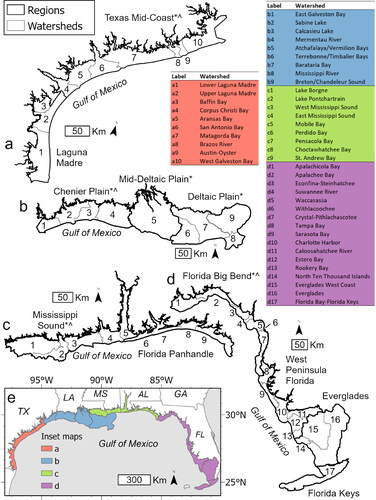
The southeastern region of the United States has a gently sloping coastal plain that includes a large portion of the coastal wetlands located in the conterminous United States (Greenberg et al. 2006). The northern Gulf of Mexico is a microtidal system with a tidal amplitude from 0.5–1 m (NOAA 2019a) and a high proportion of brackish wetlands (Greenberg et al. 2006). Differences in geomorphology, climate, and management of coastal lands across the northern Gulf of Mexico leads to important variations in coastal wetland zonation and species composition (Gabler et al. 2017). Enwright et al. (2023b) provides more insights concerning the features that change regionally within the study area. To account for the documented regional variation, we developed maps for 11 geographic regions along the northern Gulf of Mexico (Figure 1) that were based on watershed boundaries (Dale et al. 2022). Regions included: (1) Laguna Madre; (2) Texas Mid-Coast; (3) Chenier Plain; (4) Mid-Deltaic Plain; (5) Deltaic Plain; (6) Mississippi Sound; (7) Florida Panhandle; (8) Florida Big Bend; (9) West Peninsula Florida; (10) Everglades; and (11) Florida Keys (Figure 1).

2.2. Coastal wetland mask

Because watersheds within the study area included non-wetland cover types, we used the coastal wetland mask, described in Enwright et al. (2023b). Briefly, the coastal wetland mask was developed using a combination of NOAA’s 2016 Coastal Change Analysis Program (C-CAP) 30-m dataset (NOAA 2016) and 10-m BETA C-CAP land cover dataset (NOAA 2019b). The mask was based on four land cover classes: (1) estuarine emergent marsh; (2) estuarine scrub/shrub wetlands; (3) estuarine forested wetlands; and (4) unconsolidated shore (i.e. ‘non-vegetated areas subject to inundation and redistribution due to the action of water’; NOAA 2019b). In addition to estuarine wetlands, we also included adjacent palustrine emergent marsh and palustrine scrub/shrub wetlands in this study to account for possible classification errors and ensure a comprehensive mapping extent (i.e. reduce omission error) for subsequent high marsh classification. Unless noted otherwise, spatial data analyses were conducted using Esri ArcGIS Pro 2.9 (Redlands, California, USA). Table 1 highlights all data used in this study.

Table 1. Data sources used for mapping high marsh and salt pannes/flats along the northern Gulf of Mexico, USA.

Data type	Source	Spatial resolution (m)	Use
Land cover data	2015 habitat map for Grand Bay National Estuarine Research Reserve (Pitchford 2019)	NA (vector)	Ancillary ground reference data points for high marsh and salt pannes/flats
	National Oceanographic and Atmospheric Administration’s (NOAA) 2016 Coastal Change Analysis Program (C-CAP) land cover (NOAA 2016)	30	Coastal wetland mask development; Photointerpretation for ancillary ground reference data collection for ground reference points for water, barren, and salt pannes/flats for training and testing data
	NOAA 10-m BETA C-CAP land cover dataset (NOAA 2019b)	10
	Florida Statewide Land Use Land Cover (FDEP 2017)	NA (vector)	Map refinement in South Florida (see supplemental material)
Elevation-based data	Elevation relative to mean higher high water from best available digital elevation models (Enwright et al. 2023a,b)	10	Predictor variable
	Irregularly flooded wetland probability from best available digital elevation models (Enwright et al. 2023a,b)	10
Optical satellite imagery	Sentinel-2 multispectral surface reflectance imagery (Copernicus Sentinel data 2019–2020 2021)	10–20	Predictor variable
Radar satellite imagery	Sentinel-1 C-band synthetic aperture radar data (Copernicus Sentinel data 2020 2021)	10	Predictor variable
Vegetation data	Various sources (see Table 2)	NA (various plot-level)	In situ ground reference for training and testing data

2.3. Mapping high marsh and salt pannes

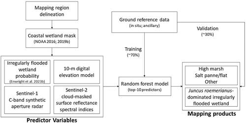
Figure 2 depicts the process used to develop the high marsh and salt pannes/flats map. The sections below cover the general methods used for this study while additional details are described in the supplemental material.

Figure 2. Overview of the approach used for mapping high marsh and salt pannes/flats along the northern Gulf of Mexico coast, USA.

Similar to Correll et al. (2018), our goal was to produce a map of high marsh and other subsystems defined by the Saltmarsh Habitat and Avian Research Program (SHARP; https://tidalmarshbirds.org/), which include: (1) high marsh; (2) low marsh; (3) salt pools/pannes; (4) terrestrial border; (5) Phragmites; (6) mudflat; (7) open water; and (8) upland. We added an additional class called barren that featured sandy areas that did not fall into the SHARP classification. However, upon visual inspection of initial model results, we decided to focus on mapping high marsh and salt pannes/flats instead of the broader SHARP classes. Our rationale for this decision was largely due to ambiguity in the definition and usage of the terrestrial border class, which was defined as an ‘area infrequently flooded by storm and spring tides and can include areas of marsh with fresh/brackish water due to a high water table and/or runoff from impervious surfaces’ by Correll et al. (2018). As defined, these wetlands appear to be those located along the marsh/upland transition; however, for our initial maps the terrestrial border class included expansive areas in riparian corridors in our initial results for the Gulf of Mexico.

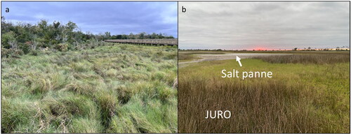
Vegetative characteristics for high marsh have been described for small portions of the Gulf of Mexico but plant species composition differs (Wieland 2007; Rasser et al. 2013) across the northern Gulf of Mexico. Although species composition differs, all descriptions focus on coastal marshes where infrequent tidal flooding combined with persistent evaporation cause salts to accumulate, which in turn reduces species richness and cover. To account for differences in species composition, we used two groups from the United States National Vegetation Classification System (USNVC) to define high marsh and salt pannes/flats, which both fell within the irregularly flooded zone (USNVC 2022). We used G121 Spartina patens—Iva frutescens High Salt Marsh Group as the definition for high marsh and USNVC G123 Salicornia spp.—Sarcocornia spp.—Spartina spartinae Tidal Flat & Panne Group for the definition of salt pannes/flats. Examples of high marsh and salt pannes/flats wetland areas along the Gulf of Mexico are shown in Figure 3.

Figure 3. Examples of high marsh and salt pannes/flats along the northern Gulf of Mexico coast, USA. (a) High marsh dominated by Spartina patens (saltmeadow cordgrass) located at Cypremort State Park in South Louisiana (Photo credit: Nicholas Enwright). (b) high marsh with Distichlis spicata (saltgrass) with areas dominated by Juncus roemerianus (black needlerush; labeled as JURO) and salt panne habitat in the Florida Big Bend region (Photo credit: Heather levy).

2.3.1. Reference data

We collected in situ reference data from project collaborators (Enwright et al. 2023a), ancillary vegetation data, and supplemental land cover datasets to provide 6,640 training and 1,641 testing points across SHARP classes per mapping region (Table 2). For project reference data, we documented the dominant SHARP class within a 5-m radius around a reference survey point and documented the percent coverage of plant species. We converted ancillary vegetation cover data to SHARP classes using the percent cover of species as documented in the associated supplemental material and Figure S1. For regions with training and testing data, we also used NOAA Coastal Change Assessment Program land cover maps from 2016 to develop 100 random points for unconsolidated shore (i.e. labelled as ‘barren’) and open water as these classes were not available in vegetation reference points. Finally, photointerpretation was used to create points in salt pannes/flats. Table 2 highlights the number of training and testing data points per region used in this study.

Table 2. Reference data for mapping high marsh and salt pannes/flats along the Northern Gulf of Mexico, USA.

Region	Source(s)	Training	Testing	Total
Texas Mid-Coast	Enwright et al. 2015; NOAA 2016; Tolliver et al. 2019; Moon et al. 2022; photointerpretation	757	216	973
Chenier Plain	Enwright et al. 2015; NOAA 2016; Tolliver et al. 2019; CPRA 2021; Moon et al. 2022; Schneider et al. 2022; photointerpretation	1,904	449	2,353
Mid-Deltaic Plain	Enwright et al. 2015; NOAA 2016; CPRA 2021; Schneider et al. 2022	1,043	248	1,291
Deltaic Plain	Enwright et al. 2015; NOAA 2016; CPRA 2021; Schneider et al. 2022	1,765	313	2,078
Mississippi Sound	NOAA 2016; Enwright et al. 2017; Pitchford 2019; Berkowitz et al. 2020; CPRA 2021; Enwright et al. 2021; Enwright et al. 2023a; photointerpretation	890	292	1,182
Florida Panhandle	Enwright et al. 2023a; photointerpretation	0	49	49
Florida Big Bend	NOAA 2016; Enwright et al. 2023a; photointerpretation	281	74	355

See Figure 1 for regional boundaries.

2.3.2. Predictor variables

Predictor variables included elevation, irregularly flooded wetland probability (Enwright et al. 2023b), and satellite-based predictor variables that were extracted from Google Earth Engine. For elevation data, we used the best available digital elevation models (DEMs), which mostly included 1-m DEMs from the USGS 3D Elevation Program developed from light detection and ranging (lidar) data (USGS 2020). We resampled the DEMs from their native resolution to a 10-m minimum bin DEM using the aggregate tool in Esri ArcGIS Pro (i.e. using the minimum value when resampling). The irregularly flooded wetland probability layer had a spatial resolution of 10 m. Enwright et al. (2023a, 2023b) provide details on elevation data used for the probability analysis and DEMs used in this study. We identified the mean and standard deviation for VV backscatter (single co-polarization, vertical transmit/vertical receive) and the mean and standard deviation for HH backscatter (single co-polarization, horizontal transmit/horizontal receive) from 10-m Sentinel-1 SAR imagery collected in 2020 (Copernicus Sentinel data 2020 2021). We identified the median and 95^th percentile for greenness indices and wetness indices from cloud-masked surface reflectance data from Sentinel-2 (Copernicus Sentinel data 2019–2020 2021) from the start of 2019 to the end of 2020 (Table 3). The spatial resolution of Sentinel-2 data is 10 m for visible bands and near infrared and 20 m for the red edge and short infrared bands used here. We resampled spectral indices that used the red edge and short infrared bands to 10 m. Cloudy pixels were identified as those with a probability of ≥65% using Sentinel-2 Cloud Probability data. In addition to cloud masking, our use of the median and 95^th percentile over a two-year window likely helped reduce issues related to cloud cover in the predictor variables and variation in greenness associated with marsh inundation.

Table 3. Spectral indices used for mapping high marsh and salt pannes/flats along the northern Gulf of Mexico coast, USA.

Index	Formula	Interpretation	Source
Normalised difference vegetation index (NDVI)	${(\mathrm{NIR}\text{−}\mathrm{RED})/(\mathrm{NIR}+\mathrm{RED})}^{}$	Measure of greenness; positive relationship between value and greenness	(Rouse et al. 1974)
Red edge normalised difference vegetation index (RENDVI)	${(\mathrm{NIR}\text{−}\mathrm{RE})/(\mathrm{NIR}+\mathrm{RE})}^{}$		(Barnes et al. 2000)
Green normalised difference vegetation index (GNDVI)	${(\mathrm{NIR}\text{−}\mathrm{GREEN})/(\mathrm{NIR}+\mathrm{GREEN})}^{}$		(Gitelson et al. 1996)
Modified soil-adjusted vegetation index (MSAVI)	$(2\text{ * NIR}+1\mathrm{-}$ $\mathrm{ }\sqrt{{((2\mathrm{*}\mathrm{NIR}+1)}^2-8\mathrm{*}(\mathrm{NIR}\text{−}\mathrm{RED})))}$/2		(Qi et al. 1994)
Modified normalised difference water index (MNDWI)	${(\mathrm{GREEN}\text{−}\mathrm{SWIR})/(\mathrm{GREEN}\mathrm{ }+\mathrm{SWIR})}^{}$	Measure of wetness; positive relationship between value and wetness	(Xu 2006)
Land surface water index (LSWI)	${(\mathrm{NIR}\text{−}\mathrm{SWIR})/(\mathrm{NIR}+\mathrm{SWIR})}^{}$		(Chandrasekar et al. 2010)

NIR: the near-infrared band of the orthoimagery; RED: the red band of the imagery; RE: the red edge band of the imagery; GREEN: the green band of the imagery; SWIR: the shortwave infrared band of the imagery.

2.3.3. Classification models

We developed random forest models for each region using the randomForest package in R (Liaw and Wiener 2002; R Core Team 2018). For each region, we originally used 70% of the reference data for model training and planned on using 30% for assessing the accuracy of the final map; however, the final split percentage varied since some of the testing data were omitted because we only mapped high marsh and salt pannes/flats instead of the SHARP classes (e.g. water, upland) (Table 2). Hyperparameters for the random forest models (i.e. mtry, min.node.size, and sample fraction) were tuned with 1,000 trees using the tuneRanger package (Probst et al. 2019) over 70 iterations. We used the mean decrease in Gini as an indicator of relative importance and selected the top 10 predictors within each mapping region to retune the random forest model. For areas lacking training data, we used our best judgment to determine the nearby region that would have similar wetlands and serve as appropriate proxies (Figure 1; Table 2). Specifically, we used the Texas Mid-Coast model for the Laguna Madre region, the Lake Pontchartrain to Mobile Bay model for the Florida Panhandle region, and the Florida Big Bend model for the West Peninsula Florida, Everglades, and Florida Keys regions. Similar to the input predictor variables, the final resolution of our map products was 10 m.

Maps were simplified by reclassifying pixels that fell into SHARP classes that were not high marsh and salt pannes/flats (e.g. low marsh, terrestrial border, mudflat) as ‘other’ if their probability of being irregularly flooded was ≥10%. To reduce potential commission errors, we constrained the final high marsh class to areas mapped as high marsh using the random forest model with ≥10% probability of being an irregularly flooded wetland; otherwise these areas were set to ‘other’. This 10% probability threshold was identified via visual inspection of the results. While 10% may seem like a low threshold, the procedure errs in a conservative manner regarding the potential omission of high marsh. Additionally, while these probabilistic outputs incorporated elevation uncertainty, the amount of uncertainty in a non-corrected DEM in wetland areas can be as high as about 0.5 m (Enwright et al. 2023b). The salt panne/flat class required minor manual editing, which involved removing areas that were mapped as barren that appeared to be salt pannes/flats using photointerpretation (i.e. bare area within the upper wetland zone) and removing areas that were incorrectly classified as salt panne/flat (e.g. beach, overwash areas, or bare areas that did not fall within the upper wetland zone). The final salt panne/flat class included areas mapped as salt panne/flat (including edits) that had a probability >0% of being an irregularly flooded wetland. Our rationale for using a probability >0% is that the Monte Carlo approach used in Enwright et al. (2023b) utilized simple assumptions of potential error and did not factor in biomass or vegetation cover. As a result, salt pannes/flats with sparser or no vegetation coverage could have a probability of being irregularly flooded of >0%. Pixels that did not meet any of these conditions were set to ‘No Data’. Lastly, we removed high marsh and salt pannes/flats that intersected open water from the C-CAP Beta products and smoothed noise in the maps using a majority filter, which reclassified pixels to the majority class for a 3-by-3 pixel moving window.

2.3.4. Mapping irregularly flooded wetland dominated by Juncus roemerianus

Juncus roemerianus is associated with high marsh in parts of the northern Gulf of Mexico coastal region. This species can occur throughout the marsh zone, especially along the eastern part of the northern Gulf of Mexico from Mississippi to Florida (Archer et al. 2022). After the development of the initial maps, we developed binary maps to highlight irregularly flooded wetlands dominated by J. roemerianus for three regions: (1) Mississippi Sound (LA/MS/AL); (2) Florida Panhandle; and (3) Florida Big Bend. Creation of this layer enabled the potential for separation of high marsh dominated by other characteristic species from J. roemerianus-dominated high marsh. The maps were developed using a subset of our reference data, but points were assessed as to whether or not J. roemerianus was the dominant species using percent cover information by species. The J. roemerianus-dominated irregularly flooded wetland map was developed using a similar process as the high marsh and salt pannes/flats maps (see supplemental material and Table S1).

2.3.5. Map validation

We used about 30% of the data points to assess the accuracy of the map classes (i.e. high marsh, salt pannes/flats, and other) and J. roemerianus-dominated marsh and non-J. roemerianus-dominated marsh. Due to a small sample size (n = 1,641 for the high marsh and salt pannes/flats map and n = 155 for the J. roemerianus-dominated map), we combined all the validation points to assess the accuracy of the product along the northern Gulf of Mexico coast. The ‘other’ class included points labeled as either terrestrial border, barren, Phragmites, or low marsh that intersected the map product. Water and upland were excluded from the accuracy assessment since these classes were not mapped. The accuracy assessment included the overall accuracy, producer’s accuracy (i.e. omission), and user’s accuracy (i.e. commission) for each class except ‘other’.

3. Results

3.1. Mapping high marsh and salt pannes/flats

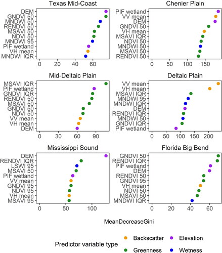
We include example output maps for the Grand Bay estuary in Mississippi for illustrative purposes (Figure 4). The relative importance represented as the mean decrease in Gini for each regional model (Figure 5) points to the elevation-based predictor variables, elevation relative to mean higher high water and/or the probability of an area being an irregularly flooded wetland, as being the most important variables. Specifically, these predictors were among the top-five predictors for all but one region (Deltaic Plain). Mean radar backscatter for VH (vertical transmit/horizontal receive backscatter) and VV (vertical transmit/vertical receive backscatter) were in the top-five most important variables in the Chenier Plain and Deltaic Plain. In contrast, the standard deviation of the radar backscatter was not included in any model. At least one greenness predictor was within the top-five most important predictors for all regions. Among greenness indices, the green normalised difference vegetation index (GNDVI), red edge normalised difference vegetation index (RENDVI), and modified soil adjusted vegetation index (MSAVI) were the most common with four instances each. Normalised difference vegetation index (NDVI) was not in the top-five most important predictors for any region. Of the greenness statistics, the median values for greenness were the most common followed by the interquartile range. Wetness was in the top-five most important predictors for Texas Mid-Coast, Deltaic Plain, and Mississippi Sound, with modified normalised difference water index (MNDWI) being more common than land surface water index (LSWI).

Figure 4. Example of high marsh and salt pannes/flats map products for the Grand Bay estuary, Mississippi, USA. (a) land cover map modified from the National Oceanic and Atmospheric Administration’s Coastal Change Analysis Program 30-m layer (NOAA 2016). (b) map of high marsh, salt pannes/flats, and other irregularly flooded wetlands. (c) map of irregularly flooded wetlands dominated by J. roemerianus. White areas in panes b and c represent areas outside the coastal wetland mask.

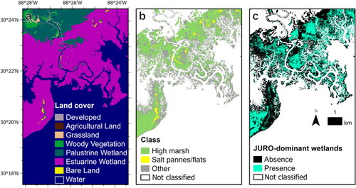
Figure 5. The top 10 predictor variables per region for mapping high marsh and salt pannes/flats along the northern Gulf of Mexico, USA. Predictor importance is proportional to unitless MeanDecreaseGini values. DEM, elevation relative to mean higher high water from the digital elevation model; GNDVI, green normalised difference vegetation index; LSWI, land surface water index; MNDWI, modified normalised difference water index; MSAVI, modified soil-adjusted vegetation index; NDVI, normalised difference vegetation index; PIF, probability irregularly flooded wetland; RENDVI, red edge normalised difference vegetation index; VH, vertical transmit/horizontal receive backscatter; VV, vertical transmit/vertical receive backscatter. Spectral indices that end in 50, 95, IQR, are the median, 95^th percentile, and interquartile range, respectively.

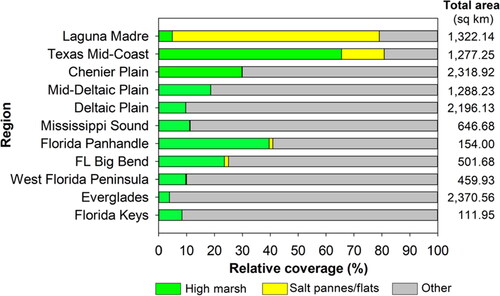
Based on our classification, we estimate a total of 244,261 ha of high marsh, 119,091 ha of salt pannes/flats, and 901,396 ha of wetlands mapped as ‘other’ along the northern Gulf of Mexico coast (Table S2). The relative coverage of high marsh by region (Figure 6) ranged from about 4% to 65%. The highest relative coverage of high marsh occurred in the Texas Mid-Coast, Florida Panhandle, and Chenier Plain with around 65%, 40%, and 30%, respectively. The lowest relative coverage of high marsh was in the Everglades, Laguna Madre, and Florida Keys with about 4%, 5%, and 8%, respectively. The relative coverage of salt pannes/flats by region ranged from approximately 0% to 75%. Everglades, Florida Keys, Mid-Deltaic Plain, and Deltaic Plain, all had little or no coverage of salt pannes/flats. By far, the highest relative coverage of salt pannes/flats was found in Laguna Madre (74%) followed by Texas Mid-Coast with (15%). All maps produced in this study are available via Enwright et al. (2023a).

Figure 6. Relative coverage of high marsh, salt pannes/flats, other irregularly flooded wetlands by region along the northern Gulf of Mexico, USA. Other wetlands had a probability of being irregularly flooded wetland of ≥10% (Enwright et al. 2023b) and were not mapped as high marsh or salt panne/flat. The ‘total area’ column indicates the total area mapped as one of these three classes in square kilometers (sq km). We used sq km instead of ha here due to showing coverage at the region level. See Figure 1 for regional boundaries.

For our 1,641 points, the overall accuracy was 80.99%. The producer’s accuracy was 74.84% and 81.31% for high marsh and salt pannes/flats, respectively. The user’s accuracy was 69.56% and 76.99% for high marsh and salt pannes/flats, respectively (See Table S3 for details).

3.2. Mapping irregularly flooded wetlands dominated by Juncus roemerianus

Regarding importance for mapping irregularly flooded wetlands dominated by J. roemerianus, LSWI variability (IQR) was the most important predictor followed by the median MSAVI, VV and VH mean backscatter, and the median GNDVI (Figure S2). Based on our classification model, there was about 11,885 ha of irregularly flooded wetlands dominated by J. roemerianus from the Mississippi Sound to the Florida Big Bend. The relative coverage of irregularly flooded wetlands dominated by J. roemerianus was about 5%, 16%, and 12% for the Mississippi Sound, Florida Big Bend, and Florida Panhandle, respectively. The areal coverage of irregularly flooded wetlands that were dominated J. roemerianus by region and watershed are included in Table S4.

The overall accuracy of the map of irregularly flooded wetlands dominated by J. roemerianus was 80.00% (n = 155 points). The producer’s accuracy was 63.16% and 89.80% for irregularly flooded wetlands where J. roemerianus is the dominant species and irregularly flooded wetlands not dominated by J. roemerianus, respectively. The user’s accuracy was 78.26% and 80.73% for irregularly flooded wetlands where J. roemerianus is the dominant species and irregularly flooded wetlands not dominated by J. roemerianus, respectively (See Table S5 for details).

4. Discussion

The objective of this study was to develop the first regional map of high marsh and salt panne/flat wetland subsystems across the northern Gulf of Mexico coast. Mapping these subsystems (Figure 4) expands upon the thematic detail for wetlands not explicitly delineated in widely available national mapping products like NOAA’s C-CAP product and the National Wetlands Inventory.

4.1. Comparison with past efforts

Due to their importance for providing fish and wildlife habitat high marsh and salt pannes/flats have been a target for recent mapping efforts nationwide, including: (1) northeastern United States (Correll et al. 2018); (2) southeastern United States (Allen 2017; 2019); (3) Grand Bay estuary, Mississippi (Pitchford 2019); and (4) Texas (Elliott et al. 2014). Earlier mapping efforts utilized high-resolution imagery aerial imagery (Correll et al. 2018; Pitchford 2019); whereas this study, Elliott et al. (2014) and Allen (2017, 2019) used satellite imagery and high-resolution imagery as ancillary data for sample development. Model development in this study was conducted at the regional level similar to Elliott et al. (2014) and Correll et al. (2018). Regional changes in predictor variable composition and order highlighted the benefits of this approach for mapping wetland subsystems along the northern Gulf of Mexico, which features highly variable wetland characteristics (Osland et al. 2014; Gabler et al. 2017).

Elevation has a positive relationship with plant species richness in coastal wetlands (Gough et al. 1994), including the high marsh zone (Brewer et al. 1997). Elevation and tidal information were used by Allen (2017) and Allen (2019) to focus the mapping effort on coastal wetlands, whereas Correll et al. (2018) used elevation data and tidal data to develop elevation thresholds maps. To account for the elevation error in coastal wetlands, which has been well-documented in numerous studies (Enwright et al. 2023b and references therein), our effort utilized elevation data and elevation-based probabilistic maps highlighting the probability of an area being an irregularly flooded wetland. This predictor variable was developed using NOAA’s high tide flooding information as the upper bound of the irregularly flooded wetland zone. Additionally, maps produced here utilized SAR backscatter, which has not been widely used, except by Allen (2017). Incorporating SAR backscatter was important in developing maps for southeastern Louisiana and mapping irregularly flooded wetlands that are dominated by J. roemerianus (Figure S2). We hypothesize this is due to the ability to detect surface roughness, substrate moisture, and vegetation structure in coastal wetlands (Kasischke and Bourgeau-Chavez 1997). Another new element provided here was information on subsystems dominated by J. roemerianus. This information can be used to isolate high marsh areas that are dominated by Spartina patens, Spartina spartinae, and Spartina bakeri, which can be important in areas with extensive J. roemerianus, such as the Grand Bay estuary in Mississippi (Archer et al. 2022). Future mapping efforts could explore expanding a single map with increased thematic resolution that includes high marsh with dominant species (e.g. J. roemerianus-dominated wetlands) and adding SHARP classes (e.g. terrestrial border, low marsh).

Generally, our results confirm findings by Artigas and Yang (2005) that low marsh and high marsh are separable using the red edge and near infrared bands. Specifically, RENDVI was in the top-five most important predictors for four of six regions modelled and at least one of the greenness indices was in the top-five most important predictors for all regions.

Due to the extensive study area, lack of ground reference data across the entire study area, and the complex regional variation of coastal wetlands across the northern Gulf of Mexico (Gabler et al. 2017), our effort focused strictly on mapping high marsh and salt pannes/flats, whereas the other previous efforts mapped a suite of wetland classes. While the map produced in this study spans the entire northern Gulf of Mexico region, areas where multiple maps products exist (e.g. Texas; Grand Bay estuary, Mississippi; and Mobile Bay to Tampa Bay) provide an opportunity for taking an ensemble approach to identifying potential areas that contain high marsh and salt pannes/flats. For example, areas mapped as high marsh in any map could be helpful for users to flag for future investigation.

4.2. Implications

Maps depicting high marsh and salt pannes/flats can serve as a baseline of contemporary wetland coverage and regional variation. It is important to develop efficient and repeatable methods, such as those used here, for developing maps of coastal wetland types over time because coastal wetlands are predicted to undergo widespread transformation due to climate change. Coastal inundation is estimated to increase over the next several decades with accelerated sea-level rise (Sweet et al. 2022). Increased inundation is predicted to lead to the upslope migration of these irregularly flooded wetlands (Osland et al. 2022; Pitchford et al. 2022) or lead to localized loss in areas that cannot keep pace with sea-level change (Saintilan et al. 2022). Mapping these ecosystems at regular intervals can help highlight changes to these important environments. In addition to baseline information, high marsh and salt pannes/flats maps can have numerous applications including: (1) developing new wetland research sites or monitoring (MacKenzie and Dionne 2008); (2) identifying new sites for marsh bird monitoring (Tolliver et al. 2019; Woodrey et al. 2019); (3) highlighting areas for detailed assessments of high marsh, such as the exploration of biomass (Byrd et al. 2018) or microtopography (Stribling et al. 2007); and (4) increasing our understanding and ability to model the distribution of high marsh-dependent species (Tolliver et al. 2019; Stevens et al. 2022).

4.3. Future efforts

The ability to map coastal wetlands has improved due to numerous factors that include: (1) enhanced accessibility to and processing of multitemporal data via cloud computing resources (Wang et al. 2020); (2) increased availability of high-quality elevation data (Enwright et al. 2023b); (3) improved extent and accessibility of radar-based satellite imagery, such as C-band Sentinel-1, and, in the near future, expanded L-band SAR (NASA 2023a); (4) expansion of high-resolution commercial satellite data; (5) data fusion techniques using machine learning algorithms (Worthington et al. 2023); and (6) advancement of deep learning algorithms (Gray et al. 2021). Similar to the increased availability of SAR data, the increased spectral resolution with moderate-resolution satellite imagery planned with Landsat Next should enhance the delineation of marsh types (NASA 2023b). Collectively, these are all avenues for future research to enhance future wetland maps.

In addition to exploring methodology advancements, future efforts can update and enhance the high marsh and salt pannes/flats map produced in this study by filling temporal gaps of elevation data and using new data and data processing techniques. As discussed in Enwright et al. (2023b), since the development of these maps, new lidar data are available in many parts of Florida and data acquisition is planned in parts of coastal Louisiana. Additionally, future efforts could explore enhancing the elevation-based irregularly flooded wetland probability information by using biomass information to add nuance to elevation error assumptions (Enwright et al. 2023b), which could increase the accuracy of the probability outputs in salt pannes/flats. Diagnostic characteristics for high marsh have been developed at the coast-wide level for the Gulf and Atlantic coasts, but regional variability exists in terms of plant species composition (Table S1). Other future enhancements to this specific study could include: (1) collecting data needed to develop models for regions not fitted in this effort; (2) more robust validation, including validating regional boundaries; (3) exploring microtopography in high marsh systems; and (4) the integration of vegetation height above ground metrics from lidar point clouds.

5. Conclusion

We built on past efforts to develop the first regional map of high marsh and salt panne/flat wetland systems across the northern Gulf of Mexico. We accounted for regional variability in wetlands by developing models for regions with available training data. The importance of predictor variables varied by region. In general, elevation, irregularly flooded wetland probability, mean SAR backscatter and spectral indices related to greenness and wetness tended to be the most important for mapping high marsh and salt pannes/flats. The overall accuracy of the high marsh and salt pannes/flats map was just over 80%. The highest relative coverage of high marsh was found in the Texas Mid-Coast, Florida Panhandle, and Chenier Plain, whereas the lowest relative coverage of high marsh was in the Everglades, Laguna Madre, and Florida Keys. By far the highest relative coverage of salt pannes/flats was found in Laguna Madre (74%) followed by Texas Mid-Coast with (15%). Everglades, Florida Keys, Mid-Deltaic Plain, Deltaic Plain, all had no or very little coverage of salt pannes/flat. We created an ancillary map that highlighted J. roemerianus-dominated irregularly flooded wetlands from the Mississippi Sound to the Florida Big Bend. The map had an overall accuracy of 80%. Wetness variability was the most important predictor for this map followed by radar backscatter and greenness indices. Our map and framework advance the collective understanding of estuarine marsh zonation and provide a baseline for assessing future transformations predicted from climate change. The map and framework presented in this study can be updated for this region and adapted to other areas. Future research efforts could explore how these maps can be enhanced using: (1) updates with new lidar data and field data; (2) more robust map validation, including assessing if regional boundaries are appropriate; (3) anticipated satellite sensors and data availability, such as NISAR and the increased spatial and spectral resolution satellite data (e.g. Landsat Next); (4) additional lidar-derivatives, such as height above ground estimates; (5) data fusion; (6) deep learning techniques; and (7) high marsh characteristics, such as microtopography.

Author contributions

NME and KOE designed the research. MSW, AMVF, JAM, and AJN provided review and feedback of study methods. WCC, NME, and HRT performed the data analysis. MSW, JAM, HL, JC, PJK, AJN, and JLP all provided reference data for this study. NME drafted the manuscript, and all authors contributed to the manuscript editing and revision.

Acknowledgments

This paper is a result of research funded by the National Oceanic and Atmospheric Administration’s RESTORE Science Program under award NA19NOS4510195 to Mississippi State University and the U.S. Geological Survey. We thank many individuals for comments on mapping methodology and draft products, including Jacob Berkowitz, Kevin Buffington, Chris Butler, Jeremy Conrad, Warren Conway, Mark Danaher, Rodridgo Diaz, Laura Feher, Christopher Gabler, Elizabeth Godsey, Clay Green, Amanda Haverland, Rebecca Howard, Brita Jessen, Erik Johnson, Kevin Kalasz, Joseph Lancaster, Jonathon Lueck, Jonathan Moczygemba, Michael Osland, Maulik Patel, Sarai Piazza, Colt Sanspree, Amy Schwarzer, Fred Sklar, Eric Soehren, Camille Stagg, Karen Thorne, James Tolliver, William Vermillion, Jenneke Visser, Barry Wilson, Jennifer Wilson, Bernard Wood, Woody Woodrow. Mark S. Woodrey’s participation and contribution is, in part, supported by the National Institute of Food and Agriculture, U.S. Department of Agriculture, Hatch project under accession number 7002261. As such, this publication is considered a contribution of the Mississippi Agricultural and Forestry Experiment Station. J.A. Nyman’s participation and contribution are based upon work that was supported by the National Institute of Food and Agriculture, U.S. Department of Agriculture, McIntire Stennis project under LAB94471. Any opinions, findings, conclusions, or recommendations expressed in this publication are those of the authors and do not necessarily reflect the view of the U.S. Department of Agriculture. Any use of trade, firm, or product names is for descriptive purposes only and does not imply endorsement by the U.S. Government.

Disclosure statement

The authors declare that they have no known competing financial interests or personal relationships that could have appeared to influence the work reported in this paper.

Data availability statement

Data are available as a U.S. Geological Survey data release (Enwright et al. 2023a).

References

- Allen TR. 2017. Marsh classification raster dataset for South Atlantic Landscape Conservation Cooperative [dataset], U.S. Geological Survey. [accessed 2022 May 12]. https://www.sciencebase.gov/catalog/file/get/58f7e41ae4b0b7ea5451fb65?name=MarshDataDownload.zip
- Allen TR. 2019. Marsh habitat mapping and classification synthesis for the Florida peninsula. Norfolk, Virginia: Old Dominion University. https://acjv.org/documents/Report_Florida_Marsh_Habitat_Mapping_2019.pdf.
- Archer MJ, Pitchford JL, Biber P, Underwood W. 2022. Assessing vegetation, nutrient content and soil dynamics along a coastal elevation gradient in a Mississippi Estuary. Estuaries Coasts. 45(5):1217–1229. doi:10.1007/s12237-021-01012-2.
- Artigas FJ, Yang JS. 2005. Hyperspectral remote sensing of marsh species and plant vigour gradient in the New Jersey Meadowlands. Int J Remote Sens. 26(23):5209–5220. doi:10.1080/01431160500218952.
- Barbier EB. 2011. Wetlands as natural assets. Hydrol Sci J. 56(8):1360–1373. doi:10.1080/02626667.2011.629787.
- Barnes E, Clarke TR, Richards SE, Colaizzi PD, Haberland J, Kostrzewski WP, Choi C, Riley E, Thompson T, et al. 2000. Coincident Detection of Crop Water Stress, Nitrogen Status and Canopy Density Using Ground-based Multispectral Data. In: Robert PC, Rust RH, Larson WE, editors. Proceedings of the fifth international conference on precision agriculture. Madison, WI: American Society of Agronomy. p. 1–15.
- Bergstrom JC, Stoll JR, Titre JP, Wright VL. 1990. Economic value of wetlands-based recreation. Ecol Econ. 2(2):129–147. doi:10.1016/0921-8009(90)90004-E.
- Berkowitz JF, Altman S, Reine KJ, Wilbur D, Kjelland ME, Gerald TK, Kim S-C, Piercy CD, Swannack TM, Slack TM, et al. 2020. Evaluation of the potential impacts of the proposed Mobile Harbor navigation channel expansion on the aquatic resources of Mobile Bay, Alabama. ERDC TR-20-4. Vicksburg, MS: engineering Research and Development Center.
- Boesch DF, Turner RE. 1984. Dependence of fishery species on salt marshes: the role of food and refuge. Estuaries. 7(4):460–468. doi:10.2307/1351627.
- Butler CJ, Olsen TW, Kephart B, Wilson JK, Haverland AA. 2022. Interannual Winter Site Fidelity for Yellow and Black Rails. Diversity. 14(5):357. doi:10.3390/d14050357.
- Brewer JS, Levine JM, Bertness MD. 1997. Effects of biomass removal and elevation on species richness in a New England Salt Marsh. Oikos. 80(2):333–341. doi:10.2307/3546601.
- Byrd KB, Ballanti L, Thomas N, Nguyen D, Holmquist JR, Simard M, Windham-Myers L. 2018. A remote sensing-based model of tidal marsh aboveground carbon stocks for the conterminous United States. ISPRS J Photogramm Remote Sens. 139:255–271. doi:10.1016/j.isprsjprs.2018.03.019.
- Cahoon DR. 2006. A review of major storm impacts on coastal wetland elevations. Estuaries Coasts. 29(6):889–898. doi:10.1007/BF02798648.
- Chandrasekar K, Sesha Sai MVR, Roy PS, Dwevedi RS. 2010. Land Surface Water Index (LSWI) response to rainfall and NDVI using the MODIS Vegetation Index product. Int J Remote Sens. 31(15):3987–4005. doi:10.1080/01431160802575653.
- Copernicus Sentinel data 2019–2020. 2021. Retrieved from Google Earth Engine. 7 July processed by the European Space Agency (ESA).
- Copernicus Sentinel data 2020. 2021. Retrieved from Google Earth Engine. 7 July processed by the European Space Agency (ESA).
- CPRA. 2021. Coastwide reference monitoring system. Coastal Information Management System (CIMS) database. Baton Rouge, LA: Coastal Protection and Restoration Authority. https://cims.coastal.la.gov
- Correll MD, Hantson W, Hodgman TP, Cline BB, Elphick CS, Shriver WG, Tymkiw EL, Olsen BJ. 2018. Fine-scale mapping of coastal plant communities in the Northeastern USA. Wetlands. 39(1):17–28. doi:10.1007/s13157-018-1028-3.
- Dale LL, Chivoiu B, Osland MJ, Enwright NM, Thorne KM, Guntenspergen GR, Grace JB. 2022. Estuarine drainage area boundaries for the conterminous United States [dataset]. U.S. Geological Survey. doi:10.5066/P9LPN3YY.
- Elliott LF, Treuer-Kuehn A, Blodgett CF, True CD, German D, Diamond DD. 2014. Ecological Systems of Texas: 391 Mapped Types. Phase 1 – 6, 10-meter resolution Geodatabase, Interpretive Guides, and Technical Type Descriptions [dataset]. Texas Parks & Wildlife Department and Texas Water Development Board. https://tpwd.texas.gov/landwater/land/programs/landscape-ecology/ems
- Ennen JR, Hoffacker ML, Selman W, Murray C, Godwin J, Brown RA, Agha M. 2019. The effect of environmental conditions on body size and shape of a freshwater vertebrate. Copeia. 107(3):550–559. doi:10.2307/26954750.
- Enwright NM, Borchert SM, Day RH, Feher LC, Osland MJ, Wang L, Wang H. 2017. Barrier Island habitat map and vegetation survey—Dauphin Island, Alabama, 2015. Open-File Report 2017–1083. Reston, VA: U.S. Geological Survey. doi:10.3133/ofr20171083.
- Enwright NM, Cheney WC, Evans KO, Thurman HR, Woodrey MS, Fournier AMV, Bauer A, Cox J, Goehring S, Hill H, et al. 2023a. Mapping irregularly flooded wetlands, high marsh, and salt pannes/flats along the northern Gulf of Mexico coast (ver. 2.0, June 2023) [dataset]. U.S. Geological Survey. doi:10.5066/P9MLO26U.
- Enwright NM, Cheney WC, Evans KO, Thurman HR, Woodrey MS, Fournier AMV, Gesch DB, Pitchford JL, Stoker JM, Medeiros SC. 2023b. Elevation-based probabilistic mapping of irregularly flooded wetlands along the northern Gulf of Mexico coast. Remote Sens Environ. 287:113451. doi:10.1016/j.rse.2023.113451.
- Enwright NM, Hartley SB, Couvillion BR, Brasher MG, Visser JM, Mitchell MK, Ballard BM, Parr MW, Wilson BC. 2015. Delineation of marsh types from Corpus Christi Bay, Texas, to Perdido Bay, Alabama, in 2010. Reston, VA: U.S. Geological Survey. doi:10.3133/sim3336.
- Enwright NM, Kranenburg CJ, Patton BA, Dalyander PS, Brown JA, Piazza SC, Cheney WC. 2021. Developing bare-earth digital elevation models from structure-from-motion data on barrier islands. ISPRS J Photogramm Remote Sens. 180:269–282. doi:10.1016/j.isprsjprs.2021.08.014.
- FDEP. 2017. Statewide Land Use Land Cover [dataset]. Tallahassee, FL: Florida Department of Environmental Protection. https://publicfiles.dep.state.fl.us/otis/gis/data/STATEWIDE_LANDUSE.zip.
- Gabler CA, Osland MJ, Grace JB, Stagg CL, Day RH, Hartley SB, Enwright NM, From AS, McCoy ML, McLeod JL. 2017. Macroclimatic change expected to transform coastal wetland ecosystems this century. Nature Clim Change. 7(2):142–147. doi:10.1038/nclimate3203.
- Gitelson AA, Kaufman YJ, Merzlyak MN. 1996. Use of a green channel in remote sensing of global vegetation from EOS-MODIS. Remote Sens Environ. 58(3):289–298. doi:10.1016/S0034-4257(96)00072-7.
- Gough L, Grace JB, Taylor KL. 1994. The Relationship between Species Richness and Community Biomass: the Importance of Environmental Variables. Oikos. 70(2):271–279. doi:10.2307/3545638.
- Gray PC, Chamorro DF, Ridge JT, Kerner HR, Ury EA, Johnston DW. 2021. Temporally Generalizable Land Cover Classification: a Recurrent Convolutional Neural Network Unveils Major Coastal Change through Time. Remote Sensing. 13(19):3953. doi:10.3390/rs13193953.
- Greenberg R, Maldonado JE, Droege S, McDonald MV. 2006. Tidal Marshes: a Global Perspective on the Evolution and Conservation of Their Terrestrial Vertebrates. BioScience. 56(8):675–685. doi:10.1641/0006-3568(2006)56[675:TMAGPO]2.0.CO;2.
- Haverland AA. 2019. Determining the status and distribution of the eastern Black Rail (Laterallus jamaicensis). in coastal Texas [dissertation]. San Marcos, TX: Texas State University-San Marcos.
- Haverland AA, Green MC, Weckerly F, Wilson JK. 2021. Eastern Black Rail (Laterallus jamaicensis jamaicensis) Home Range and Habitat Use in Late Winter and Early Breeding Season in Coastal Texas, USA. Waterbirds. 44(2):222–233. doi:10.1675/063.044.0209.
- Kasischke ES, Bourgeau-Chavez LL. 1997. Monitoring South Florida Wetlands Using ERS-1 SAR Imagery. Photogram Eng Remote Sens. 63(3):281–291.
- Kirwan ML, Guntenspergen GR. 2010. Influence of tidal range on the stability of coastal marshland. J Geophys Res. 115(F2):F02009. doi:10.1029/2009JF001400.
- Krainyk A, Ballard BM, Brasher MG, Wilson BC, Parr MW, Edwards CK. 2019. Decision support tool: mottled duck habitat management and conservation in the Western Gulf Coast. J Environ Manage. 230:43–52. doi:10.1016/j.jenvman.2018.09.054.
- Liaw A, Wiener M. 2002. Classification and Regression by randomForest. R News. 2(3):18–22.
- MacKenzie RA, Dionne M. 2008. Habitat heterogeneity: importance of salt marsh pools and high marsh surfaces to fish production in two Gulf of Maine salt marshes. Mar Ecol Prog Ser. 368:217–230. doi:10.3354/meps07560.
- Mitsch WJ, Gosselink JG. 2007. Wetlands. Hobokes, New Jersey: john Wiley & Sons.
- Mitsch WJ, Wang N. 2000. Large-scale coastal wetland restoration on the Laurentian Great Lakes: determining the potential for water quality improvement. Ecol Eng. 15(3-4):267–282. doi:10.1016/S0925-8574(00)00081-1.
- Möller I, Kudella M, Rupprecht F, Spencer T, Paul M, van Wesenbeeck BK, Wolters G, Jensen K, Bouma TJ, Miranda-Lange M, et al. 2014. Wave attenuation over coastal salt marshes under storm surge conditions. Nature Geosci. 7(10):727–731. doi:10.1038/ngeo2251.
- Moon JA, Feher LC, Lane TC, Vervaeke WC, Osland MJ, Head DM, Chivoiu BC, Stewart DR, Johnson DJ, Grace JB, et al. 2022. Surface elevation change dynamics in coastal marshes along the northwestern Gulf of Mexico: anticipating effects of rising sea-level and intensifying hurricanes. Wetlands. 42(5):49. doi:10.1007/s13157-022-01565-3.
- Moon JA, Lehnen SE, Metzger KL, Squires MA, Brasher MG, Wilson BC, Conway WC, Haukos DA, Davis BE, Rohwer FC, et al. 2021. Projected impact of sea-level rise and urbanization on mottled duck (Anas fulvigula) habitat along the Gulf Coast of Louisiana and Texas through 2100. Ecol Indic. 132:108276. doi:10.1016/j.ecolind.2021.108276.
- Morris JT, Edwards J, Crooks S, Reyes E. 2012. Assessment of Carbon Sequestration Potential in Coastal Wetlands. In: Lal R, Lorenz K, Hüttl R, Schneider B, von Braun J, editors. Recarbonization of the Biosphere. Dordrecht: Springer. p. 517–531.
- Morris JT, Sundareshwar PV, Nietch CT, Kjerfve B, Cahoon DR. 2002. Responses of coastal wetlands to rising sea level. Ecology. 83(10):2869–2877. doi:10.1890/0012-9658(2002)083[2869:ROCWTR]2.0.CO;2.
- Morris KM, Woodrey MS, Hereford SG, Soehren EC, Conkling TJ, Rush SA. 2017. Yellow Rail (Coturnicops noveboracensis) occupancy in the context of fire in Mississippi and Alabama, USA. Waterbirds. 40(2):95–104. doi:10.1675/063.040.0202.
- NASA. 2023a. NISAR-ISO SAR mission. Pasadena, CA: NASA Jet Propulsion Laboratory. [accessed 2023 June 18]. https://nisar.jpl.nasa.gov/.
- NASA. 2023b. Landsat Next. Pasadena, CA: NASA Jet Propulsion Laboratory. https://landsat.gsfc.nasa.gov/satellites/landsat-next/.
- NOAA. 2016. NOAA's Coastal Change Analysis Program (C-CAP) 2016 Regional Land Cover Change Data – Coastal United States [dataset]. Office for coastal management. https://coast.noaa.gov/digitalcoast/data/ccapregional.html
- NOAA. 2019a. Tide Tables 2020: east Coast of North and South America. Silver Spring, MD: National Ocean Service. https://tidesandcurrents.noaa.gov/tidetables/2020/ectt_2020_full_book.pdf.
- NOAA. 2019b. 2015–2017 C-CAP Derived 10 meter Land Cover – BETA [dataset]. NOAA Office for Coastal Management. https://coast.noaa.gov/digitalcoast/data/ccapderived.html
- Novoa V, Rojas O, Ahumada-Rudolph R, Sáez K, Fierro P, Rojas C. 2020. Coastal wetlands: ecosystems affected by urbanization? Water. 12(3):698. doi:10.3390/w12030698.
- Osland MJ, Chivoiu B, Enwright NM, Thorne KM, Guntenspergen GR, Grace JB, Dale LL, Brooks W, Herold N, Day JW, et al. 2022. Migration and transformation of coastal wetlands in response to rising seas. Sci Adv. 8(26):eabo5174. doi:10.1126/sciadv.abo5174.
- Osland MJ, Enwright N, Stagg CL. 2014. Freshwater availability and coastal wetland foundation species: ecological transitions along a rainfall gradient. Ecology. 95(10):2789–2802. doi:10.1890/13-1269.1.
- Osland MJ, Stevens PW, Lamont MM, Brusca RC, Hart KM, Waddle JH, Langtimm CA, Williams CM, Keim BD, Terando AJ, et al. 2021. Tropicalization of temperate ecosystems in North America: The northward range expansion of tropical organisms in response to warming winter temperatures. Glob Chang Biol. 27(13):3009–3034. doi:10.1111/gcb.15563.
- Pitchford JL. 2019. GND_HRLC_AA_05032015_edited [dataset]. National Estuarine Research Reserve System Central Data Management Office. https://cdmo.baruch.sc.edu/get/gis_index.cfm.
- Pitchford JL, Cressman K, Cherry JA, Russell BT, McIlwain J, Archer MJ, Underwood WV. 2022. Trends in surface elevation and accretion in a retrograding delta in coastal Mississippi, USA from 2012–2016. Wetlands Ecol Manage. 30(3):461–475. doi:10.1007/s11273-022-09871-7.
- Probst P, Wright MN, Boulesteix AL. 2019. Hyperparameters and tuning strategies for random forest: wiley Interdisciplinary Reviews. Data Mining Knowledge Disc. 9:e1301. doi:10.1002/widm.1301.
- Qi J, Chehbouni A, Huete AR, Kerr YH, Sorooshian S. 1994. A modified soil adjusted vegetation index. Remote Sens Environ. 48(2):119–126. doi:10.1016/0034-4257(94)90134-1.
- R Core Team. 2018. R: A language and environment for statistical computing. Vienna: R Foundation for Statistical Computing.
- Rasser MK, Fowler NL, Dunton KH. 2013. Elevation and plant community distribution in a microtidal salt marsh of the Gulf of Mexico. Wetlands. 33(4):575–583. doi:10.1007/s13157-013-0398-9.
- Reed DC, Schmitt RJ, Burd AB, Burkepile DE, Kominoski JS, McGlathery KJ, Miller RJ, Morris JT, Zinnert JC. 2022. Responses of Coastal Ecosystems to Climate Change: insights from Long-Term Ecological Research. BioScience. 72(9):871–888. doi:10.1093/biosci/biac006.
- Rogers AS, Kearney MS. 2004. Reducing signature variability in unmixing coastal marsh Thematic Mapper scenes using spectral indices. Int J Remote Sens. 25(12):2317–2335. doi:10.1080/01431160310001618103.
- Rouse JW, Haas RH, Schell JA, Deering DW. 1974. Monitoring vegetation systems in the Great Plains with ERTS. In: Freden SC, Mercanti EP, Becker M, editors. Third Earth Resources Technology Satellite–1 Symposium, Volume I: Technical Presentations, NASA SP-351. Washington, DC: NASA. p. 309–317.
- Saintilan N, Kovalenko KE, Guntenspergen G, Rogers K, Lynch JC, Cahoon DR, Lovelock CE, Friess DA, Ashe E, Krauss KW, et al. 2022. Constraints on the adjustment of tidal marshes to accelerating sea level rise. Science. 377(6605):523–527. doi:10.1126/science.abo7872.
- Schneider SA, Broadley HJ, Andersen JC, Elkinton JS, Hwang S-Y, Liu C, Noriyuki S, Park J-S, Dao HT, Lewis ML, et al. 2022. An invasive population of Roseau Cane Scale in the Mississippi River Delta, USA originated from northeastern China. Biol Invasions. 24(9):2735–2755. doi:10.1007/s10530-022-02809-3.
- Sievers M, Brown CJ, Tulloch VJD, Pearson RM, Haig JA, Turschwell MP, Connolly RM. 2019. The role of vegetated coastal wetlands for marine megafauna conservation. Trends Ecol Evol. 34(9):807–817. doi:10.1016/j.tree.2019.04.F004.
- Stagg CL, Osland MJ, Moon JA, Hall CT, Feher LC, Jones WR, Couvillion BR, Hartley SB, Vervaeke WC. 2020. Quantifying hydrologic controls on local- and landscape-scale indicators of coastal wetland loss. Ann Bot. 125(2):365–376. doi:10.1093/aob/mcz144.
- Stevens BS, Conway CJ, Luke K, Weldon A, Hand CE, Schwarzer A, Smith F, Watson C, Watt BD. 2022. Large-scale distribution models for optimal prediction of Eastern black rail habitat within tidal ecosystems. Global Ecol Conserv. 38:e02222. doi:10.1016/j.gecco.2022.e02222.
- Stribling JM, Cornwell JC, Glahn OA. 2007. Microtopography in tidal marshes: ecosystem engineering by vegetation? Estuaries Coasts. 30(6):1007–1015. doi:10.1007/BF02841391.
- Sweet WV, Hamlington BD, Kopp RE, Weaver CP, Barnard PL, Bekaert D, Brooks W, Craghan M, Dusek G, Frederikse T. 2022. Global and Regional Sea Level Rise Scenarios for the United States: updated Mean Projections and Extreme Water Level Probabilities Along U.S. Coastlines. Technical Report NOS 01. Silver Spring, MD: National Oceanic and Atmospheric Administration, National Ocean Service, NOAA.
- Thompson PR, Widlansky MJ, Hamlington BD, Merrifield MA, Marra JJ, Mitchum GT, Sweet W. 2021. Rapid increases and extreme months in projections of United States high-tide flooding. Nat Clim Chang. 11(7):584–590. doi:10.1038/s41558-021-01077-8.
- Thorne K, Jones S, Freeman C, Buffington K, Janousek C, Guntenspergen G. 2022. Atmospheric River Storm Flooding Influences Tidal Marsh Elevation Building Processes. JGR Biogeosciences. 127(3):e2021JG006592. doi:10.1029/2021JG006592.
- Tolliver JDM, Moore AA, Green MC, Weckerly FW. 2019. Coastal Texas black rail population states and survey effort. J Wildl Manag. 83(2):312–324. doi:10.1002/jwmg.21589.
- U.S. Fish and Wildlife Service. 2022. USFWS National Wetlands Inventory [dataset]. U.S. Fish and Wildlife Service. [Accessed 8 July 2022]. https://www.fws.gov/program/national-wetlands-inventory.
- USGS. 2020. USGS national map 3DEP downloadable data collection [dataset]. USGS. https://nationalmap.gov/3DEP/
- USNVC. 2022. United States national vegetation classification database 2.0.4. Washington DC: federal Geographic Data Committee, Vegetation Subcommittee. https://usnvc.org/
- Wang H, Dai Z, Trettin CC, Krauss KK, Noe GB, Burton AJ, Stagg CL, Ward EJ. 2022. Modeling impacts of drought-induced salinity intrusion on carbon dynamics in tidal freshwater forested wetlands. Ecol Appl. 32(8):e2700. doi:10.1002/eap.2700.
- Wang X, Xiao X, Zou Z, Hou L, Qin Y, Dong J, Doughty RB, Chen B, Zhang X, Chen Y, et al. 2020. Mapping coastal wetlands of China using time series Landsat images in 2018 and Google Earth Engine. ISPRS J Photogramm Remote Sens. 163:312–326. doi:10.1016/j.isprsjprs.2020.03.014.
- Wieland RG. 2007. Habitat types and associated ecological communities of the Grand Bay National Estuarine Research Reserve. In: Peterson, MS, Waggy, GL, Woodrey, MS, editors. Grand bay national estuarine research reserve: an ecological characterization. Moss Point, MS: Grand Bay National Estuarine Research Reserve. p. 103–147.
- Woodrey MS, Fournier AMV, Cooper RJ. 2019. GoMAMN strategic bird monitoring guidelines: marsh Birds. In: Wilson RR, Fournier AMV, Gleason JS, Lyons JE, Woodrey MS, editors, Strategic bird monitoring guidelines for the Northern Gulf of Mexico. Mississippi agricultural and forestry experiment station research bulletin 1228. Starkville, MS: Mississippi State University. p. 71–96.
- Worthington TA, Spalding M, Landis E, Maxwell TL, Navarro A, Smart LS, Murray NJ. 2023. The distribution of global tidal marshes from earth observation data. BioRxiv. doi:10.1101/2023.05.26.542433.
- Xu H. 2006. Modification of normalised difference water index (NDWI) to enhance open water features in remotely sensed imagery. Int J Remote Sens. 27(14):3025–3033. doi:10.1080/01431160600589179.