Are public green spaces distributed fairly? A nationwide analysis based on remote sensing, OpenStreetMap and census data

Abstract

Green space (GS) is a crucial resource in urban areas, but not spatially uniformly distributed. We compare the availability of GS on a national scale using green land cover (GLC) and public green space (PGS). Using spatial census data we analyse GS availability and accessibility for the German population. The average GS availability differs by a factor of three between GLC and PGS. 19.2 % of Germans find less than the WHO defined target for PGS in their neighbourhood. PGS is less equally distributed among the population than GLC, and green space equity varies significantly between rural and urban areas. In areas with multi-family homes, a higher share of the population has access to sufficient PGS than in areas with predominantly single-family homes. We find a negative relation between GLC availability and share of immigrant population, which does not extend to PGS.

Keywords:

• Public green space
• green land cover
• environmental justice
• remote sensing
• OpenStreetMap

1. Introduction

Urban green spaces (UGS) are studied as part of a very active field of geographic environmental justice (EJ) research (Weigand et al. 2019; Zhuang et al. 2022). Many studies analyse the positive effects of local urban green infrastructure on (micro-) climate (Middel et al. 2014), health (e.g. Maas et al. 2006; Villeneuve et al. 2012; Richardson et al. 2013; Honold et al. 2016), well-being and social inclusion (Lee and Maheswaran 2011; Pope et al. 2015). The latter effects gained particular prominence among urban populations around the world as the COVID-19 pandemic increased mental health issues in societies around the world including anxiety, confusion, stress and many more (World Health Organization 2020). It is therefore no surprise that green spaces are important factors for improving quality of life (Sapena et al. 2021; Castelli et al. 2023) and further, green spaces rank among the most important drivers for influencing residential location decisions (Wurm et al. 2019c). That is, the United Nations recognize urban green spaces in goal 11.7 of the Sustainable Development Goals that aims to ‘provide universal access to safe, inclusive and accessible, green and public spaces, in particular for women and children, older persons and persons with disabilities’ (UN General Assembly 2015, p. 22).

Disproportionate access to green spaces has been identified as a critical concern of EJ (e.g. Jennings et al. 2012; Rigolon 2016; Zuniga-Teran and Gerlak 2019; Schüle et al. 2019). That is, generally speaking, some neighbourhoods have access to more or higher quality green spaces than others (e.g. Jünger 2021) making the spatial distribution of UGS an issue of social equity. However, not all green spaces in the urban layout provide similar salutogenic benefits (e.g. Wheeler et al. 2015; Akpinar et al. 2016; Mears et al. 2020). One essential type of UGS with high relevance for public health and social cohesion in cities are publicly accessible green spaces (PGS) (Gómez-Baggethun et al. 2013; Ludwig et al. 2021). Expectedly, they serve as an indispensable resource for people without private gardens (Poortinga et al. 2021) but also provide valuable services to those with access to private green (Lin et al. 2014; Berdejo-Espinola et al. 2021).

Despite the relevance, a lack of suitable, accessible, high-resolution, large-scale data has been identified a central limiting factor for more comprehensive and detailed studies on urban green (Feltynowski et al. 2018). However, freely accessible geodata have the potential to fill data gaps and expand the spatial coverage of EJ studies. They allow capturing differences in the availability of green spaces beyond urban agglomerations and thus allow broadening social equity studies to larger areas or increase their spatial detail. Many studies in the domain of urban green have already used remote sensing imagery to derive land cover and land use information about UGS (Weigand et al. 2019). Therein, higher spatial resolution imagery contributes to a more reliable estimation of greenness especially in local applications (Jimenez et al. 2022). Green Land Cover (GLC) data and vegetation indices are accessible metrics for quantifying the greenness of an area (e.g. Dewulf et al. 2016; Santos et al. 2016; Russette et al. 2021). However, such data often fails to differentiate between different types of green spaces by land use, e.g. between grass covered agricultural meadows and parks and urban gardens. In the vast body of literature there are stark differences in how urban green is mapped and analysed (Kabisch 2019) and studies analysing ‘green space’ frequently fail to define it sufficiently which can lead to incompatibilities or even diverging results between results (Taylor and Hochuli 2017; Wüstemann et al. 2017; Klompmaker et al. 2018).

To solve this, open geodata can be used to derive more detailed and semantically differentiated green space geoinformation. Recent studies have demonstrated the use of data fusion between satellite imagery and volunteered geographic information (VGI) expanding knowledge beyond land cover and derive high detail land use information (Ludwig et al. 2021; Rosier et al. 2022). VGI provide rich semantic attributes of land use that go beyond physical description of land cover (Vargas-Munoz et al. 2021). This can extend the analyses of UGS by differentiating types of green, such as forests or parks from green agricultural areas.

Beyond that, analyses across multiple cities reveal different patterns of greenness between cities (Kabisch et al. 2016; Wüstemann et al. 2017; Zepp et al. 2020; Taubenböck et al. 2021). Yet, many studies focus on individually selected cities, excluding the rural regions around them. In fact, most studies researching the health effects, distribution, and equity of green space focus on localized case studies in urbanized regions (Weigand et al. 2019). Still, for example in Germany, only 50 % to 68.1 % of the population live in urbanized regions depending on the concept urbanization, the data, the spatial units of measurement, the variables, or the thresholds applied (Taubenböck et al. 2022). In light of the known variance in UGS availability, a large scale expansion of green space evaluation to suburbs and rural regions can bring a broader perspective for social equity research.

In this paper, we analyse the distribution of green space availability with high-resolution geographic data on national scale. To do so, we use a combination of different data sets: remote sensing imagery, VGI vector data and spatially explicit socioeconomic and demographic data. We quantify the availability of green space on neighbourhood level for the entire population of Germany via two green space metrics: (1) green land cover (GLC) availability and (2) public green space (PGS) availability. This is to scrutinize the differences in availability depending on the type of green. We quantify the distributive inequality (Enssle and Kabisch 2020) of the resource GLC/PGS using descriptive statistics and multivariate mixed effects regression models for the relationship between GLC/PGS and demographic composition. Our research aims to answer the following research questions:

RQ1: Which share of the German population have sufficient access to green space?

RQ2: How is GS availability distributed in the German population beyond major cities, between rural and urban regions, or neighbourhood housing types?

RQ3: How does neighbourhood population composition relate to green space availability? How does it differ between GLC and PGS?

2. Conceptualizing ‘public green space’

Cities are often touting themselves as ‘the greenest city’. But even on macro scales, the greenness of a city is strongly dependent on the objectivity of the data used to analyse and the definition of the spatial scope and thus can vary widely across metrics (Taubenböck et al. 2021). These variances increase even more on local scales (Wüstemann et al. 2017). Beyond that, not all green is equally relevant from a health perspective (Mears et al. 2020). Roadside greenery might have a positive impact on air quality (Pugh et al. 2012), but it does not serve as a place for physical activity or social gathering. Similarly, a private garden or allotments might serve as a place of refuge from the hectic city for some, but they are generally not available to the public. Hence, when going beyond the question of ‘How green is a city?’, and towards ‘How much publicly accessible green space, parks and gardens are in a city?’ it is important to be able to distinguish between different types of green. Thus, it is necessary to go beyond the physical representation of green patches in the (urban) landscape, i.e. land cover, and add semantic information on the type of green, i.e. land use.

Green space typically refers to vegetated, open and unsealed land and thus differs from built urban landscapes of buildings and roads (Swanwick et al. 2003; Jorgensen and Gobster 2010; Hunter and Luck 2015). Located in the vicinity of urban settlements these green spaces are also referred to as urban green space (UGS, Jim and Chen 2006). In cities this includes parks, gardens, forests, certain sports facilities, but also abandoned areas or industrial patches. Beyond the city borders, natural landscapes, forests, meadows, and the like can be considered to be natural greens. Depending on the type or accessibility, green spaces serve various environmental purposes and provide different services.

In this study, we define public green space (PGS) in accordance with Ludwig et al. (2021) as vegetated or natural areas that generally can be assumed to be freely accessible by the public. This includes forests, wilderness areas, urban parks, playgrounds, and public gardens. In contrast, non-public green spaces differ in that they are privately owned and may be excluded from free public access and use. This is usually the case for private gardens, areas with limited or member-only access like sports facilities or allotments, industrial or commercial areas, agricultural crops, airfields, restricted military areas, or otherwise unusable greened or vegetated land. We focus on the availability, i.e. the amount of PGS in hectares, as this is a robust metric of intra-city inequalities compared to, for example, distance based metrics (Rigolon 2016).

Green space availability can be measured at varying spatial scales. For example, some studies use the average green space in administrative spatial units or zip-code areas with wide variation in size, urbanity, and population (e.g. Akpinar et al. 2016). This, however can lead to bias caused by the modifiable areal unit problem (MAUP, Openshaw 1983), which means the outcome of the analysis might be skewed by the arbitrary layout of the spatial units. We aim at reducing MAUP bias through working with standardized spatial units for the entire study area. In particular, we focus on the availability of green space in the living environment of the people, specifically the neighbourhood at their home address. In the literature on urban green we find several definitions for the neighbourhood (for a comprehensive review see Kabisch 2019). Often these are delineated around the home address with varying distance, e.g. 300 m (Xu et al. 2018a, 2018b; Wolff and Haase 2019; Barber et al. 2021; Long et al. 2022), 400 m (Flacke et al. 2016), 500 m (Wüstemann et al. 2017), 100 m − 3000 m (Klompmaker et al. 2018). We choose the distance Kabisch (2019) identified as the most prevalent in recent studies, a 500 m radius neighbourhood, since the surrounding neighbourhood strongly influences the individual perception of urban structure (Wurm et al. 2019a) and thus affects habits of pedestrian movement (Droin et al. 2023).

3. Data and methods

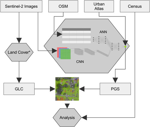
Figure 1 shows the workflow of this study. GLC and PGS availability were derived from different input data to enable a nationwide analysis of green space in Germany.

Figure 1. Workflow of this study. The GLC dataset is derived from a land cover classification (*) developed by Weigand et al. (2020) and PGS is derived from a deep learning data fusion (see sec. 3.1.2). both datasets are used in conjunction with nationwide census data to support the analyses in this study.

3.1. Data and preprocessing

To facilitate a comparison between local-scale GLC and PGS and the analysis of social equity in their availabilities for the entire population of Germany several datasets were used in this study: (1) GLC data was derived from a high-resolution satellite image classification, (2) PGS data was derived using data fusion of satellite imagery and VGI vector data. These datasets allowed to quantify green space availability by means of two different metrics. (3) Spatial population data was used from a national census to allow for population weighted analyses.

3.1.1. Green land cover

The availability of green land cover on neighbourhood level was derived from Sentinel-2-based land cover classification. The national land cover product with a 10 m × m spatial resolution was created as described by Weigand et al. (2020) based on Sentinel-2 imagery. The Land Use and Coverage Area Frame Survey (LUCAS)¹ conducted by Eurostat 2018 served as ground reference. This dataset made use of all Sentinel-2 L1C scenes acquired over Germany between May and September 2018 with less than 60 % cloud cover. Further cloud masking was performed using the Sentinel-2 QA60 band, before a median mosaic was derived from all scenes. Using a diverse set of spectral indices and image features, a random forest classification algorithm was trained to derive the final land cover classification. It contained a total of seven land cover classes (for more detail see Weigand et al. 2020) and achieved an overall accuracy of 90.93 %, thus outperforming comparable continental or global scale land cover classifications (e.g. Pflugmacher et al. 2019; Brown et al. 2022). In the scope of the present study, tree cover and grasslands were considered as green land cover (GLC), specifically the classes low perennial vegetation, high perennial vegetation and high seasonal vegetation. These refer to grassland, lawns and meadows as well as tree cover in parks and forests. This GLC dataset al.lowed for quantifying the availability of general green space. It did not distinguish, however, between different types by, e.g. ownership, accessibility, form, or use.

3.1.2. Public green space

To expand the analysis beyond the mere physical description of urban green via GLC, a spatio-quantitative data on PGS was derived to represent one specific type of green space. Like in previous studies (e.g. Kabisch and Haase 2014; Krekel et al. 2016; Wüstemann et al. 2017; Liao et al. 2021), data from the 2018 European Urban Atlas ² (EUA) was used as a base to quantify PGS availability. PGS was defined as the EUA classes Green urban areas, Forests and Herbaceous vegetation associations. However, the EUA dataset did not cover the entire area of Germany but only 96 spatial functional urban areas encompassing 75 % of the population. To extend the analyses beyond the borders of these areas and hence, to cover the entirety of Germany, PGS availability was extrapolated using data fusion of multiple spatially exhaustive datasets and a machine learning approach. Similar to recent approaches combining satellite image data and vector based geographic data (Rosier et al. 2022; Georganos et al. 2022), satellite imagery and OpenStreetMap (OSM) data were combined to model the target measure: the amount of available PGS in the neighbourhood. The decision to use a model for estimating neighbourhood greenness was influenced by two factors. First, this allowed to conflate differences in the definition of land use between EUA and OSM and thus increase comparability with previous studies that used EUA. Second, opposed to a pure geometric approach which uses the OSM polygons, this approach allowed for incorporating a diverse set of OSM features to quantify public green availability and is thus less prone to errors from falsely tagged or missing polygons of public green spaces in the OSM database. As it has been shown that different classes of urban green feature varying degrees of correctness and completeness (Dorn et al. 2015), estimating PGS availability through a model incorporating satellite imagery and OSM features provided a stable yet scalable solution to apply in the nationwide scope of this study compared to relying on individual polygon features.

The 2018 Sentinel-2 mosaic previously used for the creation of the land cover classification (cf. sec. 3.1.1) was used for the image data in the data fusion. We extracted three Sentinel-2 bands, i.e. the red, green, and blue channels as well as a derived NDVI image. Additionally, the previously derived land cover classification was included as a fifth image layer. All layers had a spatial resolution of 10 m × 10 m.

OpenStreetMap contains geographical features as a collection of vector data in form of points, lines, and polygons. In this study, these were converted to tabular data through spatial aggregation on neighbourhood level. Features relevant for quantifying the absence or presence of public green spaces were identified by means of their attribute data in form of annotated key = value pairs, also referred to as tags. Using these tags, all OSM features relevant for this study were grouped into semantically consistent collections of different tags. This was done to consolidate similar information from related tags. Overall, a total of 71 groups were formed combining similar aspects indicating absence or presence of public green space, access of areas to the public, or other relevant land use features. The full table of OSM groups can be found in the supplemental materials of this study. As one example, the group ‘public leisure’ includes all features tagged with ‘leisure = common’, ‘leisure = dog_park’, ‘leisure = fitness_station’, ‘leisure = nature_reserve’, ‘leisure = park’, ‘leisure = picnic_table’, ‘leisure = playground’, and ‘leisure = slipway’.

For each neighbourhood, features of all geometry types – points, lines and polygons – were aggregated for each group. Points were aggregated by count, lines by cumulative length, and polygons by cumulative area. In total, 94 metrics were derived from the 71 groups as some groups were represented by multiple geometry types.

Subsequently, a deep learning-based data fusion network combining raster format image data and tabular OSM aggregates was established³. The aim of this approach was to utilize the information from both data sources simultaneously, leveraging the combined predictive power of both datasets. Therein, image data served as input for a convolutional neural network (CNN) developed for land cover classification (Qiu et al. 2020; Wurm et al. 2019b). OSM data was fed into an artificial neural network (ANN). Determined by the number of OSM aggregates, the ANN has 94 input nodes. These are followed by hidden layers with 20, 10 and 5 nodes. All nodes are followed by batch normalization and ReLU-activation (Fukushima 1969; Goodfellow et al. 2016, p. 187). Batch normalization (Ioffe and Szegedy 2015) is used to avoid extreme values within the network and is therefore an effective means optimization of the network (Goodfellow et al. 2016, p. 309 ff.). A dropout layer was placed before the final layer. The network architecture can be found in the supplemental materials. Both networks were pre-trained individually on the PGS target first to improve convergence of the network. Subsequently, they combined and trained as a fusion network. The fusion network extends the ANN and CNN by concatenating their last dense layer into a shared fusion layer followed by three dense layers until they reach the final regression layer. During the learning process, we used Huber loss to optimize the model’s regression performance. The target to predict was the available area of PGS in a neighbourhood. During training, we used a batch size of 512 observations, a dropout rate of 0.1, an initial learning rate of 0.0001, with a learning rate reduction on plateaus after 20 epochs and early stopping after 40 epochs. Further, the parameters underwent a warm-up period of three epochs with a learning rate of 1× 10^-15.

The model was trained using 115,220 roughly 1 km² sized tiles (101 $\times$ 101 Sentinel-2 pixels) across Germany, the total number of neighbourhoods fully covered by EUA reference data. To ensure independence between the model training and evaluation data, all neighbourhoods were split into training, validation, and test datasets holding 70 %, 15 %, and 15 % of the data, respectively. The spatially independent test dataset was used to evaluate the PGS model yielding a high coefficient of agreement ($R^2=0.952$) and very low mean absolute error (MAE = 3.2 %).

Ultimately, this model was able to predict the PGS availability in any rectangular neighbourhood enclosing a 500 m wide buffer around a central point, beyond any arbitrary spatial border of the functional urban areas covered by the EUA. Trained and tested on the 115,200 tiles across EUA regions in Germany, this model was used in this study to determine the available neighbourhood PGS for the neighbourhood of every location registered in the nationwide geolocalized gridded census data. In total this amounts to 3.1 million neighbourhoods.

3.1.3. Population data and housing type

For locating the population in Germany, the latest available census information from the 2011 census was used. The German Federal Statistical Office (destatis) provides demographic population data in spatial grids following the INSPIRE standard⁴. In the census grid data, individuals are located to a specific grid cell by means of address location. Every cell is spatially referenced by its centre point for combination with GLC and PGS availability. This official dataset provides a standardized source of population distribution across Germany. All location data from the census 2011 grids underlie perturbation measures to ensure privacy.

In this study, three different datasets were derived from the 2011 census. First, the total population count which was provided in a 100 m $\times$ 100 m (1 ha) INSPIRE conform grid dataset. This dataset enabled the population weighted analysis of the distribution of GLC/PGS and thus to quantify the share of the population affected by different availabilities of GS.

Second, also on the spatial basis of 1 ha grid cells, the 2011 German census data includes spatial assessment of housing types throughout Germany, namely the number of houses by type. In the present study, this information was used to analyse how particular housing types are associated with different green space availability patterns. At the spatial level of 1 ha, the census aggregates the number of buildings in 7 classes. They were aggregated into four types as detailed in Table 1. For the purpose of analysing green space availability, only census grid cells that contain at least five buildings and only have buildings of the same aggregated class were selected.

Table 1. Aggregation scheme for census building type classification.

Aggregated type	N Cells	Census building type
Detached house	716949	Detached single-family home
		Detached two-family home
Semi-detached house	42066	Semi-detached single-family home
		Semi-detached two-family home
Terraced house	34425	Terraced single-family home
		Terraced two-family home
Multi-family home	22214	Multi-family home 3 - 6 flats
		Multi-family home 7 - 12 flats
		Multi-family home 13 flats or more

For each aggregated class, the number of neighbourhoods (N cells) with buildings of exclusively one aggregated building type and at least 5 buildings are summarized.

The third dataset derived from the 2011 Census was aggregate demographic information about neighbourhood population composition. These data are provided at the spatial resolution of 1 km × 1 km (1 km²) grid cells. For analysing the relationship between GS and demographic composition at 1 km × 1 km resolution, GLC and PGS availability was acquired as the average from the values ascribed to all underlying 100 m × 100 m census grid cells. Three demographic composition metrics were used including information about certain broadly defined society groups regularly found in the literature about green space, e.g. the share of children under 18 years (Rehling et al. 2021), elderly, aged 65 and above (Artmann et al. 2019; Kabisch and Haase 2014), and foreigners (Jünger 2021), i.e. persons with no German citizenship.

3.1.4. Rural-urban gradient

Different green space availability were expected between rural and urban regions. Therefore, all neighbourhoods were analysed with respect to the population of the municipality. Classes were created along the thresholds of 5,000, 10,000, 50,000, and 100,000 inhabitants. Each census grid cell was assigned to a municipality based on the intersection between the centre coordinate and the administrative boundaries of Germany.

To understand the relationship between the urban context of a neighbourhood and green space availability even better, data on the rural-urban gradient were used from Taubenböck et al. (2022). This classification between ‘the rural’ and ‘the urban’ is based on a variety of administrative and grid-based classifications of the degree of urbanization. From all variants a probability-based metric is derived to generate a final classification of the urban-rural gradient. Thus, every populated neighbourhood in Germany is assigned to one of five classes from ‘the rural’ to ‘the urban’ based on quantiles of urbanity. This dataset was relevant for the present study because it allowed a finer-grained discrimination between different grades of urbanity on a sub-municipality level. This increased the interpretability as it allowed for the gradual differentiation between the urban centres and the outskirts of cities and towns.

3.2. Methods

3.2.1. Descriptive statistics

First, local-scale availability of GLC and PGS at national level was analysed using descriptive statistics. As a baseline for analysing social equity of green space availability, it was compared which share of the population in Germany has access to sufficient amounts of public green. Based on goals set by the World Health Organization (2017), residents should find at least 1.8 ha to 3.6 ha of PGS within the 500 m neighbourhood used in this study. Here, it was assumed that social equity of public green access in Germany would exist if the entire population lived in neighbourhoods with more than 3.6 ha of PGS available.

In addition to PGS, the GLC availability in all neighbourhoods in Germany was quantified. As GLC is a superset of green spaces, i.e. it includes many more green space types besides PGS, different thresholds were established. Neighbourhoods were split into tertiles by GLC (low, medium, high) based on the population-weighted distribution in Germany. This resulted in thresholds for GLC at 25.4 and 44.2 ha.

To reduce complexity and aid readability, a two-dimensional classification scheme using the GLC and PGS thresholds was adopted. This was done in order to better understand the composition of green spaces at the neighbourhood level through the co-occurrence of GLC and PGS values. The classification scheme was used to calculate the cumulative shares of population for each class of GS availability. This allowed for the identification of disparities among the population and the quantification of the share of population with below-target PGS availability. Therein, the spatial nature of the census grid was used to apply different grouping strategies: entire Germany, by municipality size, fine-grained rural-urban gradient, and dominant housing type.

3.2.2. Distributive equality of green space

The Gini coefficient is a measure of inequality of distribution or concentration. It can be used to quantify the distributive equality of a resource within a population and is applied to assess social equity of spatial green space distribution (e.g. Kabisch and Haase 2014; Xu et al. 2018b). In this study the Gini coefficient was used to assess the distributive equality of both GLC and PGS among the German population. The Gini coefficient G is defined as (1) $$G=\frac{\sum _{i=1}^n\sum _{j=1}^n\left|x_i-x_j\right|}{2n\sum _{j=1}^n{x}_j}$$(1) where x_i is the available green space for an individual i of the population of n people. The Gini coefficient ranges from 0, indicating fully equal distribution of the resource, to 1, indicating the most unequal distribution possible, i.e. the accumulation of the available resource for only one individual, or in this study one census grid cell. Accompanying the Gini coefficient, the Lorenz curve allows visualizing inequality along the two cumulative dimensions of beneficiaries and resource.

Similar to descriptive statistics, different grouping strategies were used, i.e. entire Germany, by municipality size, by the rural-urban gradient, and dominant housing type to analyse the distribution of the green space resources in each population.

3.2.3. Trends of green space availability by population subgroups

Next, it was analysed how different neighbourhood demographics coincide with the availability of green space. This was to identify whether any of the selected population groups experience systemic disadvantages regarding green space – and how these might differ between GLC and PGS. To do this, the information on demographic composition at the level of 1 km × 1 km census grid cells (cf. sec. 3.1.3) were employed.

Using regression analysis, the relationship between the neighbourhood green space metric as target al.ong a continuous axis (in ha), population density and demographic composition were explored. Therein, unique influences of different historic, geographic and sociodemographic settings were expected to play a strong role for the association between green space and demographic composition. To identify the underlying general trends, linear mixed effect regression models (LMM) were employed. In these, the relationship between the amount of available green space (GLC/PGS) per neighbourhood and the multivariate demographic composition of the neighbourhood were modelled. Random effects in the LMM at different levels, the municipality level, the city size-level, and the rural-urban gradient were included to account for local influences on the underlying relationships. The regression terms of the green space variables, i.e. the regression slopes, were estimated as fixed effects which describe general trends of the relationship between GS and demographic composition in Germany. All LMMs were controlled for the population (in log) as population density was considered an important proxy for built-up density, thus having an inherent influence on the possible amount of available green space. The model was formalized as (2) $$y_{g,h,i}={\beta }_0+{\beta }_{\mathit{pop}}\hspace{0.17em}\log \hspace{0.17em}(\mathit{pop})+{\beta }_1{X}_1+\dots +{\beta }_n{X}_n+u_g+u_h+u_i+ϵ$$(2) where $y_{g,h,i}$ is the response variable, i.e. the amount of green space (either GLC or PGS) in ha in relation to the random effects $u_g,$ $u_h,$ and $u_i,$ at the municipality level, the city size-level, and the rural-urban gradient, respectively. ${\beta }_{1\dots n}$ are the fixed effects of the n independent variables $X_{1\dots n}$ and $ϵ$ is a vector of random errors.

The associations were tested separately for both GLC and PGS to identify possible differences and similarities between the two green space metrics. Alternating random effects variables as well as independent variables were used in different models in order to identify whether compounding or different effects were induced by any combination of variables.

4. Results

4.1. Green space availability

Descriptive statistics quantify the available green space in Germany’s inhabited areas. Figure 2 shows the availability of GLC and PGS to the German population as cumulative shares. On average, people in Germany find 37.4 ha GLC in their neighbourhood (std. dev. 21.2 ha, median 34.0 ha). By comparison, the average amount of PGS is 12.3 ha (std. dev. 12.1 ha, median 8.2 ha), or only one third of GLC (cf. Figure 2.A)).

Figure 2. Availability of neighbourhood GLC and PGS in Germany by cumulative shares of the population. The separate plots use different grouping variables: A) Entire Germany, B) by municipality size in by population in thousands (K), C) by the 5-class rural urban gradient by Taubenböck et al. (2022), and D) in neighbourhoods with specific building types.

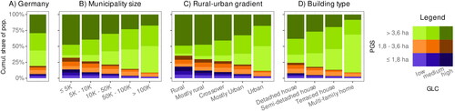
Therein, 80.8 % of people have access to 3.6 ha or more PGS in their neighbourhood, 12.6 % have between 1.8 and 3.6 ha, another 6.6 % have 1.8 ha or less PGS available. That is, 19.2 % of the population in Germany are underserved with regard to the goals set by the WHO.

Looking at the results by municipality size in Figure 2.B), it is clear that smaller municipalities generally feature higher amounts of GLC, as expressed by the larger share of darker shades. Conversely, the share of the population with access to more public green space increases with city size. While only two thirds of the population in small municipalities with less than 5,000 inhabitants have access to 3.6 ha of PGS or more, in cities with more than 100,000 inhabitants, this share increases to 91 %. This highlights that the importance of PGS as the primary resource for green space increases with municipality size.

The finer local resolution of the rural-urban gradient by Taubenböck et al. (2022), further underlines these results (cf. Figure 2.C)). Rural areas feature a majority of neighbourhoods with mid and high values of GLC, while 35.5 % of the population do not have enough PGS available in the neighbourhood. Conversely, 88.3 % of the population in urban centres have access to 3.6 ha and more.

GLC and PGS availability across neighbourhoods with different housing types in Figure 2.D) also reveals distinctive trends. More than half (61.5 %) of the population living in neighbourhoods with detached single-family, two-family homes or terraced houses find more than 25 ha of GLC in their neighbourhoods (medium and dark shades). In contrast, 24.5 % of the population in areas with detached homes find below-target PGS availability, 5.3 % more compared to entire Germany. Results for semi-detached house, terraced house and multi-family home areas show these areas increasingly feature less GLC and more PGS availability across the board.

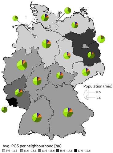
The map in Figure 3 illustrates the spatial distribution of green space availability throughout Germany. It shows the average amount of PGS for the population for each state which reveals that states with strong forest covers feature the highest average PGS for the population of the states of Saarland in the West and Brandenburg in the North-East. The highest share of the population with more than 3.6 ha PGS in the neighbourhood are the city states Berlin, Hamburg, and Bremen as well as the Saarland. Northern federal states, which characteristically feature more agricultural land and meadows show lower amounts of average PGS per neighbourhood and higher shares of the population with less than 3.6 ha of PGS in the neighbourhood.

Figure 3. Green space availability in Germany by federal states. States are shaded by the population-weighted average of PGS available. Pie charts indicate the distribution of PGS and GLC, the colors follow the legend in Figure 2.

4.2. Green space equity

Distributive equality of green space availability in Germany was assessed via the Gini coefficient. For all of Germany, the inequality of GLC availability is significantly lower (Gini = 0.32), than the inequality of PGS availability (Gini = 0.48, cf. Figure 4.A). This makes it clear that PGS is distributed much less fair throughout Germany.

Figure 4. Equity of GLC (pink) and PGS (green) availability in Germany at national, regional and city level. A) depicts a lorenz curve showing the availability of the resources in Germany. Point plots visualize the distribution of Gini coefficients measuring distributive equity of the resources in different spatial samples: B) by the municipality size denoted in classes of thousands (K) of inhabitants per municipality, C) by the neighbourhood classification along the rural-urban gradient, and D) by neighbourhoods with distinct housing types. For reference, the horizontal lines in B), C), and D) visualize the Gini coefficient per resource for the entire population of Germany.

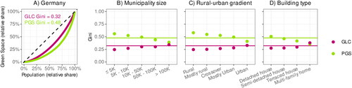
By comparing the Gini indices for GLC and PGS by the size of the municipality (cf. Figure 4.B), it is clear that the city size has an impact on the distributive equality of GLC and PGS. In fact, there exist inverse relationships for Gini indices between GLC and PGS. In case of major cities of more than 100,000 inhabitants, Gini coefficients for GLC and PGS reach comparable levels (Gini GLC 0.34, Gini PGS 0.39), while they diverge drastically for the population in municipalities with less than 5,000 inhabitants (Gini GLC 0.24, Gini PGS 0.56). In extension of the analysis by municipality size, Gini index results along the rural-urban gradient further highlight the inverse relationship between GLC and PGS inequality persists even with more local differentiation of urbanity (cf. Figure 4.C)).

The influence of the housing type on green space inequality shows clear trends, too. The inequality of GLC increases from areas with detached houses towards areas with multi-family homes. This trend is consistent with the previous results as multi-family dwellings are more common in denser urban centres. Remarkably, the inequality of the resource GLC (Gini = 0.38) exceeds the inequality of PGS (Gini = 0.35) in multi-family areas. This means that among all these neighbourhoods, the total available amount of GLC is less equally distributed among the population in these areas than the available PGS amount.

These results show that the inequality in neighbourhood GLC availability increases with city size, urbanity and more dense housing types. Conversely, along the same axes, the inequality in PGS availability decreases.

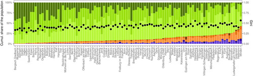
For the top 100 most populated cities in Germany the PGS availability and PGS Gini coefficients are compared (see Figure 5). Among these cities, above-target PGS coverages are recorded from almost 100 % of the population in Bergisch Gladbach to 55.3 % in Minden. Simultaneously, the PGS Gini coefficients for these cities do not reflect such a drastic trend. This highlights that while the Gini coefficient measures the distributive equality of green space amounts, it is not able to reflect which share of the population has access to sufficient green space amounts.

Figure 5. Comparison of green space availability by cumulative population share (coloured bars) and PGS Gini coefficient (black dots) for the 100 most populated cities in Germany. The colours follow the legend in Figure 2. The cities are ranked by the proportion of the population that has more than 3.6 hectares of the PGS in the neighbourhood which is the WHO target (green coloured bars). the main findings include: the range of population with above-target PGS values varies significantly among the largest cities, the PGS Gini coefficient only weakly correlates with the PGS above-target population shares (r = -0.52) with distinct outliers like darmstadt or heilbronn.

4.3. Green space availability and population composition

The relationship between green space availability and population composition across Germany to identify systemic differences for certain population groups was assessed using multiple LMM. In Table 2 the different models are summarized which utilize varying fixed effect variables and sets of random effect variables. Expectedly, all models show that GLC decreases most significantly with higher population, highlighting the importance of controlling for population density, which is a strong proxy for built-up density. In fact, an increase of the base 10 logarithm of the population by one, i.e. a 10-fold absolute increase, is associated with an average decrease of around 2.5 ha GLC (std. error 0.025 ha).

Table 2. LMM estimated fixed effects (FE) and random effects (RE) modelling the relation between green land cover (GLC, in ha.) and population (log.), the share of foreigners, children, and elderly across populated 1 km $\times$ 1 km grid cells in Germany.

	GLC (1)	GLC (2)	GLC (3)	GLC (4)	GLC (5)
Intercept FE	64.854^***	65.266^***	65.014^***	64.708^***	63.050^***
log(pop.) FE	−2.544^***	−2.766^***	−2.815^***	−2.754^***	−2.750^***
share foreign. FE	−0.195^***			−0.226^***	−0.224^***
share children FE		0.018^***		0.033^***	0.033^***
share elderly FE			0.042^***	0.041^***	0.041^***
Municip. RE	✓	✓	✓	✓	✓
City size class RE					✓
Rural-urban grad. RE
Model R^2	0.618	0.621	0.621	0.624	0.624
N cells	211,271	204,091	198,740	174,126	174,126
	GLC (6)	GLC (7)	GLC (8)	GLC (9)
Intercept FE	62.989^***	62.624^***	59.470^***	59.213^***
log(pop.) FE	−2.687^***	−2.688^***	−2.663^***	−2.530^***
share foreign. FE	−0.208^***	−0.208^***	−0.028^**	−0.003
share children FE	0.030^***	0.030^***	0.102^***	0.092^***
share elderly FE	0.040^***	0.040^***	0.069^***	0.066^***
Municip. RE	✓	✓
City size class RE		✓	✓
Rural-urban grad. RE	✓	✓		✓
Model R^2	0.626	0.626	0.050	0.053
N cells	174,091	174,091	174,126	174,091

Significance levels ^***p-value < 0.001,^**p-value < 0.01.

In terms of demographics, the models’ fixed effects consistently identify a lower amount of GLC as the share of foreigners in a neighbourhood increases, specifically −0.195 ha to −0.226 ha GLC per 1% increase. Conversely, both higher proportions of children and higher proportions of elderly in the neighbourhood are associated with higher amounts of GLC, albeit at lower magnitudes. By varying the included independent variables, we can see that the fixed effects are similar in all models. This shows that the different variables do indeed account for disjunct effects, which is further supported by generally low correlations between the fixed effects of neighbourhood demographics (correlation coefficients between −0.401 and 0.222 for GLC and −0.510 to 0.222 for PGS).

The impact of different random effect variables highlights the importance of the local geography and its influence on the GLC exposure of different population groups. This is visible through the difference of fixed effects of demographic composition variables between models with random effects by city size class or rural-urban gradient only (models 8 and 9) and models that include municipality random effects (models 1 - 7). The demographics’ fixed effects vary less between models with different demographic composition variables than when controlling for different random effects variables. Interestingly, models 8 and 9 report significantly lower coefficients of determination. Moreover, we see only marginal improvements of the models’ R² by controlling for random effects of the city size class and the rural-urban gradient in addition to municipality fixed effects (models 5 - 7).

Analogous to GLC, when estimating the relationship between PGS and neighbourhood demographics (see Table 3), it is found that PGS decreases most significantly with higher population density (log(pop.) FE). In contrast to GLC, the intercept for PGS is roughly half the magnitude. This is intuitive, as there are generally fewer hectares of PGS than GLC. Contrary to GLC, higher shares of children are associated with lower amounts of PGS (-0.074 - −0.0114), and neighbourhoods home to higher shares of foreigners feature more PGS availability (0.036 − 0.048). The latter is standing out as it marks the most significant and unexpected difference between the GLC and PGS models. The fixed effects across all variables are similar throughout all models.

Table 3. LMM estimated fixed effects (FE) and random effects (RE) modelling the relation between public green space (PGS, in ha.) and population (log.), the share of foreigners, children, and elderly across populated 1 km × 1 km grid cells in Germany.

	PGS (1)	PGS (2)	PGS (3)	PGS (4)	PGS (5)
Intercept FE	30.998^***	31.533^***	30.833^***	31.127^***	32.978^***
log(pop.) FE	−3.066^***	−2.888^***	−3.072^***	−2.877^***	−2.885^***
share foreign. FE	0.048^***			0.042^***	0.039^***
share children FE		−0.074^***		−0.082^***	−0.082^***
share elderly FE			0.021^***	0.018^***	0.017^***
Municip. RE	✓	✓	✓	✓	✓
City size class RE					✓
Rural-urban grad. RE
Model R ^2	0.456	0.459	0.457	0.455	0.455
N cells	211,271	204,091	198,740	174,126	174,126
	PGS (6)	PGS (7)	PGS (8)	PGS (9)
Intercept FE	31.835^***	32.809^***	30.775^***	30.520^***
log(pop.) FE	−2.896^***	−2.895^***	−2.519^***	−2.575^***
share foreign. FE	0.037^***	0.036^***	0.141^***	0.128^***
share children FE	−0.082^***	−0.082^***	−0.113^***	−0.114^***
share elderly FE	0.018^***	0.017^***	0.035^***	0.034^***
Municip. RE	✓	✓
City size class RE		✓	✓
Rural-urban grad. RE	✓	✓		✓
Model R ^2	0.455	0.455	0.067	0.069
N cells	174,091	174,091	174,126	174,091

Significance levels^***p-value < 0.001,^**p-value < 0.01.

Again, local conditions in individual cities and towns play an important role in the relationships between PGS and the independent variables. Similar to GLC, the model performance decreases when the random effects of the municipalities are excluded in models 8 and 9. These models also have quite different fixed effects than the models with municipality level random effects. Overall, the models show low correlations between the population share variables and most FE and RE show high significance (p-value < 0.001 (^***).

Creating individual models the classes of the rural-urban gradient, with random effects per municipality (cf. Tables 4 and 5) reveals notable variances in the magnitude of fixed effects between the rural-urban classes. In fact, for GLC the fixed effects of population density increases four-fold from rural to urban areas. This is not the case for PGS. The share of foreigners is positively related to GLC in rural areas (0.102 ^***), but negatively (−0.327^***) in urban areas. With some exceptions, the absolute effect sizes of the demographic compositions tend to increase towards more urban areas for GLC. This trend is not as pronounced for PGS. Coincidentally, the models’ R² decreases substantially with higher urbanity and the statistical significance, as measured by associated p-values, is partially lower compared to the global models. This indicates that the underlying systemic relations vary across different levels of urbanity.

Table 4. LMM estimated fixed effects (FE) and random effects (RE) modelling the relation between green land cover (GLC, in ha.) and population (log.), the share of foreigners, children, and elderly across populated 1 km × 1 km grid cells in Germany.

	GLC (1)	GLC (2)	GLC (3)	GLC (4)	GLC (5)
Intercept FE	59.726^***	63.079^***	62.946^***	64.989^***	63.731^***
log(pop.) FE	−1.176^***	−2.109^***	−2.646^***	−3.525^***	−4.783^***
share foreign. FE	0.102^***	−0.054^***	−0.137^***	−0.185^***	−0.327^***
share children FE	−0.011	−0.022^*	0.011	0.029^*	0.206^***
share elderly FE	0.017^**	0.015^**	0.052^***	0.065^***	0.255^***
Rural-urban class	Rural	Mostly rural	Crossover	Mostly Urban	Urban
Municip. RE	✓	✓	✓	✓	✓
Model R ^2	0.730	0.661	0.625	0.586	0.497
N cells	28,768	64,168	41,665	22,836	16,654

Significance levels^***p-value < 0.001,^**p-value < 0.01,^*p-value < 0.05.

Table 5. LMM estimated fixed effects (FE) and random effects (RE) modelling the relation between public green space (PGS, in ha.) and population (log.), the share of foreigners, children, and elderly across populated 1 km × 1 km grid cells in Germany.

	PGS (1)	PGS (2)	PGS (3)	PGS (4)	PGS (5)
Intercept FE	29.683^***	33.789^***	30.997^***	32.449^***	30.577^***
log(pop.) FE	−2.958^***	−3.336^***	−2.640^***	−2.538^***	−2.474^***
share foreign. FE	0.121^***	0.086^***	0.081^***	0.000	−0.016
share children FE	−0.032^***	−0.076^***	−0.077^***	−0.099^***	−0.067^***
share elderly FE	0.007	0.008.	0.038^***	0.025^**	0.108^***
Rural-urban class	Rural	Mostly rural	Crossover	Mostly Urban	Urban
Municip. RE	✓	✓	✓	✓	✓
Model R ^2	0.622	0.483	0.433	0.463	0.361
N cells	28,768	64,168	41,665	22,836	16,654

Significance levels^***p-value < 0.001,^**p-value < 0.01,^*p-value < 0.05,. p-value < 0.1.

5. Discussion

In this study, we utilized vast geographic data to quantify available green land cover (GLC) and public green space (PGS) on neighbourhood scale for an entire nation. We aimed at (1) analysing how GLC and PGS are distributed among the German population, (2) quantifying how many people have access to sufficient levels of PGS and how this contrasts with GLC and (3) identifying how different neighbourhood demographics relate to green space availability.

5.1. Green space availability in Germany

We derived green space availability for Germany’s entire population from satellite imagery, land cover information, open geographic data, and machine learning. To our knowledge, this is the first study to investigate the availability of public green spaces nationwide on a local level. We quantified the availability of green land cover and publicly accessible green spaces in the neighbourhoods of people in Germany. In line with the existing literature (e.g. de Voorde 2017), a weak correlation between PGS and GLC (r = 0.617) highlights the importance of analysing different green types. Previous studies were limited to single cities or EUA areas; we expanded the extent in this study by modelling PGS using a data fusion model incorporating vast satellite imagery and VGI data. The methodology for data acquisition used in this study helped us to alleviate these limitations and enabled an analysis of public green spaces independent of arbitrary data boundaries posed by EUA extents.

The nationwide analysis showed that the majority of the German population has more PGS than the minimum defined by the WHO (RQ1). Especially in rural regions, however, the share of people meeting these targets decreases significantly. Also, across different cities and federal states, we found high variations. This further adds to the findings of Taubenböck et al. (2021) emphasizing that the diversity of the local landscape plays a major role in the amount of green spaces in a city. The present study, however, adds two perspectives: First, it assesses different types of green, specifically publicly available green spaces. And second, it conducts a high-resolution, national scale analysis of the available green space including the entire population in Germany.

Our analysis revealed significant differences between neighbourhood green space availability in urban and rural regions both by its available amount but also the distributive equality among the population. The results showed public green is an important resource especially in densely urbanized regions. However, also in cities, high amounts of GLC did not necessarily equate to high amounts of PGS. Neighbourhoods with predominantly detached houses and semi-detached houses might have higher GLC availability but above-target PGS availability is still lower than in more densely populated areas with multi-family homes.

Similarly, rural regions are more likely to have sub-target public green space availabilities. Similar disparities can be expected for other health relevant amenities, too (Pearce et al. 2006). Furthermore, public green spaces in the rural regions are more likely to be natural environments and have been shown to have greater impact on health (Wheeler et al. 2015). Arguably, which green spaces can be found in the neighbourhood, depends strongly on individual perception. In rural areas, people might live far away from any park, but are able to take a walk in the fields and nearby forests. It is therefore necessary to analyse pathways as a function of urbanity and assess possibly differing health implications of salutogenic resources across different regimes. After all, previous studies have indicated that the access and exposure to green spaces are only weakly correlated (Jarvis et al. 2020). Our study does not evaluate the objective and subjective importance of publicly accessible green spaces, but provides a data basis and a methodological approach to support such studies; future research should evaluate how the rural population uses and values PGS and how this differs from urban dwellers. This extends to any socioeconomic confounders, as it has been found that social status significantly impacts the use, relevance, and impact of green spaces on health (Kabisch 2019; Rehling et al. 2021). The data used in this study provide limited scope to account for such confounding influences.

5.2. Demographic equity of green space availability in Germany

The most important finding of this study is that there is a significant difference in distributive equity depending on the type of green space taken into account (cf. RQ2). In all but one evaluation using the Gini coefficient, GLC availability was more equally distributed across the population than PGS. This indicates that the resource public green is more concentrated and thus more disproportionately distributed among the German population than GLC. As discussed by de Voorde (2017), this highlights the relevance of incorporating the type and accessibility of green spaces into urban planning since GLC as reference metric for green cover might overestimate the availability of usable green spaces and underestimate disproportionate access for certain populations.

Further, diverging trends of Gini coefficients between the two green space types availabilities accentuate the stark differences between rural and urban areas. This highlights the diversity of green space availabilities and the necessity for localized assessment of green space resources. Regional differences are strongly dependent on the local geographic setting such as the degree of urbanization. This study also stresses that PGS inequality is especially high in rural regions. There, the disparity of public green availability is increased on the one hand by private gardens and agricultural areas, and on the other hand by homes close to larger forests.

However, comparing Gini coefficients among different populations must be interpreted with care; it refers to different total amounts of available resources. It only describes the distribution of the available amount. Our result of the top 100 most populated cities in Germany showed that the Gini coefficient does not provide conclusive data on which share of the population might be underserved with public green. Also, outside urban areas, the relevance of PGS as the main source of green space in the environment might diminish. While the park might be the most important source of public green in the city, in rural areas, other and more diverse forms of green, such as meadows or fields, are more relevant to the people. Our assumption in the data model is not able to reflect these subjective differences in preference.

Put differently, the higher availability of PGS in larger cities can also be seen as testament of targeted urban planning. Where GLC is less prevalent by design due to increasing built-up density, the importance of PGS provision for the urban population excels. Where there is no space for everybody to have a private garden, the share of people having access to sufficient PGS is higher.

The relationship between demographic composition and neighbourhood green space availability addresses inequities in relation to different demographic characteristics (see RQ3). While an increasing share of foreign population in the neighbourhood is associated with a decrease in GLC, this trend is inverse for PGS. This aligns with the majority of the foreign population living in cities and similar result found by Barbosa et al. (2007) for the United Kingdom. However, the difference in magnitude between the two effects shows that the reduction in GLC is not fully compensated for by an equal increase in PGS. Thus, neighbourhoods with a higher share of immigrants are generally more disadvantaged in terms of benefits of GLC, e.g. ambient cooling (Park et al. 2017). It further highlights that PGS is an especially important source for green space in these neighbourhoods.

In contrast, the relations between the availability of GLC and neighbourhoods with higher shares of children as well as higher shares of older people were much less clear. This can be interpreted as an indication that systemic inequality is more pronounced for neighbourhoods with higher proportions of foreign population. The small positive association between the share of children and GLC and its small negative association with PGS can be indicative of the suburbanization movement of young families who move to the suburbs with higher amounts of private green as opposed to public parks. Still, without more detailed socioeconomic data allowing to account for other confounding factors, no conclusive findings can be drawn.

The effects of different compositions of population share effects were stable while controlling for population, indicating independent effects. This holds true across experiments with different fixed effects groups. The model performance (measured by R²) was highest when controlling for city random effects. This indicates that local phenomena indeed have a strong influence on the relation between green space availability and population composition. Intercepts and effects of (log.) population stayed stable across different variable combinations, indicating strong independence from population shares and random effects variables.

5.3. Limitations and future research

This study uses green space availability in the neighbourhood as a key metric. This, however, does not necessarily reflect how accessible these areas are for the people. We estimated the available PGS in a rectangular neighbourhood enclosing a 500 m buffer, driven by the input to the PGS model. While the exact distance was based on the literature, a wide range of neighbourhood definitions exist as discussed by Kabisch (2019). Beyond that, target indicator evaluation of SDG 11.7 calls for an assessment of all green spaces within 400 m walking distance.⁵ This is why PGS availability could additionally be combined with concepts like individual walkable neighbourhoods (Droin et al. 2023) to increase the level of detail and thus relate more to the realistic experience of pedestrians, possibly accounting for different walking speeds. Extending the analyses to further include the environment around the individuals’ places of work (e.g. Rauch et al. 2021) would allow creating a more differentiated picture of the distribution of GS accessibility. Also, for example, health implications related to green space have been shown to depend on the size of the neighbourhood (Reid et al. 2018; Su et al. 2019), limiting our study to effects underlying the modifiable areal units problem (MAUP). As this was out of the scope of this study, we focused on distances derived from literature. To identify possible pathways of PGS on health, multiple neighbourhood extents, possibly in combination with the walkability of the neighbourhood would have to be taken into account. This warrants to expand future studies to explore the impact of different sized neighbourhoods.

We based our green space type PGS on EUA data, which has shown high accuracy for urban green space (Liao et al. 2021). As Kabisch et al. (2016) discussed, these have some inherent data limitations in that they define classes rather broadly. Taking the example of Green urban areas, they comprise multiple diverse urban green classes. Also, the minimum mapping unit of 0.25 ha per object may obscure smaller green space features in complex urban settings. To account for a more diverse set of urban green space types, the data fusion approach used in this study could be extended to more explicit and complex green space ontologies (e.g. Ismayilova and Timpf 2022). Although the data fusion based methodology was specifically chosen to reduce the impact related to errors, omissions or incorrectly tagged OSM features (cf. Dorn et al. 2015), we acknowledge that the results are heavily dependent on the quality of the used VGI data. In Germany and Europe VGI quality is comparably high, which is why the applicability of this method might be subject to local restrictions. Further research is required to scrutinize the applicability of modelling PGS across different regions or continents. Similar to the impact of OSM data quality, the classification scheme of the Sentinel-2 based land cover classification as proposed by Weigand et al. (2020) may introduce bias. Therefore, we want to acknowledge that recently different large scale land cover products were made available that could be utilized for similar analyses, for example Dynamic World (Brown et al. 2022) or ESA World Cover.⁶

We used the most recent census data in Germany dating back to 2011. More up-to-date data were unavailable due to delays caused by the COVID-19 pandemic⁷. Additionally, the spatial grid format induces some limitations to this study. Firstly, it does not allow for detailed description of individuals by means of multiple socioeconomic variables, i.e. migration background and education and income and age. Therefore, it was infeasible to control for confounding socioeconomic variables in this study. This would be possible with more detailed socioeconomic survey data (e.g. Krekel et al. 2016; Wüstemann et al. 2017). Secondly, randomization effects introduce bias in sparsely populated cells. Naturally, these cells are more likely to occur in less populated areas, which is likely to be the case in rural areas or in the outskirts of cities. This can impact this study as we tend to underestimate the share of people in regions with lower population density and possibly high GLC/PGS availability. When extending similar studies to broader international or global contexts, national census data could hinder scalability. In these cases, global population datasets, e.g. WorldPop (Tatem 2017), could provide consistent large-scale demographic data as demonstrated by Long et al. (2022).

Even though administrative boundaries were used to distinguish different cities and their population, they do not necessarily reflect reality in terms of urban regions (Taubenböck et al. 2019). It would therefore be interesting to investigate the influence of morphological urban regions on the availability of green spaces.

6. Conclusions

In this study, we have demonstrated how publicly available geographic data can be utilized to enable analyses of social equity of GS availability on a nationwide level. Therein, we highlighted the differences between two representations of green space: green land cover (GLC) and public green space (PGS). Despite the large area under investigation, these data allowed for a high spatial resolution and consistency. With this, it was possible to analyse the green space availability on the level of neighbourhoods. In combination with census data we were able to quantify the distribution of green space availability among the population and its relation to societal composition. This shows that modern geographic data can provide vital information to facilitate nationwide analyses of social equity or environmental justice. We thus closed previously identified gaps for semantically diverse and spatially detailed, exhaustive data.

Overall, more than 80 % of the German population have access to more PGS than defined by the WHO target. We found that both GLC and PGS availability vary significantly by the degree urbanity and correlate with the building structure in the neighbourhood. These two resources are distributed very differently among the population, even showing opposing trends along the rural-urban gradient. Neighbourhoods with larger shares of foreign inhabitants experience lower amounts of GLC, a trend that cannot be found for PGS in Germany.

Future research is suggested to increase the semantic depth of the analysis to identify more diverse patterns of green space availability among the population. Combining nationwide neighbourhood green space type data with panel data and more detailed socioeconomic information can help identify further social inequalities with regard to green spaces in Germany. Paired with health records, the fusion of geographic data can be used better identify health implications and pathways of exposure or access to various green space types.

Acknowledgements

The authors acknowledge the data provided by the OpenStreetMap project and its contributors under the terms of the Open Data Commons Open Database License (ODbL). The authors thank two anonymous reviewers for their helpful comments and suggestions.

Disclosure statement

No potential conflict of interest was reported by the author(s).

Data availability statement

Data available from the authors on request. The code used for this study is published at https://github.com/dlr-eoc/ukis-paperfairgreen.

Additional information

Funding

This study was partly funded by the German Federal Environmental Foundation (DBU). The funding sponsors had no role in the study design, interpretation, manuscript writing, or publishing decision.

Notes

1 https://ec.europa.eu/eurostat/web/lucas/overview (accessed 2023-03-24)

2 https://land.copernicus.eu/local/urban-atlas (accessed 2023-03-24)

3 The software for this study was implemented in Python 3.9.6 and TensorFlow 2.8.

4 https://www.zensus2011.de/DE/Home/Aktuelles/DemografischeGrunddaten.html

5 https://unstats.un.org/sdgs/metadata/files/Metadata-11-07-01.pdf

6 https://esa-worldcover.org

7 https://www.zensus2022.de/DE/Aktuelles/verschiebung\_beschluss.html

References

- Akpinar A, Barbosa-Leiker C, Brooks KR. 2016. Does green space matter? Exploring relationships between green space type and health indicators. Urban For Urban Green. 20:407–418. doi: 10.1016/j.ufug.2016.10.013.
- Artmann M, Mueller C, Goetzlich L, Hof A. 2019. Supply and demand concerning urban green spaces for recreation by elderlies living in care facilities: the role of accessibility in an explorative case study in austria. Front Environ Sci. 7:12. doi: 10.3389/fenvs.2019.00136.
- Barber A, Haase D, Wolff M. 2021. Permeability of the city – physical barriers of and in urban green spaces in the city of Halle, Germany. Ecol Indic. 125(107555):107555. doi: 10.1016/j.ecolind.2021.107555.
- Barbosa O, Tratalos JA, Armsworth PR, Davies RG, Fuller RA, Johnson P, Gaston KJ. 2007. Who benefits from access to green space? a case study from Sheffield, UK. Landscape Urban Plann. 83(2-3):187–195. doi: 10.1016/j.landurbplan.2007.04.004.
- Berdejo-Espinola V, Suárez-Castro AF, Amano T, Fielding KS, Oh RRY, Fuller RA. 2021. Urban green space use during a time of stress: a case study during the COVID-19 pandemic in Brisbane, Australia. People Nat (Hoboken). 3(3):597–609. doi: 10.1002/pan3.10218.
- Brown CF, Brumby SP, Guzder-Williams B, Birch T, Hyde SB, Mazzariello J, Czerwinski W, Pasquarella VJ, Haertel R, Ilyushchenko S, et al. 2022. Dynamic world, near real-time global 10 m land use land cover mapping. Sci Data. 9(1):17. doi: 10.1038/s41597-022-01307-4.
- Castelli C, d’Hombres B, de Dominicis L, Dijkstra L, Montalto V, Pontarollo N. 2023. What makes cities happy? Factors contributing to life satisfaction in European cities. Eur Urban Reg Stud. 30(4):319–342. doi: 10.1177/09697764231155335.
- de Voorde TV. 2017. Spatially explicit urban green indicators for characterizing vegetation cover and public green space proximity: a case study on Brussels, Belgium. Int J Digital Earth. 10(8):798–813.
- Dewulf B, Neutens T, Van Dyck D, De Bourdeaudhuij I, Broekx S, Beckx C, Van de Weghe N. 2016. Associations between time spent in green areas and physical activity among late middle-aged adults. Geospat Health. 11(3):411. doi: 10.4081/gh.2016.411.
- Dorn H, Törnros T, Zipf A. 2015. Quality evaluation of VGI using authoritative data—a comparison with land use data in southern Germany. IJGI. 4(3):1657–1671. doi: 10.3390/ijgi4031657.
- Droin A, Wurm M, Taubenböck H. 2023. The individual walkable neighborhood - evaluating people-centered spatial units focusing on urban density. Comput Environ Urban Syst. 99:101893. doi: 10.1016/j.compenvurbsys.2022.101893.
- Enssle F, Kabisch N. 2020. Urban green spaces for the social interaction, health and well-being of older people—an integrated view of urban ecosystem services and socio-environmental justice. Environ Sci Policy. 109:36–44. doi: 10.1016/j.envsci.2020.04.008.
- Feltynowski M, Kronenberg J, Bergier T, Kabisch N, Łaszkiewicz E, Strohbach MW. 2018. Challenges of urban green space management in the face of using inadequate data. Urban For Urban Green. 31:56–66. doi: 10.1016/j.ufug.2017.12.003.
- Flacke J, Schüle SA, Köckler H, Bolte G. 2016. Mapping environmental inequalities relevant for health for informing urban planning interventions – a case study in the city of Dortmund, Germany. Int J Environ Res Public Health. 13(7):711. doi: 10.3390/ijerph13070711.
- Fukushima K. 1969. Visual feature extraction by a multilayered network of analog threshold elements. IEEE Trans Syst Sci Cyber. 5(4):322–333. doi: 10.1109/TSSC.1969.300225.
- Georganos S, Hafner S, Kuffer M, Linard C, Ban Y. 2022. A census from heaven: unraveling the potential of deep learning and earth observation for intra-urban population mapping in data scarce environments. Int J Appl Earth Obs Geoinf. 114:103013. doi: 10.1016/j.jag.2022.103013.
- Gómez-Baggethun E, Gren Å, Barton DN, Langemeyer J, McPhearson T, O’Farrell P, Andersson E, Hamstead Z, Kremer P. 2013. Urban ecosystem services. In Elmqvist, T., Fragkais, M., Goodness, J., Güneralp, B., Marcotullio, P. J., McDonald, R. I., Parnell, S., Schewenius, M., Sendstad, M., Seto, K. C., and Wilkinson, C., editors, Urbanization, biodiversity and ecosystem services: challenges and opportunities, 175–251. Dodrecht: Springer Netherlands.
- Goodfellow I, Bengio Y, Courville A. 2016. Deep learning. Cambridge, MA: MIT Press.
- Honold J, Lakes T, Beyer R, van der Meer E. 2016. Restoration in urban spaces: nature views from home, greenways, and public parks. Environ Behav. 48(6):796–825. doi: 10.1177/0013916514568556.
- Hunter AJ, Luck GW. 2015. Defining and measuring the social-ecological quality of urban greenspace: a semi-systematic review. Urban Ecosyst. 18(4):1139–1163. doi: 10.1007/s11252-015-0456-6.
- Ioffe S, Szegedy C. 2015. Batch normalization: accelerating deep network training by reducing internal covariate shift. In Proceedings of the 32nd International Conference on Machine Learning, p. 448–456. PMLR.
- Ismayilova I, Timpf S. 2022. Towards an ontology of urban green spaces. GI_Forum. 2022(2):47–57.
- Jarvis I, Gergel S, Koehoorn M, van den Bosch M. 2020. Greenspace access does not correspond to nature exposure: measures of urban natural space with implications for health research. Landscape Urban Plann. 194:103686. doi: 10.1016/j.landurbplan.2019.103686.
- Jennings V, Gaither CJ, Gragg RS. 2012. Promoting environmental justice through urban green space access: a synopsis. Environ Justice. 5(1):1–7. doi: 10.1089/env.2011.0007.
- Jim CY, Chen WY. 2006. Perception and attitude of residents toward urban green spaces in Guangzhou (China). Environ Manage. 38(3):338–349. doi: 10.1007/s00267-005-0166-6.
- Jimenez RB, Lane KJ, Hutyra LR, Fabian MP. 2022. Spatial resolution of normalized difference vegetation index and greenness exposure misclassification in an urban cohort. J Expo Sci Environ Epidemiol. 32(2):213–222. doi: 10.1038/s41370-022-00409-w.
- Jünger S. 2021. Land use disadvantages in Germany: a matter of ethnic income inequalities? Urban Stud. 59(9):1819–1836. doi: 10.1177/00420980211023206.
- Jorgensen A, Gobster PH. 2010. Shades of green: measuring the ecology of urban green space in the context of human health and well-being. Nat Cult. 5(3):338–363. doi: 10.3167/nc.2010.050307.
- Kabisch N. 2019. The influence of socio-economic and socio-demographic factors in the association between urban green space and health. In Marselle, M. R., Stadler, J., Korn, H., Irvine, K. N., and Bonn, A., editors, Biodiversity and health in the face of climate change, p. 91–119. Cham: Springer International Publishing.
- Kabisch N, Haase D. 2014. Green justice or just green? Provision of urban green spaces in Berlin, Germany. Landscape Urban Plann. 122:129–139. doi: 10.1016/j.landurbplan.2013.11.016.
- Kabisch N, Strohbach M, Haase D, Kronenberg J. 2016. Urban green space availability in European cities. Ecol Indic. 70:586–596. doi: 10.1016/j.ecolind.2016.02.029.
- Klompmaker JO, Hoek G, Bloemsma LD, Gehring U, Strak M, Wijga AH, van den Brink C, Brunekreef B, Lebret E, Janssen NA. 2018. Green space definition affects associations of green space with overweight and physical activity. Environ Res. 160:531–540. doi: 10.1016/j.envres.2017.10.027.
- Krekel C, Kolbe J, Wüstemann H. 2016. The greener, the happier? the effect of urban land use on residential well-being. Ecol Econ. 121:117–127. doi: 10.1016/j.ecolecon.2015.11.005.
- Lee ACK, Maheswaran R. 2011. The health benefits of urban green spaces: a review of the evidence. J Public Health (Oxf). 33(2):212–222. doi: 10.1093/pubmed/fdq068.
- Liao Y, Zhou Q, Jing X. 2021. A comparison of global and regional open datasets for urban greenspace mapping. Urban For Urban Green. 62:127132. doi: 10.1016/j.ufug.2021.127132.
- Lin BB, Fuller RA, Bush R, Gaston KJ, Shanahan DF. 2014. Opportunity or orientation? Who uses urban parks and why. PLoS One. 9(1):e87422. doi: 10.1371/journal.pone.0087422.
- Long X, Chen Y, Zhang Y, Zhou Q. 2022. Visualizing green space accessibility for more than 4,000 cities across the globe. Environ Plann B: Urban Analyt City Sci. 49(5):1578–1581. doi: 10.1177/23998083221097110.
- Ludwig C, Hecht R, Lautenbach S, Schorcht M, Zipf A. 2021. Mapping public urban green spaces based on OpenStreetMap and sentinel-2 imagery using belief functions. IJGI. 10(4):251. doi: 10.3390/ijgi10040251.
- Maas J, Verheij RA, Groenewegen PP, De Vries S, Spreeuwenberg P. 2006. Green space, urbanity, and health: how strong is the relation? J Epidemiol Community Health. 60(7):587–592. doi: 10.1136/jech.2005.043125.
- Mears M, Brindley P, Jorgensen A, Maheswaran R. 2020. Population-level linkages between urban greenspace and health inequality: the case for using multiple indicators of neighbourhood greenspace. Health Place. 62(:102284. doi: 10.1016/j.healthplace.2020.102284.
- Middel A, Häb K, Brazel AJ, Martin CA, Guhathakurta S. 2014. Impact of urban form and design on mid-afternoon microclimate in Phoenix Local Climate Zones. Landscape Urban Plann. 122:16–28. doi: 10.1016/j.landurbplan.2013.11.004.
- Openshaw S. 1983. The modifiable areal unit problem. Number 38 in Concepts and techniques in modern geography. Norwich, England: Geo Books.
- Park J, Kim J-H, Lee DK, Park CY, Jeong SG. 2017. The influence of small green space type and structure at the street level on urban heat island mitigation. Urban For Urban Green. 21:203–212. doi: 10.1016/j.ufug.2016.12.005.
- Pearce J, Witten K, Bartie P. 2006. Neighbourhoods and health: a GIS approach to measuring community resource accessibility. J Epidemiol Community Health. 60(5):389–395. doi: 10.1136/jech.2005.043281.
- Pflugmacher D, Rabe A, Peters M, Hostert P. 2019. Mapping pan-European land cover using Landsat spectral-temporal metrics and the European LUCAS survey. Remote Sens Environ. 221:583–595. doi: 10.1016/j.rse.2018.12.001.
- Poortinga W, Bird N, Hallingberg B, Phillips R, Williams D. 2021. The role of perceived public and private green space in subjective health and wellbeing during and after the first peak of the COVID-19 outbreak. Landsc Urban Plan. 211:104092. doi: 10.1016/j.landurbplan.2021.104092.
- Pope D, Tisdall R, Middleton J, Verma A, van Ameijden E, Birt C, Macherianakis A, Bruce N. 2015. Quality of and access to green space in relation to psychological distress: results from a population-based cross-sectional study as part of the EURO-URHIS 2 project. Eur J Public Health. 28(1):35–38. doi: 10.1093/eurpub/ckv094.
- Pugh TAM, MacKenzie AR, Whyatt JD, Hewitt CN. 2012. Effectiveness of green infrastructure for improvement of air quality in urban street canyons. Environ Sci Technol. 46(14):7692–7699. doi: 10.1021/es300826w.
- Qiu C, Tong X, Schmitt M, Bechtel B, Zhu XX. 2020. Multilevel feature fusion-based CNN for local climate zone classification from sentinel-2 images: benchmark results on the so2sat LCZ42 dataset. IEEE J Sel Top Appl Earth Observ Remote Sens. 13:2793–2806. doi: 10.1109/JSTARS.2020.2995711.
- Rauch S, Taubenböck H, Knopp C, Rauh J. 2021. Risk and space: modelling the accessibility of stroke centers using day- & nighttime population distribution and different transportation scenarios. Int J Health Geogr. 20(1):31. doi: 10.1186/s12942-021-00284-y.
- Rehling J, Bunge C, Waldhauer J, Conrad A. 2021. Socioeconomic differences in walking time of children and adolescents to public green spaces in urban areas—results of the german environmental survey (2014–2017). Int J Environ Res Public Health. 18(5):2326. doi: 10.3390/ijerph18052326.
- Reid CE, Kubzansky LD, Li J, Shmool JL, Clougherty JE. 2018. It’s not easy assessing greenness: a comparison of NDVI datasets and neighborhood types and their associations with self-rated health in New York City. Health Place. 54:92–101. doi: 10.1016/j.healthplace.2018.09.005.
- Richardson E, Pearce J, Mitchell R, Kingham S. 2013. Role of physical activity in the relationship between urban green space and health. Public Health. 127(4):318–324. doi: 10.1016/j.puhe.2013.01.004.
- Rigolon A. 2016. A complex landscape of inequity in access to urban parks: a literature review. Landscape Urban Plann. 153:160–169. doi: 10.1016/j.landurbplan.2016.05.017.
- Rosier JF, Taubenböck H, Verburg PH, van Vliet J. 2022. Fusing earth observation and socioeconomic data to increase the transferability of large-scale urban land use classification. Remote Sens Environ. 278:113076. doi: 10.1016/j.rse.2022.113076.
- Russette H, Graham J, Holden Z, Semmens EO, Williams E, Landguth EL. 2021. Greenspace exposure and COVID-19 mortality in the United States: January–July 2020. Environ Res. 198:111195. doi: 10.1016/j.envres.2021.111195.
- Santos T, Tenedório J, Gonçalves J. 2016. Quantifying the city’s green area potential gain using remote sensing data. Sustainability. 8(12):1247. doi: 10.3390/su8121247.
- Sapena M, Wurm M, Taubenböck H, Tuia D, Ruiz LA. 2021. Estimating quality of life dimensions from urban spatial pattern metrics. Comput Environ Urban Syst. 85(:101549. doi: 10.1016/j.compenvurbsys.2020.101549.
- Schüle SA, Hilz LK, Dreger S, Bolte G. 2019. Social inequalities in environmental resources of green and blue spaces: a review of evidence in the WHO European region. Int J Environ Res Public Health. 16(7):1216. doi: 10.3390/ijerph16071216.
- Su JG, Dadvand P, Nieuwenhuijsen MJ, Bartoll X, Jerrett M. 2019. Associations of green space metrics with health and behavior outcomes at different buffer sizes and remote sensing sensor resolutions. Environ Int. 126:162–170. doi: 10.1016/j.envint.2019.02.008.
- Swanwick C, Dunnett N, Woolley H. 2003. Nature, role and value of green space in towns and cities: an overview. Built Environ. 29(2):94–106. doi: 10.2148/benv.29.2.94.54467.
- Tatem AJ. 2017. WorldPop, open data for spatial demography. Sci Data. 4(1):170004. doi: 10.1038/sdata.2017.4.
- Taubenböck H, Droin A, Standfuß I, Dosch F, Sander N, Milbert A, Eichfuss S, Wurm M. 2022. To be, or not to be ‘urban’? A multi-modal method for the differentiated measurement of the degree of urbanization. Comput Environ Urban Syst. 95:101830. doi: 10.1016/j.compenvurbsys.2022.101830.
- Taubenböck H, Reiter M, Dosch F, Leichtle T, Weigand M, Wurm M. 2021. Which city is the greenest? A multi-dimensional deconstruction of city rankings. Comput Environ Urban Syst. 89:101687. doi: 10.1016/j.compenvurbsys.2021.101687.
- Taubenböck H, Weigand M, Esch T, Staab J, Wurm M, Mast J, Dech S. 2019. A new ranking of the world’s largest cities—Do administrative units obscure morphological realities? Remote Sens Environ. 232:111353 doi: 10.1016/j.rse.2019.111353.
- Taylor L, Hochuli DF. 2017. Defining greenspace: multiple uses across multiple disciplines. Landscape Urban Plann. 158:25–38. doi: 10.1016/j.landurbplan.2016.09.024.
- UN General Assembly. 2015. Transforming our world: the 2030 agenda for sustainable development. Technical report, A/RES/70/1, 21 October 2015.
- Vargas-Munoz JE, Srivastava S, Tuia D, Falcao AX. 2021. OpenStreetMap: challenges and opportunities in machine learning and remote sensing. IEEE Geosci Remote Sens Mag. 9(1):184–199. doi: 10.1109/MGRS.2020.2994107.
- Villeneuve PJ, Jerrett M, Su JG, Burnett RT, Chen H, Wheeler AJ, Goldberg MS. 2012. A cohort study relating urban green space with mortality in Ontario, Canada. Environ Res. 115:51–58. doi: 10.1016/j.envres.2012.03.003.
- Weigand M, Staab J, Wurm M, Taubenböck H. 2020. Spatial and semantic effects of LUCAS samples on fully automated land use/land cover classification in high-resolution Sentinel-2 data. Int J Appl Earth Obs Geoinf. 88(:102065. doi: 10.1016/j.jag.2020.102065.
- Weigand M, Wurm M, Dech S, Taubenböck H. 2019. Remote sensing in environmental justice research – a review. IJGI. 8(1):20. doi: 10.3390/ijgi8010020.
- Wheeler BW, Lovell R, Higgins SL, White MP, Alcock I, Osborne NJ, Husk K, Sabel CE, Depledge MH. 2015. Beyond greenspace: an ecological study of population general health and indicators of natural environment type and quality. Int J Health Geogr. 14(1):17. (doi: 10.1186/s12942-015-0009-5.
- Wolff M, Haase D. 2019. Mediating sustainability and liveability—turning points of green space supply in European cities. Front Environ Sci. 7, 1–14. doi: 10.3389/fenvs.2019.00061.
- World Health Organization. 2017. Urban green spaces: a brief for action. Copenhagen, Denmark: World Health Organization. Regional Office for Europe.
- World Health Organization. 2020. Mental health and psychosocial considerations during the covid-19 outbreak. https://www.who.int/docs/default-source/coronaviruse/mental-health-considerations.pdf.
- Wüstemann H, Kalisch D, Kolbe J. 2017. Accessibility of urban blue in German major cities. Ecol Indic. 78:125–130. doi: 10.1016/j.ecolind.2017.02.035.
- Wurm M, Goebel J, Wagner GG, Weigand M, Dech S, Taubenböck H. 2019a. Inferring floor area ratio thresholds for the delineation of city centers based on cognitive perception. Environ Plann B: urban Analyt City Sci. 48(2):265–279. doi: 10.1177/2399808319869341.
- Wurm M, Stark T, Zhu XX, Weigand M, Taubenböck H. 2019b. Semantic segmentation of slums in satellite images using transfer learning on fully convolutional neural networks. ISPRS J Photogramm Remote Sens. 150:59–69. doi: 10.1016/j.isprsjprs.2019.02.006.
- Wurm M, Weigand M, Stark T, Goebel J, Wagner GG, Taubenböck H. 2019c. Modelling the impact of the urban spatial structure on the choice of residential location using ‘big earth data’ and machine learning. In 2019 Joint Urban Remote Sensing Event (JURSE). IEEE. doi: 10.1109/JURSE.2019.8808942.
- Wüstemann H, Kalisch D, Kolbe J. 2017. Access to urban green space and environmental inequalities in Germany. Landscape Urban Plann. 164:124–131. doi: 10.1016/j.landurbplan.2017.04.002.
- Xu C, Haase D, Pauleit S. 2018a. The impact of different urban dynamics on green space availability: a multiple scenario modeling approach for the region of Munich, Germany. Ecol Indic. 93:1–12. doi: 10.1016/j.ecolind.2018.04.058.
- Xu C, Haase D, Pribadi DO, Pauleit S. 2018b. Spatial variation of green space equity and its relation with urban dynamics: a case study in the region of Munich. Ecol Indic. 93:512–523. doi: 10.1016/j.ecolind.2018.05.024.
- Zepp H, Groß L, Inostroza L. 2020. And the winner is? Comparing urban green space provision and accessibility in eight European metropolitan areas using a spatially explicit approach. Urban Forestry & Urban Greening. 49(:126603. doi: 10.1016/j.ufug.2020.126603.
- Zhuang S, Bolte G, Lakes T. 2022. Exploring environmental health inequalities: a scientometric analysis of global research trends (1970–2020). Int J Environ Res Public Health. 19(12):7394. doi: 10.3390/ijerph19127394.
- Zuniga-Teran A, Gerlak A. 2019. A multidisciplinary approach to analyzing questions of justice issues in urban greenspace. Sustainability. 11(11):3055. doi: 10.3390/su11113055.