Past and future land use/land cover, and climate change impacts on environmental sustainability in Vea catchment, Ghana

Abstract

LULC and climate change are the two most common manifestations of global environmental change. The objective of this study was to quantify past and future LULC and climate change impacts on environmental sustainability in the Vea catchment of Ghana. The past LULC change (1998–2022) was analyzed using ERDAS Imagine 15 upon the application of the Support Vector Machine (SVM) classifier algorithm. The CA-Markov was used to predict land-use changes in 2038 and 2054. Climate change was projected under SSP 4.5 and SSP 8.5 emission scenarios using the R software. The projections from an ensemble mean of SSPs in the near future (2023–2052) and far future (2071–2100) were compared to the reference period (1993–2022). The results show that, between 1998 and 2022, cropland increased from 10.9% to 51.98%, while grassland and forest areas decreased from 54.8–18.14% and 31.7–22.73%, respectively. The results of the predicted LULC change showed an increase in cropland from 181 km² in 2038 to 183 km² in 2054 at the expense of grassland and forest, which are expected to decrease from 51–50 km² and 73–71 km², respectively. The findings of climate change show the projected increases in average temperature range from 2.10 to 3.5 °C under SSP4.5 and from 2.7 to 4.15 °C under SSP8.5. Under the SSP4.5, annual average precipitation is anticipated to decrease by 12.34–13.1%, while the SSP8.5 projects a decrease of 12.6–13.6%. Results will help in the setting up of long-term environmental management strategies in the catchment as well as the development of appropriate adaptation methods to mitigate the ongoing impacts of LULC and climate change on environmental sustainability.

Keywords:

• Geospatial technique
• LULC
• climate change
• CA-Markov
• SSPs
• Ghana

1. Introduction

Land use/land cover and climate change are the two most common manifestations of global environmental change Hassan et al. (2016); Koko et al. (2022). ‘Land use’ and ‘land cover’ describe the complex interactions between man and the physical environment (Wang J et al. 2022). Land use (LU) is the result of anthropogenic changes to the land surface, such as agriculture, forestry, and construction. Land cover (LC) describes the morphological and living features on the land’s surface, including wetlands, vegetation, reservoirs, and artificial structures (Liu et al. 2021). Climate change is defined as a statistically significant shift in the average climatic conditions or variability that persists for several decades or longer (Milentijević et al. 2022). Global LULC and climate have significantly changed due to population growth and food security demands (Wang L and Yang 2020; Ghalehteimouri et al. 2022).

Prediction of future LULC and climate change is a step towards ensuring effective land use planning, and sustainable management of land resources, and climate adaptation, and mitigation options for sustainable environmental management to minimize the impacts (Gashaw et al. 2017). A multidisciplinary model that combines elements of different modeling techniques has been proposed to develop predictions of future LULC change(Olmedo et al. 2015). A CA Markov model is a combination of cellular automata and transition probability matrices generated by mapping between two different images (Nadoushan et al. 2015). Markov chain analysis is a useful tool for modeling land use and land cover change (LUC) when the changes and processes in the land use layer (LUC) are difficult to describe. In addition, the use of CA-Markov model in LULC change studies has the advantage of its dynamic simulation capabilities; high efficiency with data, simple calibration; and the ability to simulate multiple land cover and complex patterns (Khawaldah et al. 2020; Munthali et al. 2020). Therefore, we used the CA-Markov model with the Terrset geospatial modeling and monitoring system software to improve the simulation of complex land cover in the Vea catchment.

Global surface temperatures have increased by 0.71 °C over the past century, with significant warming in some regions (Sun et al. 2021). The IPCC has used climate simulators since its inception (Trasobares et al. 2022). According to simulations from several climate models, global temperatures may rise by 2.0–2.4 °C above pre-industrial levels by the twenty first century (Kikstra et al. 2022). The Coupled Model Inter-comparison Project Phase 6 (CMIP6), the most recent ensemble model created by the Global Climate Models (GCMs), is currently being used projecting future climate change and impacts. The IPCC AR6, which has been formulated following the guidelines and methods set by the IPCC, reflects the collective work of prominent specialists in the realm of climate change (Masson-Delmotte et al. 2021). Based on the scenarios offered by the Intergovernmental Panel on Climate Change (IPCC) in their Sixth Assessment Report (AR6) (Pascoe et al. 2020), these models were developed to anticipate and forecast climate change, the increase in greenhouse gas levels, and weather patterns. The models projected climate variables and changes using a set of five new climate scenarios known as shared socio-economic pathways (SSPs) (Meinshausen et al. 2020). Climate change is predicted to cause West Africa to endure constant and rising warmth (up to 6.5 °C), exceeding the projected mean global temperature of 1.5 °C by 2100 (Sylla et al. 2016). Ghana is one of the countries where the impacts of climate change are being seen in the rising temperatures and variable rainfall across all ecological zones (Ampadu et al. 2018).

In Vea catchment, there is a history of severe land use/land cover and climate change which results in soil loss and high vulnerability to downstream flooding due to high deforestation rates, poor land management, and significant agricultural expansion (Asenso Barnieh et al. 2020; Ekumah et al. 2020; Nyamekye et al. 2021). Several studies have been conducted to examine the impact of LULC and climate change on Vea catchment hydrology and social and economic impact (Asenso Barnieh et al. 2020; Ekumah et al. 2020; Nyamekye et al. 2021). This study adds to the literature by quantifying the changes in the past and future land use/land cover and climate change in the Vea catchment over 24 years, from 1998 to 2022, and predicting the future over 32 years from 2022 to 2054. The reasons for the selection of particular years such as 1998, 2006, 2014 and 2022 for the present study was to detect the change per/decade. Because, there is rapid increase of built-up land at the expense of occupying massive grassland forest land in the catchment areas. and important to help land use planners in the process of decision-making.

In this study, we analyzed the historical climate of the Vea catchment over 30 years from 1993 to 2022 and predicted future climate change over 60 years from 2023–2052 (near future) and 2071–2100 (far future) under SSP4.5 and SSP 8.5 emission scenarios and the coupled impacts on environmental sustainability. This study is anticipated to help decision-makers mitigate the problems associated with rapid LULC and climate change to develop better emergency response and long-term environmental management strategies. Furthermore, the study helps formulate and practice efficient land use and climate regulations that align with environmental sustainability. The purpose of this study was to address the following questions: (1) Which LULC classes have changed to other classes in the study area during the last 24 years (1998–2022)? (2) Which LULC classes will be changed to other land uses in 2038 and 2054? (3) What is historical climate change during 1993–2022) in the study area? (4) What will the future climate look like, and under which emission scenarios will future temperatures be highly increased in the study area? (5) How will future LULC and climate change affect environmental sustainability? This study is crucial to provide empirical evidence of past and future LULC and climate change impacts on environmental sustainability to develop a land use plan, environmental protection plan, climate change adaptation, and mitigation strategies in the study area.

2. Methodology

2.1. Study area

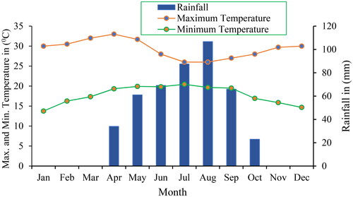
The Vea catchment is located between latitudes 10° 30′ and 11° 08′ N and longitudes 1° 15′W and 0° 50′E (Figure 1). The catchment mainly covers Bongo and Bolgatanga districts in Ghana and south-central Burkina Faso (Larbi et al. 2019). The catchment area consists of three agroecological zones in the semi-arid zone with an average yearly rainfall of about 956 mm, and its peak is in August; the basin has a unimodal rainfall regime from May to October (Larbi et al. 2019). The temperature is generally higher than the average annual temperature of 28.9 °C, except for the wet months of July, August, and September. The rainfall and temperature pattern are shown in Figure 2. Potential evaporation exceeds yearly precipitation. The Vea catchment has a relatively low topography with elevations between 89 to 317 meters above sea level. LULC is mainly cropland, followed by grassland with mixed vegetation/forest. The primary economic activity of the inhabitants of this area is agricultural production (Larbi et al. 2019).

Figure 1. Map of the study area with the heterogeneous landscape.

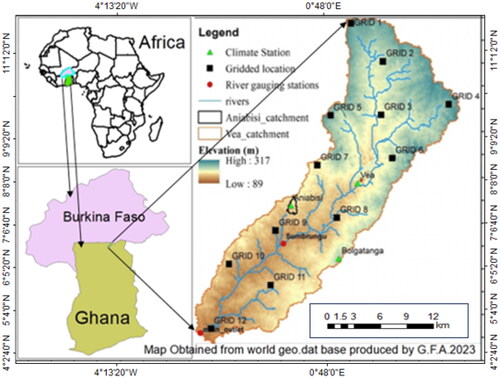
Figure 2. Monthly temperature and rainfall of Vea catchment.

2.2. Data source

2.2.1. Satellite data Sources and methods of acquisition

Satellite images were obtained from the United States Geological Survey (USGS) Data Portal (http://earthexplorer.usgs.gov). World Reference System ‘WRS’, Path 194, Row 52, was applied to select the area of interest. To examine land cover changes in the Vea catchment, four (4) Landsat scenes were captured between 1998 and 2022, each taken eight years apart. Images were taken in November with at least 5% cloud cover to reduce seasonal variation in vegetation and pattern variation. Google Earth Pro was used to reference and validate satellite images. A DEM (Digital Elevation Model) with a resolution of 30 m was obtained from the SRTM (Shuttle Radar Topography Mission) and was also used to collect spatial data. All data (images) are projected to the Universal Transverse Mercator (UTM) Zone 30 N projection system and the World Geodetic System-84 (WGS84) reference to ensure consistency between data sets during analysis. Data collection and other information for each Landsat scene are presented in Table 1.

Table 1. Sources and description of satellite data.

Sensor type	Date of acquisition	Cloud Cover (%)	Pixel resolution	WRS		Spectral resolution
				Path	Row		Bands/colour
Landsat TM	06/11/1998	5	30 × 30	194	52/53	8	Multi-spectral
Landsat7 ETM+	09/11/2006	5	30 × 30	194	52/53	8	Multi-spectral
Landsat 8 (OLI)	23/05/2014	4	30 × 30	194	52/53	11	Multi-spectral
Landsat 8 (OLI)	16/05/2022	4	30 × 30	194	52/53	11	Multi-spectral

OLI: Operational Land Imager; ETM+: Enhanced thematic mapper, Thematic Mapper (TM).

Each Landsat scene’s acquisition dates and further details are displayed in Tables 1 and 2.

Table 2. Description of LULC classes (Larbi et al. 2019).

LULC categories	Description
Cropland	Areas used for crop cultivation
Grassland	The land mostly covered with grasses
Forest	Land covered with dense trees, mixed forests, and plantation forests.
Waterbody	Areas covered with standing or moving water
Built-up area	Areas of human settlements, roads, artificial surfaces, and bare soil

2.2.2. Land use and land cover change assessment

2.2.2.1. Image pre-processing

Environmental resource data analysis system (ERDAS) Imagine version 2015 software is used for preprocessing operations (Arfasa et al. 2023). The most common image preprocessing methods are geometric and radiometric corrections that improve the quality of remotely sensed images for further analysis. Therefore, as suggested by (Arfasa et al. 2023), all images for this study were geometrically corrected and rectified at level 1 (L1T). To reduce errors in the digital number of images and improve their interpretation, radiometric correction is applied (Gong and Luo 2023). The image processing chain was also performed using the open-source software Quantum GIS (QGIS version 3.10) (QGIS, https://qgis.org/en/site/). Atmospheric correction was applied using a semi-automatic classification plugin(Mohajane et al. 2018). was done based on the Dark Object Downloading (DOS) algorithm (Abdurahman et al. 2023). In this study, radiometric correction was applied to the TM, ETM + and OLI images for the years 1998, 2006, 2014 and 2022. The conversion process was performed for each of the TM, ETM + and OLI items at a resolution of 30 m. 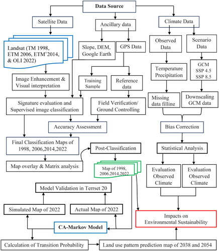For all images, calibration was obtained by converting raw digital numbers (DN) to sensor spectral radiance using Equation (1)(1) $$L\mathrm{\lambda }=(L\mathrm{\lambda }\max -\text{Lλmin})/(\text{QCALλmax}-\text{QCALλmin})\mathrm{x}(\mathrm{DN}-\text{QCALλmin})+\text{Lλmin}$$(1) . A flowchart with the methodology followed in this study is presented in Figure 3. All bands of TM, ETM + and Operational Land Imager (OLI) were considered for layers stacking. After stacking the satellite, data/images were clipped to a subset of the case study area which is 306 km² in order to focus on the relevant data. (1) $$L\mathrm{\lambda }=(L\mathrm{\lambda }\max -\text{Lλmin})/(\text{QCALλmax}-\text{QCALλmin})\mathrm{x}(\mathrm{DN}-\text{QCALλmin})+\text{Lλmin}$$(1)

Where Lλ is the spectral radiance at the sensor’s aperture in mW/(cm²·sr·µm); DN is the digital number of the quantized calibrated pixel value; Lλmax is the maximum spectral radiance that is scaled to QCALλmax; Lλmin is the minimum spectral radiance that is scaled to QCALλmin; QCALλmax is the maximum quantized calibrated pixel value in DN (corresponding to Lλmax); and QCALλmin is the minimum quantized calibrated pixel value in DN (corresponding to Lλmin). After this conversion, the radiance is converted into top-of-atmosphere (TOA) reflectance using Equation (2)(2) $$P=\frac{\pi L{d}^2}{\mathit{ESun}\text{λcosθ}}$$(2) : (2) $$P=\frac{\pi L{d}^2}{\mathit{ESun}\text{λcosθ}}$$(2)

Where q ¼ Unitless planetary reflectance, L ¼ Spectral radiance at sensor aperture, d ¼ the Earth-Sun distance which is on the date of imaging, ESun ¼ Mean solar exoatmospheric irradiance, $\pi =$ Mathematical constant equal to ∼3.14159 [unitless], $\mathrm{\theta }\mathrm{s}=$ Solar zenith angle [degrees].

Figure 3. Comprehensive flowchart land use land cover change and climate change modeling.

2.2.2.2. Image classification

To classify LULC categories, training sites were randomized and used to locate training pixels for each LULC classes. Training sites supported high-resolution images from Google Earth for current imagery generated by GPS readings. For old historical images, Training sites were assigned using visual image interpretation, information from local elders, and local knowledge from researchers. At the evaluation stage, signature editions are made by deleting, merging or renaming until the most satisfactory results are achieved (Ullah et al. 2022). Five LULC classes were identified for image classification based on visual and digital satellite image interpretation and from field verification. Satellite images of 1998, 2006, 2014 and 2022 were used for change detection within 1998–2006, 2006–2014, 2014–2022, and 1998–2022 which were analyzed using ERDAS Imagine 15 upon the application of Support Vector Machine (SVM) classifier algorithm. Because, Support Vector Machines (SVM) is a machine learning algorithm used for classification and regression analysis. SVM is a supervised learning algorithm that works by finding the best hyperplane that separates the data into different classes (Govender et al. 2022; Nageswaran et al. 2022; Abdurahman et al. 2023). SVM is implemented to map various land cover types from a remote sensor image covering an urban area, demonstrating the robustness of this type of pattern recognition technique for mapping heterogeneous landscapes. In terms of classification accuracy, SVM can perform better than maximum likelihood (MLC) or decision tree (DC), and multilayer perceptron neural networks (MLP). The SVM is a method that is widely recommended in literatures for its capability to accurately classify diverse LULC types, particularly in data-scarce areas. SVM is a supervised classification method derived from statistical learning theory (Thakur and Manekar 2022). Support vector machine is well-suited to handle complex spectral classes as they fit a separating linear hyperplane between classes in the multidimensional feature space. Image enhancement and composition will be applied to better discriminate the LULC classes. In accuracy assessment overall accuracy, kappa coefficient, the producer’s accuracy (accounting for errors of omission), and user accuracy (accounting for errors of commission) were used to verify the classification using confusion matrix (error matrix) application in ERDAS software (Abdurahman et al. 2023; Nath et al. 2023).

2.2.2.3. Accuracy assessment

Accuracy assessment tells us to what extent the ground truth is depicted on the equivalent classified image (Abbas and Jaber 2020). The classification accuracy assessment provides the degree of reliability of the results and subsequent change detection (Brown et al. 2020). The error matrix is the most used technique for determining accuracy (Shao et al. 2019). The classification accuracy can be evaluated to produce an overall measure of the map’s quality, which can then be used to compare alternative change detection systems. The minimum level of accuracy in interpreting remote sensing data to identify LULC classes should be at least 85% (Aljenaid et al. 2022). These standards error matrices are computed based on the same data references for each image to calculate the components of overall accuracy, user’s accuracy, producer’s accuracy, error of commission (EC), error of omission (EO), and kappa coefficient.

Overall accuracy (OA) is the total number of successes compared to the total number of samples in the categorized image. It is calculated by summing the number of correctly classified values and dividing it by the total number of values in the confusion matrix in Equation (3)(3) $$OA=\frac{\text{Sum of diagonal tallied }\left(\text{correctly indentified}\right)}{\text{Total number of samples}}\mathrm{*}1003$$(3) . User’s accuracy (UA) is the probability of classified pixel on each map representing the actual class on the ground or real-world location and is calculated using Equation (4)(7) $$\mathrm{KC}= \frac{\mathrm{N}\sum \text{r i}=1\text{xii }\text{-}\mathrm{ }\sum \text{r i}=1\mathrm{ }(\mathrm{xi}+\mathrm{ }\times \mathrm{ }\mathrm{x}+1)}{\mathrm{N}2\mathrm{ }\text{-}\mathrm{ }\sum \text{r i}=1(\mathrm{xi}+\mathrm{ }\times \mathrm{ }\mathrm{x}+1)\mathrm{ }}\mathrm{*}100$$(7) . On the other hand, the producer’s accuracy (PA) measures the error of omission. It is the probability that a reference pixel is classified correctly. It is calculated by dividing the number of corrected classified samples of a specific category by the total number of reference samples using Equation (5)(8) $$MC\left({km}^2\right)=Af-Ai$$(8) . The error of commission (EC) is the proportion of a pixel that is predicted to be in a class, but it does not. It is calculated using Equation (6)(9) $$PC\left(\%\right)=\frac{Af-Ai}{Ai}*100$$(9) . The error of omission (EO) is the proportion of observed pixels on the ground that are not classified on the map, and it corresponds to the producer’s accuracy. The kappa coefficient (KC) is a measure of the difference between the actual agreement between reference data and an automated classifier and the chance agreement between the reference data and a random classifier, expressed using Equation (7)(7) $$\mathrm{KC}= \frac{\mathrm{N}\sum \text{r i}=1\text{xii }\text{-}\mathrm{ }\sum \text{r i}=1\mathrm{ }(\mathrm{xi}+\mathrm{ }\times \mathrm{ }\mathrm{x}+1)}{\mathrm{N}2\mathrm{ }\text{-}\mathrm{ }\sum \text{r i}=1(\mathrm{xi}+\mathrm{ }\times \mathrm{ }\mathrm{x}+1)\mathrm{ }}\mathrm{*}100$$(7) . The percentage of correctly categorized pixels is calculated from the percentage expected by chance. It measures the difference between the actual agreement and chance (random) agreement between the map and the validation data on the ground (Visa et al. 2011). The higher the classification accuracy of the map, the more valuable it is for land administrators and land-use planners. The KC (Rwanga and Ndambuki 2017) is a discrete multivariate approach for determining the level of agreement or accuracy. Its value ranges from −1 to 1. However, it frequently falls between 0 and 1 (Foody 2020).

Overall Accuracy (OA) (3) $$OA=\frac{\text{Sum of diagonal tallied }\left(\text{correctly indentified}\right)}{\text{Total number of samples}}\mathrm{*}1003$$(3)

Users Accuracy (UA) (4) $$UA=\frac{\text{Samples correctly identified in the row}}{\text{Row total}}*100$$(4)

Producer’s Accuracy (PA) (5) $$PA=\frac{\text{Samples correctly identified in the column}}{\text{Column total }}*100$$(5)

Error of Omission (EO) (6) $$EO=\frac{\sum \text{ of f Diagonal element of Column}}{\text{Column Total}}*100$$(6)

Kappa Coefficient (KC) (7) $$\mathrm{KC}= \frac{\mathrm{N}\sum \text{r i}=1\text{xii }\text{-}\mathrm{ }\sum \text{r i}=1\mathrm{ }(\mathrm{xi}+\mathrm{ }\times \mathrm{ }\mathrm{x}+1)}{\mathrm{N}2\mathrm{ }\text{-}\mathrm{ }\sum \text{r i}=1(\mathrm{xi}+\mathrm{ }\times \mathrm{ }\mathrm{x}+1)\mathrm{ }}\mathrm{*}100$$(7) where r is the rows number in the matrix, xii is the number of observations in row i and column i (the diagonal elements), x + i and xi + are the marginal totals of row i and column j, respectively, and N is the observations’ number.

2.2.2.4. Change detection

Due to the availability of large storage data sets, a number of numerical change detection algorithms and methods have been developed and studied over the past decades to estimate and detect LULC changes (Lu et al. 2014). These methods and procedures have been thoroughly reviewed, with excellent descriptions and summaries provided. The most common approaches for change detection include image contrast, image segmentation, PCA, CVA, and post-classification comparison (Hansen 2022). Recently, there has been much debate about the application of machine learning algorithms to remote sensing images (Maxwell et al. 2018). In this study, we investigated and detected changes in the spatial extent and model of the study area through a change detection method based on QGIS, which combines GIS and ERDAS images. For each type of LULC, the area in km² and the percentage change for the periods 1998–2006, 2006–2014, 2014–2022 and 1998–2022 were calculated to analyze land cover change in the study area. Although the LULC statistics are calculated differently, the change in LULC over the four time periods is based on the difference between the years 1998, 2006, 2014 and 2022. Magnitude of Change (MC), Percentage change (PC) and rate of change (ARC) of the classified images were calculated based on the following equations: (8) $$MC\left({km}^2\right)=Af-Ai$$(8) (9) $$PC\left(\%\right)=\frac{Af-Ai}{Ai}*100$$(9) (10) $$\mathit{ARC}\left({km}^2{\mathit{year}}^{-1}\right)=\frac{Af-Ai}{n}$$(10) (11) $$\left(\text{Rate of change}\left(\mathrm{R}\right)\left(\frac{\mathrm{ha}}{\mathrm{yr}}\right)=\frac{\text{Area final year}-\text{Area initial year}}{\text{area initial year}}\times 1/\left(\text{time interval}\right)\times 100)\right)$$(11)

Where Ai is the class area (km²) at the initial time, Af is the class area (km²) at the final time, and (n) is the number of years of the study period.

Loss = Row total - diagonals of each class

Gain = column total – diagonals of each class

Net change = gain-loss

Net persistence = Net change/diagonals of each class

2.2.2.5. Annual rate of change analysis

The difference between the final year and the initial year, determining the magnitude of change between corresponding years, will be divided by the initial year and period to obtain the annual rate of change for each land use type. For determining the spatiotemporal size and rate of change in LULC categories (Equation (12))(12) $$\mathrm{ARC}\left(\%\right)=\frac{\mathrm{Fy}\text{-}\mathrm{Iy}}{\text{Iy*t}}*100$$(12) : (12) $$\mathrm{ARC}\left(\%\right)=\frac{\mathrm{Fy}\text{-}\mathrm{Iy}}{\text{Iy*t}}*100$$(12)

Where ARC is the annual rate of change in LULC categories. Iy and Fy are the initial and final year areas, respectively, and t is the time interval.

2.2.3. Simulation and prediction of land use/cover changes

2.2.3.1. Markov-chain model analysis

The Markov chain model is a unique and widely used land use and land cover modeling tool that represents LULCC as a stochastic process. In a Markov system, the future state of the crop system is modeled based on the immediate state of progress. The transition of the system from one state to another is a transition, and the probability associated with that state transition is called the transition probability. The initial estimates of $\mathit{pij}$ can be computed as (13) $${\mathit{P}}_{\mathit{ij}}={\mathit{P}}_{\mathit{ij}}/{\mathit{N}}_{\mathit{t}}(\mathit{ij}\dots 1,2,3,\dots .\mathit{m})$$(13)

Where $\mathit{Nij}$ is the number of units transitioned from the state i to state j, $\mathit{Ni}$ is the number of units in state i.

Therefore, the basic hypothesis of the Model simulation process mainly produces a Land Use area transfer matrix and a probability transfer matrix to predict land use change. The Markov Chain Model is described as a set of states, S = (S_1, S_2, S_3,…S_n) assuming that the current state is〖 S〗_t and then, it changes to state S_j at the next step with a probability denoted by transition probabilities P_IJ Thus, the state S_(t + 1) in the system determined by former stage S_t in the Markov Chain using the following formula (Xiong et al. 2018): (14) $${\mathit{P}}_{\mathit{ij}}=\left[\begin{array}{ccc}{\mathit{P}}_{\mathit{ll}}& \cdots & {\mathit{P}}_{\mathit{ln}}\\ ⋮& \ddots & ⋮\\ {\mathit{P}}_{\mathit{nl}}& \cdots & {\mathit{P}}_{\mathit{nn}}\end{array}\right](0\le {\mathit{P}}_{\mathit{ij}}\le \mathit{l} \mathit{and}\sum \mathit{Pij}=\mathit{li},\mathit{j},\dots ,\mathit{n})$$(14) $${\mathit{S}}_{\mathit{t}+1}={\mathit{P}}_{\mathit{ij} }\times {\mathit{P}}_{\mathit{t}}\dots .$$

Where $P_{ij}$ is the state transition probability matrix and n are the land represents the number of land use type; S is land use status, t; t + 1 is the time point. In this study, Markov chain analysis was conducted in three periods; 1998–2006, 2006–2014, 2014–2022 and 2022–2054. In this way, the matrix of the transition area of ​​land use and the transition probability matrix for the current periods were determined.

2.2.3.2. Cellular automata (CA)

The CA model is a change model with local interaction that reflects the evolution of the system, where space and time are treated as discrete entities, and space is often represented as a regular two-dimensional grid. The temporal and spatial complexity of land use land cover systems can be well modeled by properly specifying transition rules in CA models. CA modeling provides important information for understanding theories of forest cover, such as the evolution of forms and structures. Cellular Automata is a bottom-up dynamic model within a spatio-temporal computation. It is discrete in space-time and the state can perform complex time-space modeling. The data for each cell in the St + 1 state is determined by the cell itself and its neighboring cells in the St state, which means that changes in the cell are handled according to the rules. It mainly consists of cells, cell space, neighbor, rule and time. The CA model filter identifies neighbors (Long et al. 2018). The smaller the distance between the original cell and its neighbor, the greater the weighting factor. The weight factor is combined with the transition probability to predict the state of neighboring network cells. See above that land use changes are not entirely random decisions. In this study, the cellular automata network represented each land use cell, and each network had 8 neighboring cells; Cell status represented the type of land use of the cell; The time interval is 24 years. To track land use transitions, the maximum transition probability rule and the hysteresis rule are valid. If a cell is assigned a land use type, the cell will not change to other land use types during the simulation period (Aburas et al. 2016; Vázquez-Quintero et al. 2016; Gharaibeh et al. 2020). (15) $$\mathrm{St}+1=\mathrm{f}(\mathrm{St},\mathrm{N})$$(15)

Where S is the set of states of the finite cells. t and t + 1 are different moments; N is the neighborhood of cells; and f is the local space transformation rule.

2.3. Climate data source

2.3.1. Historical (observed) climate data source

Historical daily rainfall, maximum and minimum temperature covering the period from 1993 to 2022 for the Vea, and Bolgatanga automatic weather stations within the Vea catchment were obtained from the Ghana Meteorological Agency. Climate data is required to evaluate past and future climate change and the impact environmental sustainability. Due to the sparse distribution of in situ climate stations throughout the catchment, additional daily values of rainfall for 12 gridded sites were extracted from the Climate Hazards Group Infrared Precipitation with Station (CHIRPS) data to complement the in-situ datasets. CHIRPS combines satellite imagery with on-site station data to create gridded time series of rainfall at a resolution of 0.05°. The three agro ecological zones in the study area the north Sudanese Savanna zone (Grid1 and Grid2), Savanna zone (Grid3, Grid4, Grid5, Grid6, Grid7, and Grid 8), and Guinea Savanna zone (Grid9, Grid10, Grid11, and Grid12), were chosen to correspond to these gridded locations. This dataset provided a good representation of real meteorological events and climate trends. The feasibility of the CHIRPS data in reproducing the climatology of the Vea catchment has been examined in a previous study by (Arfasa et al. 2023). The temperature data from the NASA POWER project are extracted from Modern Era Retrospective-Analysis for Research and Applications (MERRA-2) assimilation model products and GEOS 5.12.4 near-real-time products (Arshad et al. 2021). These two satellite products have been selected based on their ability to accurately reproduce the climatology in the Vea catchment within Ghana (Larbi et al. 2021). Data quality control in terms of missing data checks for the two climate stations were performed. Less than 10% missing data records for rainfall and temperature were found for each of the two climate stations.

2.3.2. Global climate models (GCMs) and scenario data source

In this study, Six GCM models from the Coupled Model Inter-comparison project phase six (CMIP6) were used for future climate change projections and assessments under two SSP 4.5 and SSP 8.5 emission scenarios for the Vea catchment. Table 3 shows GCMs models: CanESM5, CNRM-CM6-1, IPSL-CM6A-ATM-HR, MIROC6, MPI-ESM1-2-LR and NorESM2-LM were selected based on previous studies conducted in the Volta basin and Tono basin (Okafor et al. 2017; Larbi et al. 2022). Future time precipitation, and temperature data for the SSP 4.5 and SSP 8.5 emission scenarios will be downloaded using the CMIP6 model from (https://pcmdi.llnl.gov/mips/cmip6/dataportal.html//) node portal of the IPCC database distribution center).

Table 3. Models to download CMIP6 climate data.

No	CMIP6 model name	Country	Horizontal resolution (long. by lat. in degrees)	Variant label
1	CanESM5	Canada	2.8°× 2.8°	r1i1p1f1
2	MPI-ESM1-2-LR	Germany	1.9°× 1.9°	r1i1p1f1
3	IPSL-CM6A	France	2.5°× 1.3°	r1i1p1f1
4	MIROC6	Japan	1.4°× 1.4°	r1i1p1f1
5	CNRM-CM6	Germany	0.9°× 0.9°	r1i1p1f1
6	NorESM2-LM	Norway	2.5°× 1.9°	r1i1p1f1

Source: https://pcmdi.llnl.gov/mips/cmip6/dataportal.html (Gyamfi et al. 2021).

2.3.3. Downscaling GCM data using CMhyd and R programming

Climate projections for the future are typically generated through the use of global climate models (GCMs) (Hewitt et al. 2021). GCMs are scientific tools that replicate the complete climate system of the Earth, encompassing the oceans, atmosphere, and land. They are designed to depict large-scale climate patterns across continents and have been proven to accurately represent general patterns as observed in meteorological datasets from the twentieth century (Manski et al. 2021). These GCMs offer well-configured environments for examining the impact of various future greenhouse gas emissions on the climate of the Earth. The downscaled model output is more realistic than the GCM model output for direct application as hydrological model input and regional-scale assessments for climate change impact (Orkodjo et al. 2022). R software Version 4.6.2. was used for extracting GCM data to the study area and CMhyd was used for downscaling GCM to Specific to the study area. Downscaling from GCMs to RCMs is necessary before using GCM model data as input for the hydrological model (Dessu and Melesse 2013)

2.3.4. Bias correction

Prior to using climatic data for models of climate change and studies on its impacts, biases typically need to be corrected (Hosseinzadehtalaei et al. 2021). Because, GCM model output data usually has a significant bias, which necessitates correlation to analyze data bias reduction, improve data quality, and increase data reliability (Her et al. 2019). Hydrological modeling software (CMhyd) climate model data were utilized in this study to correct bias and remove bias from future climate daily temperature and precipitation data. For this study, we downloaded CMhyd software from https://swat.tamu.edu/software/. The variance scaling bias-correction method was used to correct both the mean and variance of the temperature time series (Fang et al. 2015). The local intensity scaling (LOCI) method of precipitation bias correction in addition to wet-day frequencies and intensities (Smitha et al. 2018). The bias-corrected rainfall and temperature-simulated data (GCM) were used to assess the projected changes in rainfall and temperature at the Vea catchment under the SSP4.5 and SSP8.5 scenarios. The change analysis was conducted for the period 2023–2052 (Near-future), and 2071–2100 (Far-future) relative to the 1993–2022 reference period.

3. Results

3.1. Historical (past) land use/land cover change

3.1.1. Accuracy assessment

The accuracy of LULC change was measured by constructing an error matrix for each classified LULC map from 1998, 2006, 2014, and 2022. producer accuracy, user accuracy, and overall accuracy were used for evaluation. The accuracy measures, including overall accuracy, producer’s accuracy, and user’s accuracy for the classified images during the study periods, showed excellent accuracy in all classes. Table 4 shows the accuracy of classified LULC classes in the Vea catchment over time.

Table 4. Accuracy assessment for 1998, 2006, 2014, and 2022 classified images.

LULC classes	1998		2006		2014		2022
	PA	UA	PA	UA	PA	UA	PA	UA
Built-up/bare land	93.1	90	100	93.3	100	93.3	96.5	93.3
Cropland	93.1	87.1	93.9	91.2	90	97.3	87.2	94.4
Grass land	97.8	96.6	89.5	97.5	97.2	98.6	100	90.4
Mixed v/forest	88.9	97.6	94.6	85.5	94.7	94.7	94.1	100
Water	97	97	95.5	98.4	98.2	94.8	100	93
Overall accuracy	95		93.7		95.9		95.2

The accuracy assessments based on error matrices generated an overall accuracy of 95%, 93.7%, 95.9%, and 93.7% for 1998, 2006, 2014, and 2022. According to Rahmani et al. (2022), the recommended minimum level of accuracy is around 80%, so classified LULC maps are generally acceptable for change analysis. Per the study conducted by (Hudait and Patel 2022). the accuracy of the LULC map is evaluated by constructing an error matrix or confusion matrix, which compares the classified map with a reference classification map. The findings of this study align with the results of other similar studies conducted by (Arfasa et al. 2023) in Ghana, (Chaaban et al. 2022) in Syria, (Abdurahman et al. 2023) in Ethiopia, and (Ntukey et al. 2022) in Tanzania.

3.1.2. Land use/land cover classification

Grasslands and mixed vegetation/forests were not maintained during the study period; therefore, a tendency to decrease their conversion to cropland was observed over time. Therefore, the proportion of land used for cropping increased from 36.1 km² in 1998 to 86.4 km² in 2006 to 120.8 km² in 2014 to 171.5 km² in 2022 (Figure 4).

Figure 4. The LULC of the Vea catchment in 1998, 2006, 2014, and 2022.

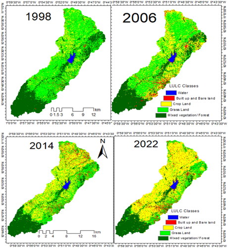
Built-up/bare land increases in tandem with the trend of cropland, and by 2022 the area covered will be about 3.96 times larger than in 1998. The LULC classification results from the Landsat ETM + imagery of 2006 (Table 5) indicates that approximately 1.1% of the area was water, 29.1% was mixed vegetation/forest, 39.7% was grassland, 26.2% was cropland, 4% was built-up area/bare land. These results indicate that LULC in 2006 was dominated by mixed vegetation/forest and grassland areas. According to the Landsat OLI image from 2014 (Figure 4), about 1% of the area was water, 23.6% was mixed vegetation/forestland, 32.6% was grassland, 36.6% was cropland, and 6.3% was built-up area/bare land. These findings show that built-up/bare land and cultivated areas increased in 2014. Water, grassland, and mixed vegetation/forested land show decreasing trends. In addition, the LULC classification results from the Landsat OLI image of 2022 show that about 1% of the land area is water, 22.71% is mixed vegetation/forest land, 18, 14% is grassland, 51.98% is cropland, 6.3% is build-up or bare land. This finding demonstrates that cropland is dominant in the catchment. Generally, grassland decreased, mixed vegetation/forest, and water. However, cropland, built-up area/bare land was observed in the study catchment increased. As Ghana’s population grows and the country strives to achieve food security as part of its poverty reduction strategy, there is a projected increase in agricultural land, resulting in the conversion of forest and grassland into cropland. This conversion process leads to environmental degradation. Concurrently, the water area has decreased per the decline observed in grasslands and forestlands. By 2022, the water area had decreased to a size approximately 0.08 times larger than its extent in 1998 (Table 5).

Table 5. LULC change of Vea catchment from 1998 to 2022.

LULC classes	1998		2006		2014		2022
	km^2	%	km^2	%	km^2	%	km^2	%
Built-up/bare land	5.1	1.6	13.1	4	20.5	6.3	20.2	6.1
Cropland	36.1	10.9	86.4	26.2	120.8	36.6	171.5	51.98
Grass land	181	54.8	131	39.7	107.6	32.6	60	18.14
Mixed v/forest	104.5	31.7	96.2	29.1	77.8	23.6	75.1	22.73
Water	3.5	1.1	3.46	1.1	3.43	1	3.42	1.05

The findings of Atulley et al. (2022) corroborated that the analysis of land cover change in Ghana revealed a consistent expansion of agricultural land and urban built-up areas, accompanied by a decline in savannah forest. Consequently, the curve number increased from 81 in 1986 to 86 in 2040. According to a study conducted in China (Liu et al. 2021), the LULC data showed that between 1980 and 1996, cropland increased while grassland and water decreased. The biodiversity of the Lake Victoria basin in Eastern Africa is adversely affected by land use/land cover change (Katusiime et al. 2023). In the Shashogo district of southern Ethiopia, the cropland increased by 36.2% over 37 years between 1973 and 2005 (Beyamo 2010). According to Wubie et al. (2016), there was a significant change in land cover in the Gumara watershed of the Lake Tana Basin in northwest Ethiopia between 1957 and 2005. During this period, cropland and built-up areas experienced a substantial increase of 21.9%. In contrast, there was a significant decrease in forestland (85.3%), grassland (76.1%), and water (72.54%) within the same timeframe. According to (Naikoo et al. 2020; Atulley et al. 2022), the rate of change in LULC for cropland and built-up was positive between 1991 and 2003. In contrast, due to the concurrently significant increase in farmlands from 18.7% to 47.9%, the Mixed vegetation/forest in the Vea catchment substantially decreased from 29.4% (1985) to 9.9% (2020) (Larbi 2023). Similarly, a study conducted in the Wa East district of Northern Ghana by Basommi et al. (2015), revealed changes in land cover. The open savannah decreased from 50.80% to 36.5%, while the closed savannah decreased from 27.80% to 22.67%. Concurrently, there was an increase in built-up areas within the district.

3.1.3. LULC change detection

The change detection analysis focused on four time periods by constructing four regional matrices from 1998 to 2006, 2006 to 2014, 2014 to 2022, and 1998 to 2022 for 24 years from 1998 to 2022. Table 5 depicts the LULC classes for 1998, 2006, 2014, and 2022, the total area and spatiotemporal changes in the last 24 years, indicating that cropland and built-up/bare land have increased. While grassland, water, and mixed vegetation/forest decreased. A comparison of 1998 and 2006 statistics shows that the grassland, water, and mixed vegetation/forest area decreased by 6.25, 0.005, and 1.04 km². The built-up and cropland areas increased by 1 and 6.28 km², respectively. Between 2006 and 2014, the changes show a 2.9, 0.004, and 2.3 km² decrease in grassland, water, and mixed vegetation/forest areas, respectively. The built-up and cropland areas increased to 0.92 and 4.2 km², respectively. According to changes over the last eight (8) years, cropland is the most dominant category.

From 2014 and 2022, the changes show a 5.95, 0.001, and 0.34 km² decrease in grassland, water, and mixed vegetation/forest areas, respectively. The built-up and cropland areas have increased to 0.04 and 6.34 km², respectively. Cropland appears to be the most dominant category based on changes over the last 24 years. Between 1998 and 2022, the changes show a 15.12, 0.01, and 3.5 km² decrease in grassland, water, and mixed vegetation/forest areas, respectively. The built-up and cropland areas have increased to 1.89 and 16.92 km², respectively. From 1998 to 2022, the built-up area increased from 5.1 km² of the total area of the Vea catchment in 1998 to 20.2 km² in 2022. In addition, cropland increased from 36.1 km² in 1998 to 171.5 km² of the total area in 2022. Grasslands, water, and mixed vegetation/forest have all lost 121 km², 0.08, and 29.4 km² of land, respectively. The generated change maps and matrices were employed to comprehend how the status and magnitude rate changed over the years. The three LULC classes show negative annual changes between 1998 and 2022. Annual losses in the grassland, water, and mixed vegetation/forest classes were −0.15 km², −0.01 km², and −3.67 km², respectively. For the same period, these classes’ annual rate of change (ARC) was −8.35%, −2.58%, and −3.5%, respectively.

3.1.3.1. LULC change detection from 1998 to 2022

Between 1998 and 2022, grassland, water, and mixed vegetation/forest were negative. Most areas were mostly converted to cropland 146.87 km² and built-up area/bare land 14.45 km². During this period, the mixed vegetation/forest class lost 29.9 km² and was mostly converted to cropland and built-up/bare land. In addition, the grassland class lost 151.5 km² in 2022, converted to cropland, mixed vegetation/forest, and built-up/bare land. In 2022, 137.7 km² of grasslands were converted to cropland, and 12.4 km² in 2022 were converted to built-up areas/bare land.

Furthermore, 0.03 km² of water in 2022 was converted to built-up areas, grassland, and cropland in 2022. Approximately 0.26 km² of the built-up area in 2022 was lost to grassland areas. Bolded transitions in Table 6 show how from 1998 to 2022, LULC classes changed. The prominent classes in 2022 were cropland. In 2022, the grassland area decreased by more than 25.19 km². The change detection from 1998 to 2022 indicates a shift to cropland and built-up spaces and a decrease in grassland, water, and mixed vegetation/forest. However, cropland is the dominant class in the Vea catchment. The research also noted a comparable finding to Larbi et al. (2019), which discovered a decline in forest and dense woodland regions alongside a rise in human settlements and cultivated land (from 46.5% to 49.2%) between 1990 and 2015. This observation was made using a multidimensional methodology to evaluate land degradation in the Nawuni area, a sub-basin located within the White Volta basin.

Table 6. Land use the land cover transition of the Vea catchment from (1998–2022).

LULC classes		2022
		Built up	Cropland	Grassland	Forest	Water	Row total	Loss
1998	Built-up/bare land	3.85	0.15	0.26	0.00	0.00	4.3	0.4
	Cropland	0.26	27.79	5.66	0.01	0.00	33.7	5.9
	Grassland	12.40	137.7	33.81	1.43	0.00	185.4	151.5
	Mixed V./Forest	1.69	8.99	19.27	73.33	0.00	103.3	29.9
	Water	0.03	0.026	0.03	0.00	3.42	3.5	0.08
	Column total	18.3	174.66	59.0	74.78	3.42	–	–
	Gain	14.45	146.87	25.19	1.45	0	–	–
	Net change	14.01	140.94	−126.37	−28.5	0	–	–
	Net persistence	3.64	5.07	−3.83	−0.39	0	–	–

Note: Those figures in bold are the sum of diagonals and represent overall persistence.

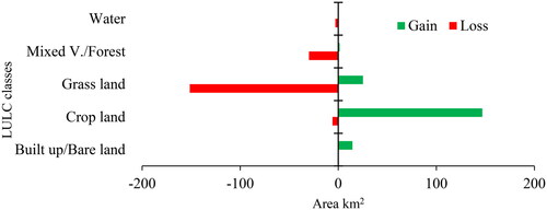
Figure 5 shows the gain and losses of land use classes. Between 1998 and 2022, grassland, mixed vegetation/forest lost their area, while cropland and Built-up/bare land gained. Grass land lost huge area, in contrast cropland gained huge area

Figure 5. Gains and losses of LULC classes from 1998 to 2022.

3.2. Future land use/land cover change

3.2.1. Model validation

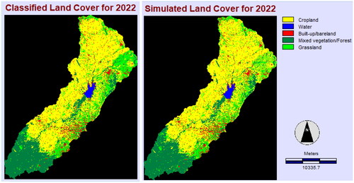
Comparisons between actual and simulated LULC 2022 maps were performed to validate the predicted maps. The validation results between the simulated and actual LULC test summary of the model are presented in Table 7. The accuracy of the prediction was confirmed by comparing the predicted LULC for 2022 with the classified LULC for the same year. The statistics show that K_no is 0.9016, K_location is 0.9120, and K-standard, which is the overall kappa, is 0.9043. This means that the simulation is perfectly capable of pinpointing the location and also the quantity. Therefore, there is very little quantification and location error and all K-index values ​​exceed the minimum acceptable standard of 82% (Arfasa et al. 2023). In this study all values of Kappa indices are greater than 95%, meaning that the agreement between the predicted and the actual map of 2022 is relatively high, showing a strong projection ability of the model to utilize it for LULC change pre-diction in 2038 and 2054 (Table 8). LULC prediction of the landscape of the current study is based on the change of driver effects.

Table 7. Actual and simulated LULC changes in area in 2022.

LULC classes	Actual area		Simulated area		Net area difference (%)
	km2	%	km2	%
Cropland	174.5	52.87	176.2	53.4	0.50
Water	3.41	1.03	3.4	1.03	0.00
Built-up/bare land	22.3	6.75	22.6	6.84	0.09
Mixed v/Forest	75.16	22.7	74.5	22.6	−0.01
Grassland	54.9	16.6	53.5	16.2	−0.4

Table 8. The k-index values of the simulated LULC map of 2022.

Index	Value
K no	0.9016
K Location	0.9120
K standard	0.9043

The visual comparison between the actual LULC 2022 map and the simulated map (Figure 6) is relatively similar. The common area of ​​all land use types from the actual and simulated maps also shows an acceptable decision range, where the difference in actual area between the simulated map and the 2022 reality for all LULC types is less than 5% (Table 7). Regardless of the magnitude of variability among the classified land-use types, the best agreement of change trends was observed with past LULC changes and predicted LULC change outcomes. The high degree of consistency between the actual and predicted spatial land use distribution confirms that the developed CA-Markov model is best suited for predicting changes in the LULC of the Vea catchment in 2038 and 2054.

Figure 6. Simulated and actual LULC maps of 2022.

3.2.2. Prediction of LULC changes

The predicted land use/land cover types for 2038 and 2054 were calculated using the CA Markov model and are plotted in areal in Table 9. The area of ​​grassland and mixed vegetation/forest decreased from 54.9 km² in 2022 to 52 km² in 2038 and 72 km² in 2022 to 72 km² in 2054. From 2038 (179 km²) to 2054 (182 km²) and from 2038 (24 km²) to 2054 (25.2 km²) there will be a continuous increase in cropland and built-up/bare land. On the other hand, the amount of water will decrease from 2038 (3.1 km²) to 2054 (3 km²). The expansion of cropland and built-up/bare land is expected to increase at the expense of mixed vegetation/forest and grassland. Over 2022–2054 grassland and mixed v./forest would have exhibited the highest loss by 4.9 km², and 5.2 ha respectively (Table 9). The lowest loss could be scored by water body. While the highest gain would be observed in cropland (Figure 7).

Table 9. LULC area coverage, and rate of changes between 2022 and 2054.

LULC classes	Area of 2022		Area of 2038		Area of 2054		Gain/loss 2022–2054 (%)
	km^2	%	km^2	%	km^2	%	km^2	%	Annual change (%)
Cropland	174.5	52.87	179	54.24	182	55.15	7.5	4.3	0.13
Water	3.41	1.03	3.1	0.94	3	0.91	−0.41	−12	−0.37
Built-up/bare land	22.3	6.75	24	7.3	25.2	7.64	2.9	13.01	0.45
Mixed v/Forest	75.2	22.7	72	21.8	70	21.2	−5.2	−7.1	−0.22
Grassland	54.9	16.6	52.1	15.8	50	15.2	−4.9	−8.9	−0.31

3.3. Historical (past) and future climate change

3.3.1. Evaluation of Historical annual temperature

The findings of the trend test showed statistically significant positive increasing baseline annual and seasonal maximum and minimum temperature trends. The findings revealed a noteworthy positive increase trend at two meteorological gauging stations and eight grid stations. However, two meteorological grid stations displayed a significant negative decrease trend, and two grid stations showed no significant overall change in temperature, as presented (Figure 8).

3.3.2. Evaluation of projected annual temperature

The analysis of yearly and seasonal temperature variations revealed significant temperature trends in the 60-year periods of 2023–2052 and 2071–2100. The projected minimum and maximum temperatures in the catchment area were determined using the SSP 8.5 and SSP 4.5 emission scenarios for two future time periods: the near-future (2023–2052) and the far-future (2071–2100). The analysis of trends showed that both the SSP 8.5 and SSP 4.5 scenarios predicted a notable increase in the annual average temperature. The results of the trend test analysis are shown in (Figures 9 and 10), which show that the annual minimum and maximum temperatures in the catchment area show increasing trends for the two (2) time periods under the SSP 4.5 and SSP 8.5 emission scenario.

3.3.3. Evaluation of observed annual precipitation

Trends between 1993 and 2022 were statistically significant, according to a 30-year analysis of annual and seasonal variations in precipitation. For the baseline period of change in precipitation trend for the Vea catchment. Two (2) precipitation measurement stations and 12 Gridded stations from CHRIPS data were examined. For the nine (9) grid stations and two (2) meteorological measuring stations within the basin analysis of the annual precipitation data trends of the time series showed seasonal variation trends. None of the three (3) grid weather stations in (Figure 11) displayed monotonic trend changes in annual precipitation that were statistically significant, according to the trend detection test.

3.3.4. Evaluation of projected annual precipitation

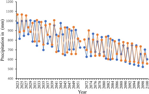
Statistically significant trends for the years (2023–2052 and 2071–2100) over 60 years were discovered after evaluating the change in precipitation on an annual and seasonal basis. Based on the results of the trend tests for the SSP 4.5 and SSP 8.5 emission scenarios, a significant decrease in annual precipitation amounts was predicted. The predicted precipitation for the Vea catchment was assessed for two (2) future periods: the near term (2023–2052), and the long term (2071–2100) when compared to the reference time (Figure 12).

4. Discussion

4.1. Past and future land use/land cover change

The Vea catchment LULC classes have been identified based on typical land covers, the variety of reflectance of characteristics of images from Landsat, detailed primary data, and a review of related literature. Cropland, grassland, and mixed vegetation were the prominent land cover classes, while water and built-up/bare land were less dominant from 1998 to 2022. From the total area, cropland shows an increasing trend which covered an area in km² or (%) of about 36.1 km² (10.9%) in 1998 to 171.5 km² (51.98%) in 2022, and built-up/bare land also increased from 5.1 km² (1.6%) in 1998 to 20.2 km² (6.1%) in 2022. This result is supported by earlier studies conducted in several regions of Ghana (Appiah et al. 2015; Agariga et al. 2021; Gbedzi et al. 2022; Baidoo et al. 2023; Larbi 2023). For instance, this study concluded that cropland constituted the most LULC type in the Vea catchment from 1998 to 2022. The LULC map classification accuracy assessment in 1998, 2006, 2014, and 2022 showed an excellent outcome. The accuracy of 1998, 2006, 2014, and 2022 LULC maps were 95%, 93.7%, 95.9%, and 93.7%, respectively. The findings from this study show that the ground truth LULC classes and classified maps confirmed that the classified maps agreed with the minimum accuracy required for the next post-classification techniques (Agariga et al. 2021). The findings revealed that LULC has changed in the Vea catchment over the last 24 years (1998–2022). Cropland and built-up/bare land have grown significantly in the study catchment, increasing by 51.98% and 6.1% between 1998–2022. In contrast, for this period, grassland, mixed vegetation/forest, and water have decreased by 36.66%, 22.73%, and 1.05%, respectively (Table 5). The results of earlier research were also credible. For instance, Larbi (2023) stated that the loss of grassland and forest from 1986 to 2020 in the Tono basin increased farmland. Issahaku (2023) concluded that agricultural and built-up areas had expanded over the two decades between 1985 and 2016, while grassland, water, and forests decreased.

Comparisons between actual and simulated LULC 2022 maps were performed to validate the predicted maps. The accuracy of the prediction was confirmed by comparing the predicted LULC for 2022 with the classified LULC for the same year. The statistics show that K_no is 0.9016, K_location is 0.9120, and K-standard, which is the overall kappa, is 0.9043. This means that the simulation is perfectly capable of pinpointing the location and also the quantity. Therefore, there is very little quantification and location error and all K-index values ​​exceed the minimum acceptable standard of 82% (Mishra et al. 2019). In this study all values of Kappa indices are greater than 95%, meaning that the agreement between the predicted and the actual map of 2022 is relatively high, showing a strong projection ability of the model to utilize it for LULC change pre-diction in 2038 and 2054 (Table 9).

The predicted land use/land cover types for 2038 and 2054 were calculated using the CA Markov model and are plotted in areal in Table 9. The area of ​​grassland and mixed vegetation/forest decreased from 54.9 km² in 2022 to 52 km² in 2038 and 72 km² in 2022 to 72 km² in 2054. From 2038 (179 km²) to 2054 (182 km²) and from 2038 (24 km²) to 2054 (25.2 km²) there will be a continuous increase in cropland and built-up/bare land. On the other hand, the amount of water will decrease from 2038 (3.1 km²) to 2054 (3 km²). The expansion of cropland and built-up/bare land is expected to increase at the expense of mixed vegetation/forest and grassland. Over 2022–2054 grassland and mixed v./forest would have exhibited the highest loss by 4.9 km², and 5.2 ha respectively (Table 9). The lowest loss could be scored by water body. While the highest gain would be observed in cropland. Planting of maize, millet, sorghum, rice, soya beans, Bambara beans, groundnuts, and pepper is the main source of employment in the catchment, employing over 70% of the working force (Mensah and Fosu-Mensah 2020). The intense farming activities confirm the reasons why cropland increased over the period in the catchment. The residents also use fuel wood as their prime energy source while fetching wood from the forest for housing construction. These activities have collectively contributed to degrading the forest resources in the catchment and negatively affecting environmental sustainability. Studies by identified how unsustainable farming systems and increased cropland enhances CO2 emissions and global warming.

4.2. Past and future climate change

The results of both individual and average GCM climate models indicate that the minimum and maximum temperatures in the Vea catchment should increase between 2023–2052 and 2071–2100. Both climate scenarios confirm this. Under the SSP4.5 and SSP8.5 climate change scenarios, the anticipated minimum and maximum temperature increases were evaluated and compared (Figure 7) with the reference period. According to projections, annual maximum and minimum temperatures will increase by 34 °C, and 28.45 °C under SSP 4.5, while SSP 8.5 will cause an increase of 36 °C, and 29.5 °C throughout future periods, as shown in (Figures 9 and 10) for the future near future (2023–2052), and far future (2071–2100). The average monthly temperature is predicted to increase by 34 °C and 26.45 °C under SSP 4.5 and 34 °C and 27.5 °C according to SSP 8.5, respectively, in the years 2023–2052 and 2071–2100. The results are expected to show that over the study periods, the average temperature will increase from 2.10 to 3.5 °C in the SSP 4.5 and from 2.4 to 4.15° C in SSP 8.5.

Figure 7. The predicted 2038 and 2054 LULC change.

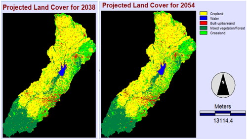
Figure 8. Annual average temperature changes in Vea catchment during (1993–2022).

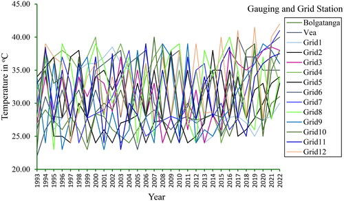
Figure 9. Projected change in annual minimum temperature under SSP4.5 and SSP8.5 emission scenarios (2023–2052, and 2071–2100).

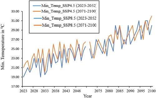
Figure 10. Projected change in annual maximum temperature under SSP4.5 and SSP8.5 emission scenarios (2023–2052, and 2071–2100).

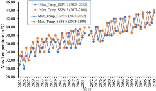
Figure 11. Annual precipitation in (mm) in Vea catchment during (1993–2022).

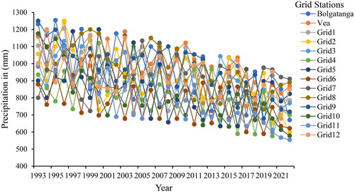
Figure 12. Projected changes in annual precipitation under SSP 4.5 and SSP 8.5 emissions scenarios (2023–2052, and 2071–2100).

The Vea catchment experiences change in temperature, with a range of 1.6 to 2.8 °C under SSP4.5, and a range of 2.1 to 3.4 °C under SSP8.5. According to studies by Sun et al. (2023), the change in temperature between 2.04 and 4.15 °C by the end of the 2100th century would be nearly identical in direction and time in the SSP 4.5 emission scenarios. The results of other studies have been confirmed by the results of this study. According to Çaktu (2022), the future temperature rise is predicted to be between 2.8 and 5 °C. (Ahmed et al. 2015); Amin et al. (2023); (Fotso‐Nguemo et al. 2023) conducted additional studies focusing on West Africa and predicted future temperature increases. In general, the average temperature changes in the Vea catchment range from 2.1 to 3.5 °C under the SSP 4.5 emission scenarios. However, under the SSP 8.5 emission scenarios, the range is from 2.4 to 4.15 °C by the end of the 2100 century. The anticipated rise in temperature will have an impact on the environmental sustainability (Dash and Maity 2023; Sheikh et al. 2023). The environment experiences several negative effects due to high temperatures. These include reduced moisture in the soil, a rise in the frequency of hot days and a decline in cold days annually, greater evapotranspiration, and limited water accessibility. The amount of water that is accessible will be impacted by changes in precipitation, increasing temperatures, and temperature variations. This is due in part to the expectation that increased temperatures will accelerate the evaporation process. The Vea catchment is expected to face increased water stress and higher temperatures in the coming years.

The average annual precipitation of the Vea catchment was estimated to be 800 mm and the annual total was 9600 mm in the most recent count of the reference period (1993–2022). On the other hand, future times of the annual total and average precipitation of the catchment are quantified and projected over the near future (2023–2052), and the far future (2071–2100). The projected annual total and average precipitation would be 10,832 and 361 mm, and 9689, and 322.96 mm under the SSP 4.5 and SSP 8.5 emission scenarios, respectively. According to the SSP4.5 and SSP8.5 emission scenarios, the projected impacts of climate change on future environmental sustainability will be severe. In the near future (2023–2052), and the far future (2071–2100), it is projected that annual precipitation will decrease by 10.01%, and 12.02% under the SSP 4.5 emission scenarios and by 11.05%, and 13.04% under the SSP 8.5 emission scenarios, respectively (Figure 10). As compared to the SSP 8.5 emission scenario, the projected decrease in precipitation under the SSP 4.5 climate change is less. The findings indicate that the Vea catchment precipitation decreased more noticeably under the SSP8.5 scenario than under SSP4.5. In comparison to the SSP 8.5 emission scenarios, the projected decreases in mean annual precipitation for the SSP 4.5 emission scenarios range from 12.34 to 13.10%. Precipitation decreases were projected to be unidirectional under the SSP 4.5 and SSP 8.5 emission scenarios. The findings of this study are consistent with previous studies’ forecasts of future precipitation declines (Adusu et al. 2023; Agodzo et al. 2023; Capps Herron et al. 2023). The results of this study, which are in agreement with previous studies show that precipitation, or the amount of seasonal precipitation decreases as a result of climate change in the Vea catchment (Larbi et al. 2020). As a result, the decrease in precipitation and rise in temperature during the study period will have an impact on the environmental sustainability in the Vea catchment. The results of this study revealed statistically significant relationships between temperature and precipitation environmental sustainability.

4.3. Impacts of land use/land cover, and climate change on environmental sustainability

Human development can negatively impact the natural environment as advances in science and technologies cause environmental harm. Environmental sustainability focuses on sustainability within the natural environment (Tóthová and Heglasová 2022). This includes conserving the natural environment as a whole, including resources within nature such as clean air and clean water, as well as wildlife, for future generations. Land use and land cover and climate changes is central to the sustainability debate (Roy et al. 2022). It has serious ecological repercussions and pose a great deal of challenge to environmental sustainability at local and global scales. Since the Stockholm Conference in 1972 the need for managing environmental resources has become a political agenda in most developed countries of the world. The awareness was raised to its peak at the Rio Earth Summit in 1992 by the global action programme on sustainability – Agenda 21 (Conca and Dabelko 2019). Land use/cover and climate change is the most common type caused by human-induced activities. These phenomena cause biodiversity loss and alteration of essential natural resources (Teck et al. 2023). In Ghana, particularly in Vea catchment, population growth increased current pressure to convert land from natural and agricultural areas to residential and urban uses with significant impact on ecosystem services. Increased Land use/cover and climate change can also impact agricultural production efficiency including environmental impacts on urban, suburban, rural communities and natural areas. People in the Vea catchment is relatively low rates of economic growth. Low rates of economic growth indicate low adaptive capacities and therefore, high vulnerability to climate change and human induced pressures on ecosystems. LULC and climate change in the Vea catchment is disrupting and perturbing biodiversity, regional climate, biogeochemical cycles, water resources and other ecosystem services.

Human-induced climate change has complicated and augmented the effects of environmental changes. Consequently, climate change triggers many environmental hazards and extreme conditions that threaten human health and survival, potentially reaching the tipping point of collapse. The environment is a huge element linked to climate change due to the impact climate change has on the environment. This means that environmental sustainability is crucial in reducing the impacts of climate change. The impacts of climate change include rising temperatures, rising sea levels and extreme weather (droughts, flooding, storms.) These impacts can lead to negative effects on the environment and society, such as land degradation, disease, death, poverty, food insecurity, and mental health issues. Understanding requires addressing spatial scale issues, technological innovations, policy and institutional changes. Also, spatially explicit data are needed to assess how land cover has changed over past decades and will continue in the future.

The findings from this study can be used to evaluate past and future impact of climate change on Environmental sustainability. For example, the continual loss of grassland and mixed vegetation, extreme events like Flooding, drought and diseases in the Vea catchment can serve as important data for establishing a sustainable land management and climate action framework to monitor CO₂ emissions. The findings from the study can assist policymakers in developing efficient environmental management plans to ensure CO₂ reduction targets of Government of Ghana by 2030. This is because research findings by (Yira et al. 2016) opined that changes in LULC can potentially increase peak discharge, increasing people’s vulnerability and eventually impacting the quality and quantity – of aquatic resources (Sylla et al. 2015). Generally, maintaining stock of natural resources above certain thresholds including biodiversity preservation, monitoring resource depletion, ensuring non-renewable resources are preserved for the future generation and climate mitigation to the environmental impact are the main tasks for policy makers, Land use planners and environmental protection authorities in the study area.

5. Conclusion

This study used GIS to examine how LULC change and R software to evaluate past and to project the future climate change in the Vea catchment. The past LULC change was identified using 1998, 2006, 2015, and 2022 satellite imagery. The future land use/cover change was projected using the CA-Markov model. This study also simulated future land use patterns for 2038 and 2054 for the Vea catchment. Overall, the LULC maps between 1998 and 2022 are characterized by large increases in the cropland category and significant losses in grassland and mixed vegetation/forest. Cropland is expected to increase to 182 km² by 2054, while grassland and mixed vegetation/forest area will decrease to 50 km² and 70 km², respectively, in 2054. The change maps show that the loss of grassland and varied vegetation/forest is due to cropland expansion. Future LULC maps show a continued increase in cropland and built-up areas at the expense of grassland, water, and mixed vegetation/forest cover. The catchment’s rapid and substantial LULC changes impact the environment negatively. LULC change impacts the hydrological cycle, biodiversity loss, soil deterioration, land degradation, and diminished ecosystem services. Overall, the negative effects are that the LULC changes also impact the achievements of the environmental sustainability.

Climate change conditions in the basin were projected using high-resolution GCMs for two emission scenarios SSP 4.5 and SSP 8.5 for two-time windows near future (2023–2052), and far future (2071–2100) compared a project with the reference period (1993–2022). Overall, the projected average temperature increase is 1.6–2.8 °C under SSP 4.5 emission scenarios, while 2.1–3.4 °C under SSP 8.5. The projected average annual precipitation decrease range is 10.01–12.02% in the SSP 4.5 emission scenarios whereas the SSP 8.5 emission scenarios decrease range is 11–13.23% %. Changes in the catchment are anticipated, including an increase in temperature rates, a decline in rainfall amounts and distribution, and a decline in streamflow magnitude. Based on the findings, it is argued that policymakers consider the extent to of LULC changes the catchment and how it affects the attainment of the environmental sustainability in policy decisions. From all indications, the LULC and climate changes will persist. Therefore, all stakeholders should need to closely monitor the long-term environmental sustainability of the human activities in the catchment area. Possibly integrated watershed management, often seen as a sustainable LULC practice, can be implemented to protect natural ecosystem services. We conclude by recommending the earliest possible implementation of feasible and appropriate adaptation and mitigation techniques and actions in order to reduce potential climate change impacts in the Vea catchment.

Authors contributions

Gemechu Fufa Arfasa, conceptualization, data collection, analysis, writing of the draft manuscript, and editing; Prof. Ebenezer Owusu Sekyere and Dzigbodi Adzo Doke gave guidance for the paper, reviewing, commenting, and editing. All authors read and approved the final manuscript.

Acknowledgements

The authors duly acknowledge the Material support from the West Africa Centre for Water, Irrigation and Sustainable Agriculture (WACWISA), an African Center of Excellence under the auspices of the World Bank and Government of Ghana. WASCAL, is much appreciated for the Data support. We, the authors, are pleased to thank the USGS, NASA, CHRIPS, WCRP CMIP6, for the provision of Landsat data and Climate data. We are also grateful to the sampled respondents who pro-vided us with the required information. The authors are grateful to all the anonymous reviewers whose invaluable suggestions improved the quality of this manuscript.

Disclosure statement

No potential conflict of interest was reported by the author(s).

Data availability statement

The data that has been used is confidential. Most of the data used in this research article was received from the United States Geological Survey (USGS) (http://earthexplorer.usgs.gov data portal). A Digital Elevation Model (DEM) with a resolution of 30 m that was received from the Shuttle Radar Topography Mission (SRTM), NMAE (National Meteorology Agency of Ghana), CHIRPS Rainfall satellite station https://data.chc.ucsb.edu/products/CHIRPS-2.0/, https://power.larc.nasa.gov/data-access-viewer/,CMIP6 (https://esgf-node.llnl.gov/search/cmip6/. The background information on the study area was collected from the district environmental protection officer and land use planning experts.

References

- Abbas Z, Jaber HS. 2020. Accuracy assessment of supervised classification methods for extraction land use maps using remote sensing and GIS techniques. IOP Conf Ser: Mater Sci Eng. 745(1):012166. doi: 10.1088/1757-899X/745/1/012166.
- Abdurahman A, Yirsaw E, Nigussie W, Hundera K. 2023. Past and future land-use/land-cover change trends and its potential drivers in Koore’s agricultural landscape, southern Ethiopia. Geocarto Int. 38(1):25. doi: 10.1080/10106049.2023.2229952.
- Aburas MM, Ho YM, Ramli MF, Ash’aari ZH. 2016. The simulation and prediction of spatio-temporal urban growth trends using cellular automata models: a review. Int J Appl Earth Obs Geoinf. 52:380–389. doi: 10.1016/j.jag.2016.07.007.
- Adusu D, Anaafo D, Abugre S, Addaney M. 2023. Experiential Knowledge of urbanites on climatic changes in the Sunyani municipality, Ghana. J Urban Aff. 45(3):488–504. doi: 10.1080/07352166.2022.2044836.
- Agariga F, Abugre S, Appiah M. 2021. Spatio-temporal changes in land use and forest cover in the Asutifi North District of Ahafo Region of Ghana (1986–2020). Environ Challenges. 5:100209. doi: 10.1016/j.envc.2021.100209.
- Agodzo SK, Bessah E, Nyatuame M. 2023. A review of the water resources of Ghana in a changing climate and anthropogenic stresses. Front Water. 4:973825. doi: 10.3389/frwa.2022.973825.
- Ahmed KF, Wang G, Yu M, Koo J, You L. 2015. Potential impact of climate change on cereal crop yield in West Africa. Clim Change. 133(2):321–334. doi: 10.1007/s10584-015-1462-7.
- Aljenaid SS, Kadhem GR, AlKhuzaei MF, Alam JB. 2022. Detecting and assessing the spatio-temporal land use land cover changes of Bahrain Island during 1986–2020 using remote sensing and GIS. Earth Syst Environ. 6(4):787–802. doi: 10.1007/s41748-022-00315-z.
- Amin A, Wane A, Kone I, Krah M, N’Goran A. 2023. Impacts of climate change on regional cattle trade in the central corridor of Africa. Reg Environ Change. 23(1):35. doi: 10.1007/s10113-022-02017-8.
- Ampadu B, Boateng EF, Abassa MA. 2018. Assessing adaptation strategies to the impacts of climate change: a case study of Pungu–Upper East Region, Ghana. eer. 6(1):33–44. doi: 10.13189/eer.2018.060103.
- Appiah DO, Schröder D, Forkuo EK, Bugri JT. 2015. Application of geo-information techniques in land use and land cover change analysis in a peri-urban district of Ghana. IJGI. 4(3):1265–1289. doi: 10.3390/ijgi4031265.
- Arfasa GF, Owusu-Sekyere E, Doke DA. 2023. Predictions of land use/land cover change, drivers, and their implications on water availability for irrigation in the Vea catchment, Ghana. Geocarto Int. 38(1):2243093. doi: 10.1080/10106049.2023.2243093.
- Arshad M, Ma X, Yin J, Ullah W, Liu M, Ullah I. 2021. Performance evaluation of ERA-5, JRA-55, MERRA-2, and CFS-2 reanalysis datasets, over diverse climate regions of Pakistan. Weather Clim Extremes. 33:100373. doi: 10.1016/j.wace.2021.100373.
- Asenso Barnieh B, Jia L, Menenti M, Zhou J, Zeng Y. 2020. Mapping land use land cover transitions at different spatiotemporal scales in West Africa. Sustainability. 12(20):8565. doi: 10.3390/su12208565.
- Atulley JA, Kwaku AA, Gyamfi C, Owusu-Ansah ED, Adonadaga MA, Nii OS. 2022. Reservoir sedimentation and spatiotemporal land use changes in their watersheds: the case of two sub-catchments of the White Volta Basin. Environ Monit Assess. 194(11):809. doi: 10.1007/s10661-022-10431-y.
- Baidoo R, Arko-Adjei A, Poku-Boansi M, Quaye-Ballard JA, Somuah DP. 2023. Land use and land cover changes implications on biodiversity in the Owabi catchment of Atwima Nwabiagya North District, Ghana. Heliyon. 9(5):e15238. doi: 10.1016/j.heliyon.2023.e15238.
- Basommi PL, Guan Q, Cheng D. 2015. Exploring land use and land cover change in the mining areas of Wa East District, Ghana using Satellite Imagery. Open Geosciences. 7(1):20150058. doi: 10.1515/geo-2015-0058.
- Beyamo L. 2010. Assessment of land use land cover dynamics and its impact on soil loss: Using GIS and remote sensing [Shashogo Woreda] [Master’s Thesis]. Ethiopia: Addis Abeba University, Addis Abeba.
- Brown JF, Tollerud HJ, Barber CP, Zhou Q, Dwyer JL, Vogelmann JE, Loveland TR, Woodcock CE, Stehman SV, Zhu Z, et al. 2020. Lessons learned implementing an operational continuous United States national land change monitoring capability: the Land Change Monitoring, Assessment, and Projection (LCMAP) approach. Remote Sens Environ. 238:111356. doi: 10.1016/j.rse.2019.111356.
- Çaktu Y. 2022. Identifying impacts of climate change on water resources using CMIP6 simulations: Havran basin case. https://open.metu.edu.tr/handle/11511/99583
- Capps Herron H, Waylen P, Owusu K. 2023. Spatial and temporal variability in the characteristics of extreme daily rainfalls in Ghana. Nat Hazards. 117(1):655–680. doi: 10.1007/s11069-023-05876-4.
- Chaaban F, El Khattabi J, Darwishe H. 2022. Accuracy assessment of ESA WorldCover 2020 and ESRI 2020 land cover maps for a Region in Syria. J Geovis Spat Anal. 6(2):31. doi: 10.1007/s41651-022-00126-w.
- Conca K, Dabelko GD. 2019. Introduction: from Stockholm to Sustainability? In: Green planet blues. Boca Raton (FL): Routledge; p. 1–16.
- Dash S, Maity R. 2023. Unfolding unique features of precipitation-temperature scaling across India. Atmos Res. 284:106601. doi: 10.1016/j.atmosres.2022.106601.
- Dessu SB, Melesse AM. 2013. Impact and uncertainties of climate change on the hydrology of the Mara River basin, Kenya/Tanzania. Hydrol Processes. 27(20):2973–2986. doi: 10.1002/hyp.9434.
- Ekumah B, Armah FA, Afrifa EK, Aheto DW, Odoi JO, Afitiri A-R. 2020. Assessing land use and land cover change in coastal urban wetlands of international importance in Ghana using Intensity Analysis. Wetlands Ecol Manage. 28(2):271–284. doi: 10.1007/s11273-020-09712-5.
- Fang GH, Yang J, Chen YN, Zammit C. 2015. Comparing bias correction methods in downscaling meteorological variables for a hydrologic impact study in an arid area in China. Hydrol Earth Syst Sci. 19(6):2547–2559. doi: 10.5194/hess-19-2547-2015.
- Foody GM. 2020. Explaining the unsuitability of the kappa coefficient in the assessment and comparison of the accuracy of thematic maps obtained by image classification. Remote Sens Environ. 239:111630. doi: 10.1016/j.rse.2019.111630.
- Fotso‐Nguemo TC, Weber T, Diedhiou A, Chouto S, Vondou DA, Rechid D, Jacob D. 2023. Projected impact of increased global warming on heat stress and exposed population over Africa. Earth’s Future. 11(1):e2022EF003268. doi: 10.1029/2022EF003268.
- Gashaw T, Tulu T, Argaw M, Worqlul AW. 2017. Evaluation and prediction of land use/land cover changes in the Andassa watershed, Blue Nile Basin, Ethiopia. Environ Syst Res. 6(1):1–15. doi: 10.1186/s40068-016-0078-x.
- Gbedzi DD, Ofosu EA, Mortey EM, Obiri-Yeboah A, Nyantakyi EK, Siabi EK, Abdallah F, Domfeh MK, Amankwah-Minkah A. 2022. Impact of mining on land use land cover change and water quality in the Asutifi North District of Ghana, West Africa. Environmental Challenges. 6:100441. doi: 10.1016/j.envc.2022.100441.
- Ghalehteimouri KJ, Shamsoddini A, Mousavi MN, Ros FBC, Khedmatzadeh A. 2022. Predicting spatial and decadal of land use and land cover change using integrated cellular automata Markov chain model based scenarios (2019–2049) Zarriné-Rūd River Basin in Iran. Environ Challenges. 6:100399. doi: 10.1016/j.envc.2021.100399.
- Gharaibeh A, Shaamala A, Obeidat R, Al-Kofahi S. 2020. Improving land-use change modeling by integrating ANN with Cellular Automata-Markov Chain model. Heliyon. 6(9):e05092. doi: 10.1016/j.heliyon.2020.e05092.
- Gong L-H, Luo H-X. 2023. Dual color images watermarking scheme with geometric correction based on quaternion FrOOFMMs and LS-SVR. Opt Laser Technol. 167:109665. doi: 10.1016/j.optlastec.2023.109665.
- Govender T, Dube T, Shoko C. 2022. Remote sensing of land use-land cover change and climate variability on hydrological processes in Sub-Saharan Africa: key scientific strides and challenges. Geocarto Int. 37(25):10925–10949. doi: 10.1080/10106049.2022.2043451.
- Gyamfi C, Tindan JZ-O, Kifanyi GE. 2021. Evaluation of CORDEX Africa multi-model precipitation simulations over the Pra River Basin, Ghana. J Hydrol Reg Stud. 35:100815. doi: 10.1016/j.ejrh.2021.100815.
- Hansen RE. 2022. Change detection on shipwrecks using synthetic aperture sonar–North Sea Wrecks Task 3.5 Deep Water Case Study. https://www.ffi.no/en/publications-archive/change-detection-on-shipwrecks-using-synthetic-aperture-sonar-north-sea-wrecks-task-3.5-deep-water-case-study
- Hassan Z, Shabbir R, Ahmad SS, Malik AH, Aziz N, Butt A, Erum S. 2016. Dynamics of land use and land cover change (LULCC) using geospatial techniques: a case study of Islamabad Pakistan. Springerplus. 5(1):812. doi: 10.1186/s40064-016-2414-z.
- Her Y, Yoo S-H, Cho J, Hwang S, Jeong J, Seong C. 2019. Uncertainty in hydrological analysis of climate change: multi-parameter vs. multi-GCM ensemble predictions. Sci Rep. 9(1):4974. doi: 10.1038/s41598-019-41334-7.
- Hewitt CD, Guglielmo F, Joussaume S, Bessembinder J, Christel I, Doblas-Reyes FJ, Djurdjevic V, Garrett N, Kjellström E, Krzic A, et al. 2021. Recommendations for future research priorities for climate modeling and climate services. Bull Am Meteorol Soc. 102(3):E578–E588. doi: 10.1175/BAMS-D-20-0103.1.
- Hosseinzadehtalaei P, Ishadi NK, Tabari H, Willems P. 2021. Climate change impact assessment on pluvial flooding using a distribution-based bias correction of regional climate model simulations. J Hydrol. 598:126239. doi: 10.1016/j.jhydrol.2021.126239.
- Hudait M, Patel PP. 2022. Crop-type mapping and acreage estimation in smallholding plots using Sentinel-2 images and machine learning algorithms: some comparisons. Egypt J Remote Sens Space Sci. 25(1):147–156. doi: 10.1016/j.ejrs.2022.01.004.
- Issahaku A-R. 2023. Impacts of climate change, land use and land cover changes on watersheds in the Upper East Region of Ghana. JGEESI. 27(3):33–44. doi: 10.9734/jgeesi/2023/v27i3673.
- Katusiime J, Schütt B, Mutai N. 2023. The relationship of land tenure, land use and land cover changes in Lake Victoria basin. Land Use Policy. 126:106542. doi: 10.1016/j.landusepol.2023.106542.
- Khawaldah H, Farhan I, Alzboun N. 2020. Simulation and prediction of land use and land cover change using GIS, remote sensing and CA-Markov model. Global J Environ Sci Manage. 6(2):215–232.
- Kikstra JS, Nicholls ZRJ, Smith CJ, Lewis J, Lamboll RD, Byers E, Sandstad M, Meinshausen M, Gidden MJ, Rogelj J, et al. 2022. The IPCC Sixth Assessment Report WGIII climate assessment of mitigation pathways: from emissions to global temperatures. Geosci Model Dev. 15(24):9075–9109. doi: 10.5194/gmd-15-9075-2022.
- Koko AF, Han Z, Wu Y, Abubakar GA, Bello M. 2022. Spatiotemporal land use/land cover mapping and prediction based on hybrid modeling approach: a case study of Kano Metropolis, Nigeria (2020–2050). Remote Sensing. 14(23):6083. doi: 10.3390/rs14236083.
- Larbi I. 2023. Land use-land cover change in the Tano basin, Ghana and the implications on sustainable development goals. Heliyon. 9(4):e14859. doi: 10.1016/j.heliyon.2023.e14859.
- Larbi I, Forkuor G, Hountondji FCC, Agyare WA, Mama D. 2019. Predictive land use change under business-as-usual and afforestation scenarios in the Vea Catchment, West Africa. IJARSG. 8(1):3011–3029. doi: 10.23953/cloud.ijarsg.416.
- Larbi I, Hountondji FCC, Dotse S-Q, Mama D, Nyamekye C, Adeyeri OE, Djan’na Koubodana H, Odoom PRE, Asare YM. 2021. Local climate change projections and impact on the surface hydrology in the Vea catchment, West Africa. Hydrol Res. 52(6):1200–1215. doi: 10.2166/nh.2021.096.
- Larbi I, Nyamekye C, Dotse S-Q, Danso DK, Annor T, Bessah E, Limantol AM, Attah-Darkwa T, Kwawuvi D, Yomo M. 2022. Rainfall and temperature projections and the implications on streamflow and evapotranspiration in the near future at the Tano River Basin of Ghana. Sci Afr. 15:e01071. doi: 10.1016/j.sciaf.2021.e01071.
- Larbi I, Obuobie E, Verhoef A, Julich S, Feger K-H, Bossa AY, Macdonald D. 2020. Water balance components estimation under scenarios of land cover change in the Vea catchment, West Africa. Hydrol Sci J. 65(13):2196–2209. doi: 10.1080/02626667.2020.1802467.
- Liu B, Pan L, Qi Y, Guan X, Li J. 2021. Land use and land cover change in the Yellow River Basin from 1980 to 2015 and its impact on the ecosystem services. Land. 10(10):1080. doi: 10.3390/land10101080.
- Long Y, Bindschaedler V, Wang L, Bu D, Wang X, Tang H, Gunter CA, Chen K. 2018. Understanding membership inferences on well-generalized learning models. arXiv preprint arXiv:1802.04889.
- Lu D, Li G, Moran E. 2014. Current situation and needs of change detection techniques. Int J Image Data Fusion. 5(1):13–38. doi: 10.1080/19479832.2013.868372.
- Manski CF, Sanstad AH, DeCanio SJ. 2021. Addressing partial identification in climate modeling and policy analysis. Proc Natl Acad Sci USA. 118(15):e2022886118. doi: 10.1073/pnas.2022886118.
- Masson-Delmotte V, Zhai P, Pirani A, Connors SL, Péan C, Berger S, Caud N, Chen Y, Goldfarb L, Gomis MI. 2021. Climate change 2021: the physical science basis. Contribution of working group I to the sixth assessment report of the intergovernmental panel on climate change, 2. https://www.ipcc.ch/report/ar6/wg1/
- Maxwell AE, Warner TA, Fang F. 2018. Implementation of machine-learning classification in remote sensing: an applied review. Int J Remote Sens. 39(9):2784–2817. doi: 10.1080/01431161.2018.1433343.
- Meinshausen M, Nicholls ZRJ, Lewis J, Gidden MJ, Vogel E, Freund M, Beyerle U, Gessner C, Nauels A, Bauer N, et al. 2020. The shared socio-economic pathway (SSP) greenhouse gas concentrations and their extensions to 2500. Geosci Model Dev. 13(8):3571–3605. doi: 10.5194/gmd-13-3571-2020.
- Mensah M, Fosu-Mensah B. 2020. Agriculture and gender roles in the semi-arid region of Ghana. West Afr J Appl Ecol. 28(1):144–157.
- Milentijević N, Valjarević A, Bačević N, Ristić D, Kalkan K, Cimbaljević M, Dragojlović J, Savić S, Pantelić M. 2022. Assessment of observed and projected climate changes in Bačka (Serbia) using trend analysis and climate modeling. https://platon.pr.ac.rs/handle/123456789/793
- Mishra VN, Prasad R, Rai PK, Vishwakarma AK, Arora A. 2019. Performance evaluation of textural features in improving land use/land cover classification accuracy of heterogeneous landscape using multi-sensor remote sensing data. Earth Sci Inform. 12(1):71–86. doi: 10.1007/s12145-018-0369-z.
- Mohajane M, Essahlaoui A, Oudija F, Hafyani ME, Hmaidi AE, Ouali AE, Randazzo G, Teodoro AC. 2018. Land use/land cover (LULC) using landsat data series (MSS, TM, ETM + and OLI) in Azrou Forest, in the Central Middle Atlas of Morocco. Environments. 5(12):131. doi: 10.3390/environments5120131.
- Munthali M, Mustak S, Adeola A, Botai J, Singh S, Davis N. 2020. Modelling land use and land cover dynamics of Dedza district of Malawi using hybrid Cellular Automata and Markov model. Remote Sens Appl Soc Environ. 17:100276. doi: 10.1016/j.rsase.2019.100276.
- Nadoushan MA, Soffianian A, Alebrahim A. 2015. Modeling land use/cover changes by the combination of Markov chain and cellular automata Markov (CA-Markov) models. J Earth Environ Health Sci. 1(1):16. doi: 10.4103/2423-7752.159922.
- Nageswaran S, Arunkumar G, Bisht AK, Mewada S, Kumar J, Jawarneh M, Asenso E. 2022. Lung cancer classification and prediction using machine learning and image processing. Biomed Res Int. 2022:1755460–1755468. doi: 10.1155/2022/1755460.
- Naikoo, Mohd Waseem, Rihan, Mohd, Ishtiaque, Mohammad, Shahfahad, (2020). Analyses of land use land cover (LULC) change and built-up expansion in the suburb of a metropolitan city: spatio-temporal analysis of Delhi NCR using landsat datasets. J Urban Manage. 9(3), 347–359. doi: 10.1016/j.jum.2020.05.004.
- Nath V, Chattopadhyay C, Desai KA. 2023. NSLNet: an improved deep learning model for steel surface defect classification utilizing small training datasets. Manuf Lett. 35:39–42. doi: 10.1016/j.mfglet.2022.10.001.
- Ntukey LT, Munishi LK, Kohi E, Treydte AC. 2022. Land use/cover change reduces elephant habitat suitability in the Wami Mbiki–Saadani Wildlife Corridor, Tanzania. Land. 11(2):307. doi: 10.3390/land11020307.
- Nyamekye C, Ghansah B, Agyapong E, Kwofie S. 2021. Mapping changes in artisanal and small-scale mining (ASM) landscape using machine and deep learning algorithms. A proxy evaluation of the 2017 ban on ASM in Ghana. Environ Challenges. 3:100053. doi: 10.1016/j.envc.2021.100053.
- Okafor C, Jimoh OD, Larbi I. 2017. Detecting changes in hydro-climatic variables during the last four decades (1975-2014) on downstream Kaduna River Catchment, Nigeria. Atmos Clim Sci. 7:161–175.
- Olmedo MTC, Pontius RG, Jr, Paegelow M, Mas J-F. 2015. Comparison of simulation models in terms of quantity and allocation of land change. Environ Modell Software. 69:214–221. doi: 10.1016/j.envsoft.2015.03.003.
- Orkodjo TP, Kranjac-Berisavijevic G, Abagale FK. 2022. Impact of climate change on future precipitation amounts, seasonal distribution, and streamflow in the Omo-Gibe basin, Ethiopia. Heliyon. 8(6):e09711. doi: 10.1016/j.heliyon.2022.e09711.
- Pascoe C, Lawrence BN, Guilyardi E, Juckes M, Taylor KE. 2020. Documenting numerical experiments in support of the Coupled Model Intercomparison Project Phase 6 (CMIP6). Geosci Model Dev. 13(5):2149–2167. doi: 10.5194/gmd-13-2149-2020.
- Rahmani HA, Deldjoo Y, di Noia T. 2022. The role of context fusion on accuracy, beyond-accuracy, and fairness of point-of-interest recommendation systems. Expert Syst Appl. 205:117700. doi: 10.1016/j.eswa.2022.117700.
- Roy PS, Ramachandran RM, Paul O, Thakur PK, Ravan S, Behera MD, Sarangi C, Kanawade VP. 2022. Anthropogenic land use and land cover changes—a review on its environmental consequences and climate change. J Indian Soc Remote Sens. 50(8):1615–1640. doi: 10.1007/s12524-022-01569-w.
- Rwanga SS, Ndambuki JM. 2017. Accuracy assessment of land use/land cover classification using remote sensing and GIS. IJG. 08(04):611–622. doi: 10.4236/ijg.2017.84033.
- Shao G, Tang L, Liao J. 2019. Overselling overall map accuracy misinforms about research reliability. Landscape Ecol. 34(11):2487–2492. doi: 10.1007/s10980-019-00916-6.
- Sheikh HA, Bhat MS, Alam A, Ahsan S, Shah B. 2023. Modeling runoff responses to 1.5 C and 2 C rise in temperature in snow-fed basin of western Himalayas. Sustain Water Resour Manag. 9(4):1–15. doi: 10.1007/s40899-023-00910-6.
- Smitha PS, Narasimhan B, Sudheer KP, Annamalai H. 2018. An improved bias correction method of daily rainfall data using a sliding window technique for climate change impact assessment. J Hydrol. 556:100–118. doi: 10.1016/j.jhydrol.2017.11.010.
- Sun Q, Chen H, Long R, Zhang J, Yang M, Huang H, Ma W, Wang Y. 2023. Can Chinese cities reach their carbon peaks on time? Scenario analysis based on machine learning and LMDI decomposition. Appl Energy. 347:121427. doi: 10.1016/j.apenergy.2023.121427.
- Sun W, Li Q, Huang B, Cheng J, Song Z, Li H, Dong W, Zhai P, Jones P. 2021. The assessment of global surface temperature change from 1850s: the C-LSAT2. 0 ensemble and the CMST-interim datasets. Adv Atmos Sci. 38(5):875–888. doi: 10.1007/s00376-021-1012-3.
- Sylla MB, Giorgi F, Pal JS, Gibba P, Kebe I, Nikiema M. 2015. Projected changes in the annual cycle of high-intensity precipitation events over West Africa for the late twenty-first century. J Clim. 28(16):6475–6488. doi: 10.1175/JCLI-D-14-00854.1.
- Sylla MB, Nikiema PM, Gibba P, Kebe I, Klutse NAB. 2016. Climate change over West Africa: recent trends and future projections. In: Yaro J, Hesselberg J, editors. Adaptation to climate change and variability in rural West Africa. Cham: Springer; p. 25–40.
- Teck V, Poortinga A, Riano C, Dahal K, Legaspi RMB, Ann V, Chea R. 2023. Land use and land cover change implications on agriculture and natural resource management of Koah Nheaek, Mondulkiri province, Cambodia. Remote Sens Appl Soc Environ. 29:100895. doi: 10.1016/j.rsase.2022.100895.
- Thakur R, Manekar VL. 2022. Artificial intelligence-based image classification techniques for hydrologic applications. Appl Artif Intel. 36(1):2014185. doi: 10.1080/08839514.2021.2014185.
- Tóthová D, Heglasová M. 2022. Measuring the environmental sustainability of 2030 Agenda implementation in EU countries: how do different assessment methods affect results? J Environ Manage. 322:116152. doi: 10.1016/j.jenvman.2022.116152.
- Trasobares A, Mola-Yudego B, Aquilué N, González-Olabarria JR, Garcia-Gonzalo J, García-Valdés R, De Cáceres M. 2022. Nationwide climate-sensitive models for stand dynamics and forest scenario simulation. For Ecol Manage. 505:119909. doi: 10.1016/j.foreco.2021.119909.
- Ullah F, Srivastava G, Ullah S. 2022. A malware detection system using a hybrid approach of multi-heads attention-based control flow traces and image visualization. J Cloud Comput. 11(1):1–21.
- Vázquez-Quintero G, Solís-Moreno R, Pompa-García M, Villarreal-Guerrero F, Pinedo-Alvarez C, Pinedo-Alvarez A. 2016. Detection and projection of forest changes by using the Markov Chain Model and cellular automata. Sustainability. 8(3):236. doi: 10.3390/su8030236.
- Visa S, Ramsay B, Ralescu AL, Van Der Knaap E. 2011. Confusion matrix-based feature selection. Maics. 710(1):120–127.
- Wang J, Bretz M, Dewan MAA, Delavar MA. 2022. Machine learning in modelling land-use and land cover-change (LULCC): current status, challenges and prospects. Sci Total Environ. 822:153559. doi: 10.1016/j.scitotenv.2022.153559.
- Wang L, Yang Z-L. 2020. Changes in land use influenced by anthropogenic activity. In: Oxford research encyclopedia of environmental science. Oxford: Oxford university Press.
- Wubie MA, Assen M, Nicolau MD. 2016. Patterns, causes and consequences of land use/cover dynamics in the Gumara watershed of lake Tana basin, Northwestern Ethiopia. Environ Syst Res. 5(1):1–12. doi: 10.1186/s40068-016-0058-1.
- Xiong X, Chen L, Liang J. 2018. Vehicle driving risk prediction based on Markov chain model. Discrete Dyn Nat Soc. 2018:1–12. doi: 10.1155/2018/4954621.
- Yira Y, Diekkrüger B, Steup G, Bossa A. 2016. Modeling land use change impacts on water resources in a tropical West African catchment (Dano, Burkina Faso). J Hydrol. 537:187–199. doi: 10.1016/j.jhydrol.2016.03.052.