Potential of the satellite-based Dynamic Habitat Index (DHI) to capture changes in soil properties and drought conditions across Land Use/Land Cover types in a Central European landscape

Abstract

This study evaluates the sensitivity of the Dynamic Habitat Index (DHI), utilizing multitemporal Normalized Difference Vegetation Index (NDVI) data, to changing environmental conditions across Land Use/Land Cover (LULC) types in a central European landscape (2017–2020). We observed distinct DHI characteristics for all LULC types, and the DHI responded to an extreme drought year in 2018 with no return to pre-drought conditions except for deciduous forests. The DHI also effectively captured spatio-temporal variability of pedo-climatic conditions. Thus, integrated with ancillary geodata, the DHI enhances traditional categorical LULC maps, offering applications in biodiversity and ecosystem research. Such integrated products could serve as valuable tools for decision makers to formulate sustainable land management strategies and contribute to Sustainable Develop Goal indicators related to land degradation, e.g. by identifying deviations from typical, context-specific DHI profiles as a response to disturbance and environmental stress.

Keywords:

• Land use/land cover
• vegetation productivity
• dynamic habitat index
• usable field capacity

1. Introduction

Land Use/Land Cover (LULC) maps provide essential information on landscape structure, functions and dynamics (Belay et al. 2022). Changes in LULC have a crucial impact on ecosystem services (Sharma et al. 2019; Belay et al. 2022; Sharma et al. 2023) and biodiversity assessments (Sharma et al. 2018; Akodéwou et al. 2020; Musetsho et al. 2021) by affecting ecosystem patterns (Gashaw et al. 2018; Safaei et al. 2023) as well as hydrological processes (Wagner et al. 2016; Aghsaei et al. 2020; Yonaba, Biaou, et al. 2021). Methods of remote sensing are widely applied to produce and update LULC maps (Chaves et al. 2020; Talukdar et al. 2020) with the aim to identify ecosystem degradation and to guide sustainable land management (Aghsaei et al. 2020; Yonaba, Koïta, et al. 2021; Safaei et al. 2023). Consequently, LULC maps are continuously produced by public agencies, eg in Europe within the frame of the Copernicus Land Monitoring Service (CLC 2018), and global products are being developed using novel methods such as deep-learning (Karra et al. 2021). However, these maps are mostly static and categorical representations of LULC. There have been various discussions about moving towards dynamic LULC models that are quantitative and continuous to account for the dynamics of habitat or ecosystem conditions (Coops and Wulder 2019; Le et al. 2022). Quantitative approaches to assess the LULC dynamics are important to understand and manage the landscape variability (Mas et al. 2017; Talukdar et al. 2020). These variabilities have impacts on both environment and human livelihood such as increased flood probability (Avand et al. 2021), drought vulnerability (Fathi-Taperasht et al. 2023), loss of ecosystem services (Belay et al. 2022), soil quality (Safaei et al. 2019) as well as habitat suitability and future species distribution (Marshall et al. 2018).

The increasing availability of earth observation data with high temporal resolution allows for exploring ecosystem properties based on time series data in a spatially and temporally continuous way (Ramirez-Reyes et al. 2019; Runge et al. 2019). This includes mapping of LULC based on patterns of vegetation productivity (Gemitzi et al. 2019; Le et al. 2022) for ecosystem service assessments (Kooistra et al. 2023). Consequently, there has been an increasing interest in composite remote sensing indices such as Dynamic Habitat Indices (DHIs), which offer new opportunities to assess the dynamics of habitats related to vegetation productivity (Coops et al. 2008; Hobi et al. 2017; Razenkova et al. 2020). DHIs summarize three measures of vegetative productivity and include the annual productivity and minimum cover as well as seasonality (Coops et al. 2008). The DHI approach showed great potential in biodiversity assessments using a range of satellite data products such as Normalized Difference Vegetation Index (NDVI), Leaf Area Index (LAI), Gross Primary Production (GPP) and fraction of Photosynthetically Active Radiation (fPAR) at 1 km spatial resolution in Australia (Mackey et al. 2004), Canada (Coops et al. 2008), the United States (US) (Hobi et al. 2017), Russia (Razenkova et al. 2020; Razenkova et al. 2023), Thailand (Suttidate et al. 2019), global scale (Coops et al. 2018) and recently at 3 and 5 m spatial resolutions in the US (Silveira et al. 2023). However, the application of the DHI is mainly restricted to biodiversity aspects. Integration of the DHI with drivers of vegetation productivity such as precipitation regimes (Zeng et al. 2022) as well as soil conditions (Zhang W et al. 2022) in the context of LULC analysis needs to be explored further. Combining the DHI with additional spatial information on ecosystem properties could enhance the understanding of ecosystem dynamics at the landscape scale (Michaud et al. 2012), which in turn would be relevant for applications of the DHI in biodiversity studies.

To our knowledge, a comprehensive assessment of how the DHI changes for different LULC types across different environmental conditions related to precipitation and soil conditions has not yet been studied. Information on the usable field capacity of the soil is essential to understand plant growth particularly in dry years as the response of different LULC types will depend on soil physical and chemical properties (Safaei et al. 2019; Zhang Y et al. 2021). The integration of DHI with explanatory spatial data sets (Michaud et al. 2012) such as soil texture and field capacity under different LULCs and drought conditions would provide more details into drivers of productivity dynamics and underpin the relevance of DHIs to evaluate ecosystem dynamics.

Therefore, the main goal of this study is to investigate if DHIs are sensitive to changing environmental conditions across LULC types. In this case, it will highlight potential to use DHIs in ecosystem studies and could provide further added information to static LULC maps. Our study area is a central European landscape, which experienced a strong drought in 2018 (Senf and Seidl 2021; Thonfeld et al. 2022; Haberstroh et al. 2022). We investigated the effect of soil-related factors such as usable Field Capacity (uFC) and climatic factors on the DHIs of different LULC types such as coniferous forest, deciduous forest, mixed forest, pasture, croplands and built-up areas in the light of the aforementioned drought. Our specific research questions were: (1) Do LULC types have distinct DHI profiles? (2) Do LULC types and their respective DHIs differ specifically regarding their response to the extreme drought in 2018? (3) Do LULC types and their respective DHIs differ in general regarding climatic and soil conditions? Such insights are expected to be particularly valuable for monitoring activities, management decisions and landscape protection.

2. Materials and methods

2.1. Study area

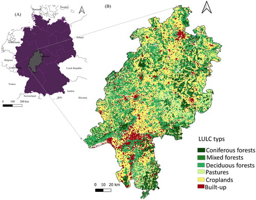
The state of Hesse is located in the centre of the Federal Republic of Germany. It has about 6.3 Million inhabitants, 2.4 Million people living in the Frankfurt-Rhine/Main region in the southern part of the federal state (Kallert et al., 2021). Outside the urbanized areas, the landscape is characterized by a high proportion of forests (ca. 42%), particularly in the northeast and east with forest cover up to 50% (HMUKLV 2023), but also intensively used agricultural regions, eg in the Wetterau north of Frankfurt (Jauker et al. 2009) where forest cover drops down to 15% (HMUKLV 2023), or non-intensively used grasslands in the Lahn-Dill (Reger et al. 2009) or Rhön region (Klinger et al. 2019). In eastern Hesse, the highest mountain with almost 950 m a.s.l is in the Rhön, and the largest continuous basalt area in Europe is the Vogelsberg area (Leßmann et al. 2000). Hesse’s geological features include the crystalline Odenwald in the South, the expanse of the Rhenish Slate Mountains in the West, the extensive deposits from the Triassic period (Buntsandstein, Muschelkalk, Keuper) in the North, areas with volcanic rocks, like the above-mentioned Vogelsberg, and the regions where Tertiary and Quaternary sedimentary rocks are distributed, eg the upper Rhine valley in the South (Becker and Reischmann 2021). Small-scale farming is still widespread and cultivated land lies on the limestone uplands and on the loess soils of the river lowlands. Wheat is the most widely grown crop, followed by potatoes and sugar beets. Poultry, pigs and cattle are the main livestock (HLNUG 2023). Figure 1 shows the location of the federal state of Hessen in Germany and a CORINE Land Cover map from 2018 with a spatial resolution of 100 m (CLC 2018) taken from the Copernicus land portal to show different LULC types across Hesse. CORINE land cover maps can be considered a standard for land monitoring in Europe (Feranec et al. 2016)

Figure 1. (A) Location of the federal state of Hesse in Central Germany and (B) the CORINE Land cover map from 2018 (CLC 2018).

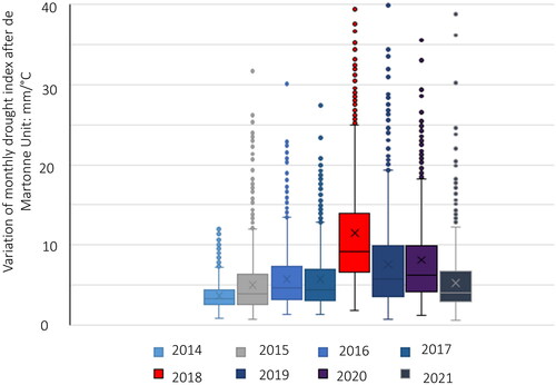
The climate of Hesse has rather continental features. The average rainfall is between 600 and 800 mm per year ranging from approximately 500 mm in the Upper Rhine Valley to as high as 1400 mm in elevated regions such as the Vogelsberg or the Rhön (HLNUG 2022a). The average annual temperature for the period 1981–2010 stands at 8.8 °C. This marks an increase from the previous period, 1951–1980, during which it was at 8.2 °C (HLNUG 2022a), and the trend shows that it continues to rise, i.e. up to 10.4 °C in 2020 (HLNUG 2020). Considerable variations in annual temperature can be observed, primarily oriented along a North-South axis (HLNUG 2022a, 2022b; Huebener et al. 2022). These variations range from minimal temperature changes in the northern regions to a notable 1.4 °C increase in the South (HLNUG 2022a). In addition, clear differences between urban (hot spots) and rural regions (cold spots) exist (HLNUG 2022b). The annual precipitation levels have also experienced a modest uptick, progressing from 735 mm (1901–1930) to 807 mm (1981–2010). According to the Climate Protection Scenario in Hesse, it is anticipated that average temperatures will continue to rise, leading to an increase in the number of particularly warm days with temperatures exceeding 30 °C (HLNUG 2022a). Nonetheless, there remains a possibility of occasional cold spells in winter and spring, including late frosts. Furthermore, precipitation maxima are expected to shift from summer to winter, with a greater likelihood of rain as opposed to snow during the winter season. Alongside changes in mean temperatures and precipitation, there is a projected increase in the probability and intensity of heavy precipitation events and droughts in the future (HLNUG 2018). In 2018, large parts of Europe including Hesse were affected by an extreme drought (Senf and Seidl 2021; Thonfeld et al. 2022; Beloiu et al. 2022). Such unprecedented hot droughts in Central Europe are expected to have strong effects, for example, on forest disturbance regimes (Senf and Seidl 2021). Furthermore, nine priority habitat types as defined by the European Habitats Directive (92/43/EEC) occur in Hesse, and seven of them are a likely to be negatively affected by climate change (Schwenkmezger 2019). According to the monthly drought index after de Martonne (CDC 2022), the year 2018 had the highest amount of variation of monthly drought from 2014 to 2021 in Hesse (Figure 2).

Figure 2. Variation of monthly drought index after de Martonne from 2014 to 2021 in Hesse/Germany (CDC 2022). maximum variation and drought happened in 2018.

2.2. Data and analysis

2.2.1. Dynamic Habitat Index (DHI)

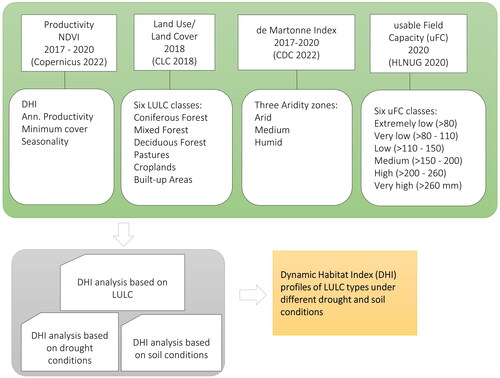
The flowchart in Figure 3 shows the conceptual framework of this study. The NDVI products of the Copernicus Global Land Service (Copernicus 2022) that are derived from top-of-canopy PROBA-V satellite data with 300 m spatial resolution (Copernicus 2022) were the basis to compute the three components of the DHI related to vegetation productivity. For this study, we used NDVI data from 01 January 2017 until 31 December 2020 with an interval of 10 days, which totalled up to 144 tiles for the full four-year dataset. For each year, the three DHI components were computed: cumulative DHI (${\mathit{DHI}\mathrm{ }}_{\mathit{Cum}}=\mathrm{ }\sum p_t$) indicating annual cumulative productivity, minimum DHI (${\mathit{DHI}}_{\min }=\min \hspace{0.17em}(p_t)$) indicating minimum cover and seasonality (${\mathit{DHI}}_{\mathit{Var}}=\frac{\sigma (p_t)}{\mathrm{\mu }\left(p_t\right)\mathrm{ }}$) based on the coefficient of variation using the standard deviation and the mean (p represents vegetation productivity at different periods (t)). The DHI_Total was generated from the composite of these three components. All details on DHI calculation are described by Coops et al. (2008), Hobi et al. (2017), Michaud et al. (2012) and Razenkova et al. (2020).

Figure 3. Conceptual framework of the study. The green box contains all input data and their categories. The grey boxes show the methodological steps and analysis to reach the target in the yellow box.

2.2.2. Land use/Land cover (LULC)

The 2018 CORINE Land Cover data set was used to extract six major LULC types in Hesse: coniferous, mixed and deciduous forests, pastures, croplands and built-up areas and a spatial resolution of 100 m (CLC 2018) using ‘Raster’ and ‘SF’ packages in R statistical software version 4 (R Core Team 2021)for raster and vector analysis. To visually control each LULC, the LULC maps and digital orthophotos (DOP) with 20 cm spatial resolution were overlaid (Geoportal Hessen 2022) in QGIS ver. 3.22 LTR Białowieża (QGIS Development Team 2021) (Figure 1(C)).

2.2.3. Precipitation conditions: de Martonne Index (dMI)

The de Martonne Index (dMI) is based on the relationship of precipitation and temperature for a given area ($\mathit{dMI}=\frac{P}{T+10}$ where T refers to the temperature in degrees Celsius and P refers to the precipitation in mm (de Martonne 1942). Low dMI values indicate aridity while increased values indicate humidity. Thus, the dMI provides information on the drought level at a given site and reflect the aridity of regional climate zones (Bhuyan et al. 2017) and has been used before in Central Germany to describe the extreme drought conditions in summer 2018 (Beloiu et al. 2022). We used monthly grids of the dMI from 01.01.2017 until 31.12.2020 provided by the German Climate Data centre (CDC 2022) to generate regional aridity zones map at 1 km spatial resolution based on a total of 48 tiles for the full four-year dataset (CDC 2022). To do so, we defined three aridity zones (arid, medium, humid) based on cumulative drought in the study area (dMI_Cum) for four years using the equation ${\mathit{dMI}}_{\mathit{Cum}}=\mathrm{ }\sum {\mathit{dMI}}_t,$ where It refers to the cumulative drought for period t. We used the ‘Raster’ package to calculate the dMI_Cum in R statistical software version 4 (R Core Team 2021). We then used natural break (Jenks), which accounts for non-uniform distributions and gives an unequal class width with varying frequency of observations per class, to identify the aridity zones.

2.2.4. Soil conditions: usable field capacity (uFC)

Spatial data on usable Field Capacity (uFC) data was used to study the variation of the DHI across different soil conditions (Table 1). The term field capacity is interchangeably used with the term water holding capacity and refers to the amount of water content held in soil after drainage of excess water (Rai et al. 2017). The uFC of a soil or a horizon describes the available part of the field capacity for vegetation. It thus includes the amount of water that a soil can retain against gravity. The data at a scale of 1:50 000 and a reference depth of 1 m were provided as vector data by Hessian State Agency for Nature Conservation, Environment and Geology (HLNUG_BFD50 2020). There are six main groups of uFC in Hessen ranging from very low to (0–80 mm) to very high (>260 mm) (Table 1). The highest coverage mainly belonged to low uFC (>110–150 mm) with almost 38% of the area, followed by medium uFC (>150–200 mm) with 26% and high uFC (>200–260 mm) with 16.5% of the area.

Table 1. Overview of the different usable field capacity (uFC) categories and the proportional areas in Hesse based on data by HLNUG_BFD(50 2020).

Usable field capacity categories	Level	Area (m^2)	Proportional area in Hesse
Extremely low	0–80 mm	567,495,992	2.99
Very low	>80–110 mm	2,831,954,494	14.95
Low	>110–150 mm	7,199,682,409	38.00
Medium	>150–200 mm	4,885,629,371	25.79
High	>200–260 mm	3,125,752,490	16.50
Very high	>260 mm	3,337,636,467	1.76

To answer the question whether the DHIs are susceptible to changes in soil conditions, we extracted the DHI component values across the six uFC categories for each LULC type in QGIS. When extracting the raster data including the DHIs based on vector categories such as uFC and LULC, pixels smaller than the native DHI pixel size (300 m) at the border of each vector were excluded. For each zone and LULC type the values for the three DHI components were extracted to explore whether the DHI is sensitive towards changing precipitation regimes across LULC types.

We also examined whether yearly DHI components from 2017 to 2020 differed across LULCs and whether they returned to their previous state after the severe drought in 2018. To test it, one-way analysis of variance (ANOVA) and post hoc Tukey test (p value <.05) was employed using the ‘car’ package (R Core Team 2021). Normality of data was checked using the Shapiro-Wilk test and the Q-Q plot of residuals, and Bartlett’s Test was used to check the equality of variances (Zuur et al. 2009).

3. Results

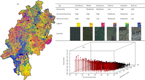
All LULC revealed distinct DHI profiles (Figure 4) in terms of annual productivity, minimum cover and seasonality. In the map, the colour patterns refer to different amounts of productivity and we could differentiate LULCs visually using digital orthophotos with 20 cm spatial resolution (Geoportal Hessen 2022). For example, blue colour indicates the built-up areas with low annual productivity, low minimum cover and high seasonality. The yellow areas are coniferous forests that are characterized by high annual productivity and minimum cover, but low seasonality. On the other hand, pastures with purple colour have intermediate annual productivity and minimum cover, but low seasonality (Figure 4(A,B)). The three-dimensional scatterplot indicates that the areas with high seasonality have lower annual productivity and minimum cover than the areas with low seasonality (Figure 4(C)).

Figure 4. The combined components of the dynamic habitat index derived from 2017 to 2020 (a). this composite image was developed by assigning the annual productivity to the red band, the minimum cover to the green band and the seasonality to the blue band. Blue areas have low annual productivity, low minimum cover and high seasonal variability. Thus, blue areas indicate the locations of the built-up areas. Bright yellow areas have a high annual productivity, a high minimum cover and low variability and represent locations with coniferous forests that were consistently green throughout the year. Purple areas or pastures indicate landscapes with medium annual productivity, medium minimum cover and low variability. Green areas or croplands indicate moderate landscape greenness that varies throughout the year. Red areas or deciduous forest have high annual production, moderate minimum cover and high seasonality. Black points on the map refer to the example areas (B) the three-dimensional scatterplot indicates three components of the DHI. The areas with high seasonality have lower annual productivity and minimum cover than the areas with low seasonality.

3.1. Response of the DHI to drought across LULC types

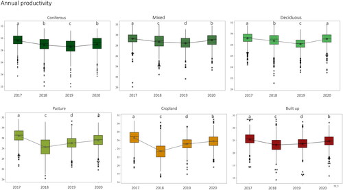
From 2017 to 2020, the annual productivity (DHI_Cum) for all LULCs had their maximum in 2017 (Figure 5). In 2018 and 2019, the annual productivity decreased for all LULC types and then started to recover. Except for deciduous forests, none of the other LULCs had fully returned to the pre-drought conditions in 2017. The highest values of annual productivity belonged to forests and pastures (range from 28 to 30) and built-up areas revealed the lowest annual productivity (range from 23 to 25).

Figure 5. Cumulative annual productivity (DHI_Cum) from 2017 to 2020 including the severe drought year 2018 for the six main Land use/Land Cover types in Hesse, Germany, namely, coniferous, mixed and deciduous forests, pastures, croplands and built-up areas. The black line connects the median of annual productivity. Small letters on the columns indicate significant differences in values based on one-way analysis of variance (ANOVA) and the Tukey post hoc test.

Minimum cover increased from 2018 to 2019 for all LULC types, and, in general, the highest values of DHI_Min belonged to the forest types (Figure 6). The highest values of minimum cover occurred in the drought year, which contrasts the output of DHI_Cum.

Figure 6. Minimum cover (DHI_Min) from 2017 to 2020 including the severe drought year 2018 for the six main Land use/Land Cover types in Hesse, Germany, namely, coniferous, mixed and deciduous forests, pastures, croplands and built-up areas. The black line connects the medians of minimum cover. Small letters on the columns indicate significant differences in values based on one-way analysis of variance (ANOVA) and the Tukey post hoc test.

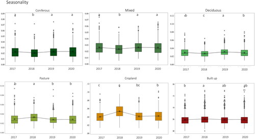
Forests and pastures showed less seasonality than croplands and built-up areas (Figure 7). After the drought 2018, the seasonality of the forest LULC types increased. In pastures and croplands, most variation occurred in 2018. In the built-up areas, seasonality was almost constant over the years.

Figure 7. Seasonality (DHI_Var) from 2017 to 2020 including the severe drought year 2018 for the six main Land use/Land Cover types in Hesse, Germany, namely, coniferous, mixed and deciduous forests, pastures, croplands and built-up areas. The black line connects the medians of seasonality. Small letters on the columns indicate significant differences in values based on one-way analysis of variance (ANOVA) and the Tukey post hoc test.

3.2. Effect of aridity zones on DHI components across LULC types

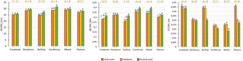
In general, for all LULC types, annual productivity and minimum cover were significantly higher than in the humid zone than in the medium and arid zone (Figure 8(A,B), p < .05). On the other hand, seasonality in arid zones was significantly higher compared to the other two zones (Figure 8(C), p < .05). More precisely, the annual productivity in the three forest types, pasture and built-up areas was significantly higher in the humid zone, but there is no significant difference between the medium and arid zone of coniferous and mixed forests and built-up areas (Figure 8(A)). In terms of minimum cover, again the highest values for all LULC types were observed in the humid zone (Figure 8(B)). The maximum seasonality mainly occurred in the arid zone in all LULCs (Figure 8(C)) and the seasonality in forest LULC types was less pronounced than that of pastures, croplands and built-up areas.

Figure 8. The three components of the Dynamic Habitat Index (DHI), namely (A) DHI_Cum (annual productivity), (B) DHI_Min (minimum cover) and (C) DHI_Var (seasonality) based on NDVI data from 2017 to 2020 are shown for six LULC types (coniferous, mixed and deciduous forests, pastures, croplands and built-up areas) and three aridity zones. The orange columns represent the arid zone, the yellow columns represent the medium zone, and the green columns represent the humid zone. The capital letter above the graph indicates the significance of the comparisons within each aridity zone separately, and the small letters inside the graph indicate the significance of the comparisons within each LULC type (p value <.05).

3.3. Effect of uFC on DHI components across LULC types

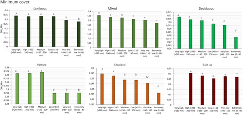
With decreasing uFC, annual productivity decreased in all LULC types except built-up areas (Figure 9(A)). In forest types, pasture and croplands lowest annual productivity was obtained for extremely low (0–80 mm) and very low (>80–110 mm) uFC, whereas maximum annual productivity values were obtained for high (>200–260 mm) and very high (>260 mm) uFc. In built-up areas, annual productivity was not affected by uFc (Figure 9(A)).

Figure 9. (A) Annual productivity (DHI_Cum), (B)​ minimum cover (DHI_min) and (C) seasonality (DHI_Var) of each LULC type (namely, coniferous, mixed and deciduous forests, pastures, croplands and built-up areas) depending on the usable field capacity (uFC). Small letters on the columns indicate significant differences between uFC classes (p value < .05).

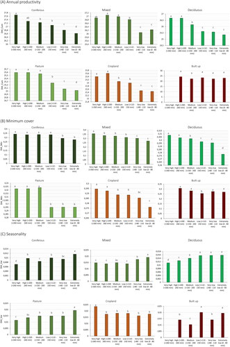
In terms of minimum cover, except of built-up areas, a decreasing trend was observed with decreasing uFC (Figure 9(B)). In forest types, pasture and croplands, the maximum values of minimum cover occurred in the areas with highest uFC.

Seasonality showed a trend opposite to the previous two DHI components. Thus, in forests and pastures lowest seasonality occurred where the uFC was the highest (>260 mm) and seasonality increased when uFC decreased (Figure 9(C)). Cropland and built-up areas showed different trends. For croplands, seasonality was higher in areas with very high uFC (>260 mm), while for built-up areas the changes were not in a particular order.

4. Discussion

We found that all LULC types had distinct and plausible DHI profiles (eg high productivity and minimum cover, but low intra-seasonal variability for all forest LULC types) that differed due to regional environmental changes related to soil and drought conditions. Annual productivity and seasonality clearly captured the response of the LULC types to different uFC classes and aridity zones, but minimum cover had different temporal trends. Indeed, heat stress and disturbances associated with droughts affect water availability in soil and reduce vegetation productivity (Xu et al. 2019), which is in line with the response of the DHI components to changing climatic and soil conditions. Therefore, the DHI provided a continuous measure to characterize LULC types which could provide more direct connections to ecosystem functions and health than purely static classifications (Coops and Wulder 2019). So, we see potential for composite vegetation indices or other land surface phenological products derived from satellite time-series data to complement common LULC maps to allow for a more detailed analysis of links between LULC and ecosystem functioning and services.

The DHI components responded to the severe drought year 2018. The DHI_Cum showed that apart from the deciduous forest none of the LULC types had returned to their original level after the drought event, which could be a sign of weakened resilience and vegetation degradation (Lloret et al. 2022; Manrique-Alba et al. 2022). Indeed, forests are facing several drought events with different intensities and magnitudes during their lifetime and therefore resilience to dry conditions may be critical to long-term survival (DeSoto et al. 2020). Understanding forest productivity and its variation under different environmental conditions is important especially when climate change is likely to strongly affect the productivity of temperate European forests (Morin et al. 2018). Capturing the effect of current droughts based on DHI in the forests can be a promising proxy to assess future tree mortality risk (eg by identifying DHI profiles of forests typical for die-off), especially when producing the DHI using high-resolution optical data like Planet Scopes or Rapid eye images (Silveira et al. 2023). However, the computation of the DHI with a relatively large pixel size comparable to the initial study by Coops et al. (2008) allows retrospective studies, for example using MODIS satellite data. In cases where the use of the NDVI might be limited, for example in semi-arid regions where vegetation cover is low or in the Tropics where the NDVI tends to saturate, other vegetation indices that can partially overcome these limitations such as the Enhanced Vegetation Index or the Soil-Adjusted Vegetation Index (Pettorelli et al. 2005) could be tested. Another alternative could be a biophysical parameter such as the LAI, which has been used in combination with precipitation indices for vegetation drought monitoring (Kim et al. 2017) and which has been computed in DHI studies (Hobi et al. 2017). A further limitation of using vegetation indices derived from passive optical remote sensing data might be the presence of clouds (Pettorelli et al. 2005). Latest development in forest drought monitoring includes the use of freely available SAR data (Kaiser et al. 2022; Schellenberg et al. 2023), so further potential exists to improve the power of DHI to detect and interpret changes or ecosystem degradation using high-temporal resolution active remote sensing data.

The integration of the DHI with spatial environmental information provides a more comprehensive understanding of ecosystem dynamics at the landscape scale (Michaud et al. 2012), which is extremely valuable for biodiversity assessments (Razenkova et al. 2023; Silveira et al. 2023). In addition, NDVI-based measurements from space have the potential to identify site-specific and climate-induced degradation of vegetation health (Margalef‐Marrase et al. 2020), but productivity related effects might show time lags of one to two years (Ogle et al. 2015), so combining the DHI with abiotic factors has the potential to provide insight into ecosystem degradation. Such integrated products could help decision makers to develop sustainable land management strategies and contribute to Sustainable Develop Goal (SDG) indicators such as SDG 15.3.1 that is related to land degradation (Sims et al. 2021), eg by identifying deviations of a LULC type from its typical DHI profile within its environmental context as a response to disturbance and environmental stress. Here, examining uFC for different LULCs revealed decreasing annual productivity with decreasing water holding capacity of the soil for all LULCs except built-up areas. The DHI was also able to clearly capture forest and pasture productivity depending on the uFC. Availability of more water is essential for forest growth and thus production, particularly in the context of global change and increased probabilities of severe droughts (Piedallu et al. 2011). In croplands, uFC can have a significant impact on the efficiency of crop productivity under given climate conditions (Fang and Su 2019; He and Wang 2019), and in this study, the DHIs were able to capture such variation. Due to management in croplands (ploughing) and intensive human activities in built-up areas (sealing) the seasonality was higher, and annual productivity was lower compared to forests and pastures. A reason for almost no differences in the built-up area could be the relatively large pixel size as fine urban landscape structures might require spectral unmixing approaches to map urban vegetation greenness even from Landsat time series data (Czekajlo et al. 2020), or the use of very high-resolution Planet Scope imagery (Silveira et al. 2023). On the other hand, the seasonality of urban heat islands has been mapped using a MODIS-based data product (Sismanidis et al. 2022). Quantifying sealed surfaces and their effect on productivity has been emphasized since it is important in a wide range of strategies to reduce impervious surfaces and their impacts on water resources and vegetation cover for site-level planning and land use regulation (Arnold and Gibbons 1996). Thus, future avenues of research particularly for urban areas could include the combination of the DHI based on the NDVI (or similar parameters) with high temporal thermal remote sensing data.

5. Conclusion

We show that composite remote sensing indices such as the DHI based on NDVI time series data are useful to characterize LULC types including their variation due to changing soil and drought conditions including effects of severe drought years in Central European landscapes. We argue that DHIs are an appropriate metric to complement or even replace discrete and static LULC maps especially for biodiversity and ecosystem research and application, for example within the frame of Sustainable Development Goals related to sustainable use of terrestrial ecosystems and ongoing land degradation such as SDG 15. Limitations due to coarse spatial resolution could be solved in the future due the availability of free high resolution optical satellite data, and the integration with high temporal resolution thermal and SAR satellite data is to our knowledge still underexplored. The methodological approach was based on publicly available data as well as free and open-source software, so we see potential for further studies in the field of monitoring impacts of climate change, landscape planning and management of ecosystems.

Disclosure statement

No potential conflict of interest was reported by the author(s).

Data availability statement

Data are available on request from the authors.

References

- Aghsaei H, Dinan NM, Moridi A, Asadolahi Z, Delavar M, Fohrer N, Wagner PD. 2020. Effects of dynamic land use/land cover change on water resources and sediment yield in the Anzali wetland catchment, Gilan, Iran. Sci Total Environ. 712:136449. doi: 10.1016/j.scitotenv.2019.136449.
- Akodéwou A, Oszwald J, Saïdi S, Gazull L, Akpavi S, Akpagana K, Gond V. 2020. Land use and land cover dynamics analysis of the Togodo protected area and its surroundings in Southeastern Togo, West Africa. Sustainability. 12(13):5439. doi: 10.3390/su12135439.
- Arnold CL, Gibbons CJ. 1996. Impervious surface coverage: the emergence of a key environmental indicator. J Am Plan Assoc. 62(2):243–258. doi: 10.1080/01944369608975688.
- Avand M, Moradi H, Lasboyee MR. 2021. Using machine learning models, remote sensing, and GIS to investigate the effects of changing climates and land uses on flood probability. J Hydrol. 595:125663. doi: 10.1016/j.jhydrol.2020.125663.
- Becker R, Reischmann T. 2021. Geologie von Hessen. Wiesbaden: Hessisches Landesamt für Naturschutz, Umwelt und Geologie (HLNUG).
- Belay T, Melese T, Senamaw A. 2022. Impacts of land use and land cover change on ecosystem service values in the Afroalpine area of Guna Mountain, Northwest Ethiopia. Heliyon. 8(12):e12246. doi: 10.1016/j.heliyon.2022.e12246.
- Beloiu M, Stahlmann R, Beierkuhnlein C. 2022. Drought impacts in forest canopy and deciduous tree saplings in Central European forests. For Ecol Manage. 509:120075. doi: 10.1016/j.foreco.2022.120075.
- Bhuyan U, Zang C, Menzel A. 2017. Different responses of multispecies tree ring growth to various drought indices across Europe. Dendrochronologia. 44:1–8. doi: 10.1016/j.dendro.2017.02.002.
- [CDC] Climate Data Center. 2022. Climate Data Center, Grids of monthly drought index (de Martonne) over Germany, version v1.0. [accessed 2021 August 23]. Index of/climate_environment/CDC/grids_germany/monthly/drought_index/(dwd.de).
- Chaves M, Picoli M, Sanches I. 2020. Recent applications of Landsat 8/OLI and Sentinel-2/MSI for land use and land cover mapping: a systematic review. Remote Sens. 12(18):3062. doi: 10.3390/rs12183062.
- [CLC] CORINE Land Cover. 2018. Copernicus land monitoring service (CLMS). Copenhagen K: European Environment Agency (EEA).
- Coops NC, Kearney SP, Bolton DK, Radeloff VC. 2018. Remotely-sensed productivity clusters capture global biodiversity patterns. Sci Rep. 8(1):16261. doi: 10.1038/s41598-018-34162-8.
- Coops NC, Wulder MA. 2019. Breaking the habit(at). Trends Ecol Evol. 34(7):585–587. doi: 10.1016/j.tree.2019.04.013.
- Coops NC, Wulder MA, Duro DC, Han T, Berry S. 2008. The development of a Canadian dynamic habitat index using multi-temporal satellite estimates of canopy light absorbance. Ecol Indic. 8(5):754–766. doi: 10.1016/j.ecolind.2008.01.007.
- Copernicus. 2022. Normalized difference vegetation index, Copernicus global land service, providing bio-geophysical products of global land surface. [accessed 2023 August 31]. https://land.copernicus.eu/global/products/ndvi.
- Czekajlo A, Coops NC, Wulder MA, Hermosilla T, Lu Y, White JC, van den Bosch M. 2020. The urban greenness score: a satellite-based metric for multi-decadal characterization of urban land dynamics. Int J Appl Earth Obs Geoinf. 93:102210. doi: 10.1016/j.jag.2020.102210.
- DeSoto L, Cailleret M, Sterck F, Jansen S, Kramer K, Robert EMR, Aakala T, Amoroso MM, Bigler C, Camarero JJ, et al. 2020. Low growth resilience to drought is related to future mortality risk in trees. Nat Commun. 11(1):545. doi: 10.1038/s41467-020-14300-5.
- de Martonne E. 1942. Nouvelle carte mondiale de l’indice d’aridite. Ann Geogr. 51(288):241–250. doi: 10.3406/geo.1942.12050.
- Fang J, Su Y. 2019. Effects of soils and irrigation volume on maize yield, irrigation water productivity, and nitrogen uptake. Sci Rep. 9(1):7740. doi: 10.1038/s41598-019-41447-z.
- Fathi-Taperasht A, Shafizadeh-Moghadam H, Sadian A, Xu T, Nikoo MR. 2023. Drought-induced vulnerability and resilience of different land use types using time series of MODIS-based indices. Int J Disaster Risk Reduct. 91:103703. doi: 10.1016/j.ijdrr.2023.103703.
- Feranec T, Soukup G, Hazeu G. 2016. European landscape dynamics. Corine land cover data. Boca Raton (FL): CRC-Press.
- Gashaw T, Tulu T, Argaw M, Worqlul AW, Tolessa T, Kindu M. 2018. Estimating the impacts of land use/land cover changes on Ecosystem Service Values: the case of the Andassa watershed in the Upper Blue Nile basin of Ethiopia. Ecosyst Serv. 31:219–228. doi: 10.1016/j.ecoser.2018.05.001.
- Gemitzi A, Banti MΑ, Lakshmi V. 2019. Vegetation greening trends in different land use types: natural variability versus human-induced impacts in Greece. Environ Earth Sci. 78(5):172. doi: 10.1007/s12665-019-8180-9.
- Geoportal Hessen. 2022. Hessische Verwaltung für Bodenmanagement und Geoinformation. Metadaten (hessen.de). [accessed 2022 February 15]. https://www.geoportal.hessen.de/.
- Haberstroh S, Werner C, Grün M, Kreuzwieser J, Seifert T, Schindler D, Christen A. 2022. Central European 2018 hot drought shifts scots pine forest to its tipping point. Plant Biol. 24(7):1186–1197. doi: 10.1111/plb.13455.
- He D, Wang E. 2019. On the relation between soil water holding capacity and dryland crop productivity. Geoderma. 353:11–24. doi: 10.1016/j.geoderma.2019.06.022.
- [HLNUG] Hessisches Landesamt für Naturschutz, Umwelt und Geologie. 2018. Klimawandel in Hessen. Wiesbaden: Hessisches Landesamt für Naturschutz, Umwelt und Geologie (HLNUG), Fachzentrum Klimawandel und Anpassung.
- [HLNUG] Hessisches Landesamt für Naturschutz, Umwelt und Geologie. 2020. Gewässerkundlicher Jahresbericht 2020. Hydrologie in Hessen 23. Wiesbaden: Hessisches Landesamt für Naturschutz, Umwelt und Geologie (HLNUG).
- [HLNUG] Hessisches Landesamt für Naturschutz, Umwelt und Geologie. 2022a. Beobachteter Klimawandel. Klimawandel in Hessen. Wiesbaden: Hessisches Landesamt für Naturschutz, Umwelt und Geologie (HLNUG).
- [HLNUG] Hessisches Landesamt für Naturschutz, Umwelt und Geologie. 2022b. Satellitenfernerkundung in Hessen. Mit Hitzekarten Hessens Hot Spots erkennen. Wiesbaden: Hessisches Landesamt für Naturschutz, Umwelt und Geologie (HLNUG).
- [HLNUG] Hessisches Landesamt für Naturschutz, Umwelt und Geologie. 2023. Hessisches Ministerium für Umwelt, Landwirtschaft und Forsten Geologische Entwicklung in Hessen. [accessed 2023 August 31]. https://www.hlnug.de/themen/geologie/geo-info-hessen/geologische-entwicklung-in-hessen/naturraum.
- HLNUG_BFD50. 2020. Nutzbare Feldkapazität des Bodens. Wiesbaden: Hessisches Landesamt für Naturschutz, Umwelt und Geologie (HLNUG).
- [HMUKLV] Hessisches Ministerium für Umwelt, Klimaschutz, Landwirtschaft und Verbraucherschutz. 2023. Naturnah & vielfältig. Wir machen den Wald klimastabil. Hessisches Ministerium für Umwelt, Klimaschutz, Landwirtschaft und Verbraucherschutz (HMUKLV); [accessed 2023 October 9]. https://umwelt.hessen.de/wald.
- Hobi ML, Dubinin M, Graham CH, Coops NC, Clayton MK, Pidgeon AM, Radeloff VC. 2017. A comparison of Dynamic Habitat Indices derived from different MODIS products as predictors of avian species richness. Remote Sens Environ. 195:142–152. doi: 10.1016/j.rse.2017.04.018.
- Huebener H, Gelhardt U, Lang J. 2022. Improved representativeness of simulated climate using natural units and monthly resolution. Front Clim. 4:991082. doi: 10.3389/fclim.2022.991082.
- Jauker F, Diekötter T, Schwarzbach F, Wolters V. 2009. Pollinator dispersal in an agricultural matrix: opposing responses of wild bees and hoverflies to landscape structure and distance from main habitat. Landscape Ecol. 24(4):547–555. doi: 10.1007/s10980-009-9331-2.
- Kaiser P, Buddenbaum H, Nink S, Hill J. 2022. Potential of Sentinel-1 data for spatially and temporally high-resolution detection of drought affected forest stands. Forests. 13(12):2148. doi: 10.3390/f13122148.
- Kallert A,Belina B,Miessner M,Naumann M. 2021. The cultural political economy of rural governance: regional development in Hesse (Germany). J Rural Stud. 87:327–337. doi: 10.1016/j.jrurstud.2021.09.017.
- Karra K, Kontgis C, Statman-Weil Z, Mazzariello CJ, Mathis M, Brumby SP. 2021. Global land use/land cover with Sentinel 2 and deep learning. In: 2021 IEEE International Geoscience and Remote Sensing Symposium IGARSS; Jul 11–16; Brussels, Belgium. IEEE. p. 4704–4707. doi: 10.1109/IGARSS47720.2021.9553499.
- Kim K, Wang MC, Ranjitkar S, Liu SH, Xu JC, Zomer RJ. 2017. Using leaf area index (LAI) to assess vegetation response to drought in Yunnan province of China. J Mt Sci. 14(9):1863–1872. doi: 10.1007/s11629-016-3971-x.
- Klinger YP, Harvolk-Schöning S, Eckstein RL, Hansen W, Otte A, Ludewig K. 2019. Applying landscape structure analysis to assess the spatio-temporal distribution of an invasive legume in the Rhön UNESCO Biosphere Reserve. Biol Invasions. 21(8):2735–2749. doi: 10.1007/s10530-019-02012-x.
- Kooistra L, Berger K, Brede B, Graf LV, Aasen H, Roujean J-L, Machwitz M, Schlerf M, Atzberger C, Prikaziuk E. 2023. Reviews and syntheses: remotely sensed optical time series for monitoring vegetation productivity. Biogeosci Discuss. 2023:1–67. doi: 10.5194/bg-2023-88.
- Le TDH, Pham LH, Dinh QT, Hang NTT, Tran TAT. 2022. Rapid method for yearly LULC classification using Random Forest and incorporating time-series NDVI and topography: a case study of Thanh Hoa province, Vietnam. Geocarto Int. 37(27):17200–17215. doi: 10.1080/10106049.2022.2123959.
- Leßmann B, Scharpff H-J, Wedel A, Wiegand K. 2000. Grundwasser im Vogelsberg, Wiesbaden, Germany: Hessisches Ministerium für Umwelt, Landwirtschaft und Forsten. [accessed 2023 August 31]. https://www.hlnug.de/fileadmin/dokumente/wasser/hydrogeologie/grundwasser_im_vogelsberg.pdf.
- Lloret F, Jaime LA, Margalef-Marrase J, Pérez-Navarro MA, Batllori E. 2022. Short-term forest resilience after drought-induced die-off in Southwestern European forests. Sci Total Environ. 806(Pt 4):150940. doi: 10.1016/j.scitotenv.2021.150940.
- Mackey B, Bryan J, Randall L. 2004. Australia’s dynamic habitat template 2003. Proceedings of the MODIS Vegetation Workshop II, Apr 17; Missoula, MT: American.
- Manrique-Alba À, Beguería S, Camarero JJ. 2022. Long-term effects of forest management on post-drought growth resilience: an analytical framework. Sci Total Environ. 810:152374. doi: 10.1016/j.scitotenv.2021.152374.
- Margalef‐Marrase J, Pérez‐Navarro MÁ, Lloret F. 2020. Relationship between heatwave‐induced forest die‐off and climatic suitability in multiple tree species. Glob Chang Biol. 26(5):3134–3146. doi: 10.1111/gcb.15042.
- Marshall L, Biesmeijer JC, Rasmont P, Vereecken NJ, Dvorak L, Fitzpatrick U, Francis F, Neumayer J, Ødegaard F, Paukkunen JPT, et al. 2018. The interplay of climate and land use change affects the distribution of EU bumblebees. Glob Chang Biol. 24(1):101–116. doi: 10.1111/gcb.13867.
- Mas J-F, Lemoine-Rodríguez R, González-López R, López-Sánchez J, Piña-Garduño A, Herrera-Flores E. 2017. Land use/land cover change detection combining automatic processing and visual interpretation. Eur J Remote Sens. 50(1):626–635. doi: 10.1080/22797254.2017.1387505.
- Michaud J-S, Coops NC, Andrew ME, Wulder MA. 2012. Characterising spatiotemporal environmental and natural variation using a dynamic habitat index throughout the province of Ontario. Ecol Indic. 18:303–311. doi: 10.1016/j.ecolind.2011.11.027.
- Morin X, Fahse L, Jactel H, Scherer-Lorenzen M, García-Valdés R, Bugmann H. 2018. Long-term response of forest productivity to climate change is mostly driven by change in tree species composition. Sci Rep. 8(1):5627. doi: 10.1038/s41598-018-23763-y.
- Musetsho KD, Chitakira M, Nel W. 2021. Mapping land-use/land-cover change in a critical biodiversity area of South Africa. Int J Environ Res Public Health. 18(19):10164. doi: 10.3390/ijerph181910164.
- Ogle K, Barber JJ, Barron-Gafford GA, Bentley LP, Young JM, Huxman TE, Loik ME, Tissue DT. 2015. Quantifying ecological memory in plant and ecosystem processes. Ecol Lett. 18(3):221–235. doi: 10.1111/ele.12399.
- Pettorelli N, Vik JO, Mysterud A, Gaillard JM, Tucker CJ, Stenseth NC. 2005. Using the satellite-derived NDVI to assess ecological responses to environmental change. Trends Ecol Evol. 20(9):503–510. doi: 10.1016/j.tree.2005.05.011.
- Piedallu C, Gégout J-C, Bruand A, Seynave I. 2011. Mapping soil water holding capacity over large areas to predict potential production of forest stands. Geoderma. 160(3-4):355–366. doi: 10.1016/j.geoderma.2010.10.004.
- QGIS Development Team. 2021. QGIS geographic information system. Open source geospatial foundation project. [accessed 2021 October 30]. http://qgis.osgeo.org.
- Rai RK, Singh VP, Upadhyay A, Rai RK, Singh VP, Upadhyay A. 2017. Chapter 17 - soil analysis. In: Rai RK, Singh VP, Upadhyay A, editors. Planning and evaluation of irrigation projects [Internet]. [place unknown]: Academic Press; p. 505–523. doi: 10.1016/B978-0-12-811748-4.00017-0.
- Ramirez-Reyes C, Brauman KA, Chaplin-Kramer R, Galford GL, Adamo SB, Anderson CB, Anderson C, Allington GRH, Bagstad KJ, Coe MT, et al. 2019. Reimagining the potential of Earth observations for ecosystem service assessments. Sci Total Environ. 665:1053–1063. doi: 10.1016/j.scitotenv.2019.02.150.
- Razenkova E, Dubinin M, Pidgeon AM, Hobi ML, Zhu L, Bragina EV, Allen AM, Clayton MK, Baskin LM, Coops NC, et al. 2023. Abundance patterns of mammals across Russia explained by remotely sensed vegetation productivity and snow indices. J Biogeogr. 50(5):932–946. doi: 10.1111/jbi.14588.
- Razenkova E, Radeloff VC, Dubinin M, Bragina EV, Allen AM, Clayton MK, Pidgeon AM, Baskin LM, Coops NC, Hobi ML. 2020. Vegetation productivity summarized by the Dynamic Habitat Indices explains broad-scale patterns of moose abundance across Russia. Sci Rep. 10(1):836. doi: 10.1038/s41598-019-57308-8.
- R Core Team. 2021. R: a language and environment for statistical computing. Vienna: R Foundation for Statistical Computing.
- Reger B, Mattern T, Otte A, Waldhardt R. 2009. Assessing the spatial distribution of grassland age in a marginal European landscape. J Environ Manage. 90(9):2900–2909. doi: 10.1016/j.jenvman.2007.10.015.
- Runge J, Bathiany S, Bollt E, Camps-Valls G, Coumou D, Deyle E, Glymour C, Kretschmer M, Mahecha MD, Muñoz-Marí J, et al. 2019. Inferring causation from time series in Earth system sciences. Nat Commun. 10(1):2553. doi: 10.1038/s41467-019-10105-3.
- Safaei M, Bashari H, Kleinebecker T, Fakheran S, Jafari R, Große-Stoltenberg A. 2023. Mapping terrestrial ecosystem health in drylands: comparison of field-based information with remotely sensed data at watershed level. Landsc Ecol. 38(3):705–724. doi: 10.1007/s10980-022-01454-4.
- Safaei M, Bashari H, Mosaddeghi MR, Jafari R. 2019. Assessing the impacts of land use and land cover changes on soil functions using landscape function analysis and soil quality indicators in semi-arid natural ecosystems. CATENA. 177:260–271. doi: 10.1016/j.catena.2019.02.021.
- Schellenberg K, Jagdhuber T, Zehner M, Hese S, Urban M, Urbazaev M, Hartmann H, Schmullius C, Dubois C. 2023. Potential of Sentinel-1 SAR to assess damage in drought-affected temperate deciduous broadleaf forests. Remote Sens. 15(4):1004. doi: 10.3390/rs15041004.
- Schwenkmezger L. 2019. Auswirkungen des Klimawandels auf hessische Arten und Lebensräume: Liste potentieller Klimaverlierer. Wiesbaden: Hessisches Landesamt für Naturschutz, Umwelt und Geologie (HLNUG).
- Senf C, Seidl R. 2021. Persistent impacts of the 2018 drought on forest disturbance regimes in Europe. Biogeosciences. 18(18):5223–5230. doi: 10.5194/bg-18-5223-2021.
- Sharma R, Nehren U, Rahman SA, Meyer M, Rimal B, Aria Seta G, Baral H. 2018. Modeling land use and land cover changes and their effects on biodiversity in Central Kalimantan, Indonesia. Land. 7(2):57. doi: 10.3390/land7020057.
- Sharma R, Rimal B, Baral H, Nehren U, Paudyal K, Sharma S, Rijal S, Ranpal S, Acharya RP, Alenazy AA, et al. 2019. Impact of land cover change on ecosystem services in a tropical forested landscape. Resources. 8(1):18. doi: 10.3390/resources8010018.
- Sharma S, Hussain S, Singh AN. 2023. Impact of land use and land cover on urban ecosystem service value in Chandigarh, India: a GIS-based analysis. J Urban Ecol. 9(1):juac030. doi: 10.1093/jue/juac030.
- Silveira EMO, Pidgeon AM, Farwell LS, Hobi ML, Razenkova E, Zuckerberg B, Coops NC, Radeloff VC. 2023. Multi-grain habitat models that combine satellite sensors with different resolutions explain bird species richness patterns best. Remote Sens Environ. 295:113661. doi: 10.1016/j.rse.2023.113661.
- Sims NC, Newnham GJ, England JR, Guerschman J, Cox SJD, Roxburgh SH, Viscarra Rossel RA, Fritz S, Wheeler I. 2021. Good practice guidance. SDG indicator 15.3.1, proportion of land that is degraded over total land area. Version 2.0. Bonn: United Nations Convention to Combat Desertification. [accessed 2023 August 31]. https://www.unccd.int/ publications/good-practice-guidance-sdg-indicator-1531proportion-land-degraded-over-total-land.
- Sismanidis P, Bechtel B, Perry M, Ghent D. 2022. The seasonality of surface urban heat islands across climates. Remote Sens. 14(10):2318. doi: 10.3390/rs14102318.
- Suttidate N, Hobi ML, Pidgeon AM, Round PD, Coops NC, Helmers DP, Keuler NS, Dubinin M, Bateman BL, Radeloff VC. 2019. Tropical bird species richness is strongly associated with patterns of primary productivity captured by the dynamic habitat indices. Remote Sens Environ. 232:111306. doi: 10.1016/j.rse.2019.111306.
- Talukdar S, Singha P, Mahato S, Shahfahad, Pal S, Liou Y-A, Rahman A. 2020. Land-use land-cover classification by machine learning classifiers for satellite observations—a review. Remote Sens. 12(7):1135. doi: 10.3390/rs12071135.
- Thonfeld F, Gessner U, Holzwarth S, Kriese J, da Ponte E, Huth J, Kuenzer C. 2022. A first assessment of canopy cover loss in Germany’s forests after the 2018–2020 drought years. Remote Sens. 14(3):562. doi: 10.3390/rs14030562.
- Wagner PD, Bhallamudi SM, Narasimhan B, Kantakumar LN, Sudheer KP, Kumar S, Schneider K, Fiener P. 2016. Dynamic integration of land use changes in a hydrologic assessment of a rapidly developing Indian catchment. Sci Total Environ. 539:153–164. doi: 10.1016/j.scitotenv.2015.08.148.
- Xu C, McDowell NG, Fisher RA, Wei L, Sevanto S, Christoffersen BO, Weng E, Middleton RS. 2019. Increasing impacts of extreme droughts on vegetation productivity under climate change. Nat Clim Chang. 9(12):948–953. doi: 10.1038/s41558-019-0630-6.
- Yonaba R, Biaou AC, Koïta M, Tazen F, Mounirou LA, Zouré CO, Queloz P, Karambiri H, Yacouba H. 2021. A dynamic land use/land cover input helps in picturing the Sahelian paradox: assessing variability and attribution of changes in surface runoff in a Sahelian watershed. Sci Total Environ. 757:143792. doi: 10.1016/j.scitotenv.2020.143792.
- Yonaba R, Koïta M, Mounirou LA, Tazen F, Queloz P, Biaou AC, Niang D, Zouré C, Karambiri H, Yacouba H. 2021. Spatial and transient modelling of land use/land cover (LULC) dynamics in a Sahelian landscape under semi-arid climate in northern Burkina Faso. Land Use Policy. 103:105305. doi: 10.1016/j.landusepol.2021.105305.
- Zeng X, Hu Z, Chen A, Yuan W, Hou G, Han D, Liang M, Di K, Cao R, Luo D. 2022. The global decline in the sensitivity of vegetation productivity to precipitation from 2001 to 2018. Glob Chang Biol. 28(22):6823–6833. doi: 10.1111/gcb.16403.
- Zhang W, Wei F, Horion S, Fensholt R, Forkel M, Brandt M. 2022. Global quantification of the bidirectional dependency between soil moisture and vegetation productivity. Agric For Meteorol. 313:108735. doi: 10.1016/j.agrformet.2021.108735.
- Zhang Y, Wang K, Wang J, Liu C, Shangguan Z. 2021. Changes in soil water holding capacity and water availability following vegetation restoration on the Chinese Loess Plateau. Sci Rep. 11(1):9692. doi: 10.1038/s41598-021-88914-0.
- Zuur A, Leno EN, Walker N, Saveliev AA, Smith GM. 2009. Mixed effects models and extensions in ecology with R. New York: Springer.