Graph neural network-based identification of ditch matching patterns across multi-scale geospatial data

Abstract

Ditches are vital to water system data. To ease the task of matching multi-scale ditch data and enhance accuracy (Acc), it is essential to discern ditch data matching patterns. Despite its importance, limited research has been conducted on ditch matching patterns, and the primary reasons for variations in multi-scale geographical entities’ matching patterns remain underexplored. Here, we introduce a supervised graph neural network (GNN) method, targeting the direct analysis of 1:10,000 ditch characteristics to identify the matching patterns between 1:10,000 and 1:25,000 datasets. The ditch network is depicted as a graph structure, with nodes representing ditch segments and edges indicating their connections. Subsequently, each ditch segment’s geometric, semantic, and topological attributes are computed as node attributes, and their matching patterns with the 1:25,000 dataset are labeled as node annotations. Ditch segment matching patterns are then categorized using supervised learning. Experiments using Overijssel, Netherlands’ ditch data reveal that this method achieves a 97.3% classification Acc, outperforming other GNN methods by 25.6–26.3% and traditional machine learning methods by 33%. These findings underscore the efficacy and superiority of the proposed supervised GNN approach in pinpointing ditch matching patterns.

Keywords:

• Multi-scale integration
• spatial data matching
• matching pattern identification
• ditches
• graph neural networks

1. Introduction

Matching geospatial data is pivotal for multi-scale spatial data integration, fusion, scale transformation, and updating. It remains a core technology for maintaining the currency and accuracy (Acc) of established databases (Chehreghan and Ali Abbaspour, 2018; Zhang et al. 2022). Water system data constitute a significant component of geospatial databases and are a primary focus in the production and application of geographic data (Liu et al. 2021a, 2021b). Ditches, as typical linear water elements, efficiently drain rainwater, mitigating the risk of water disasters and floods. Commonly found in clusters in rural areas, they play a vital role in material transport and irrigation in agricultural regions, reflect farmland layouts, and influence the agro-ecosystem landscape (Sandro et al. 2011). The utilization of matching pattern identification in matching is prevalent, facilitating a reduction in matching complexity and enhancing both matching rates and Acc. A matching pattern delineates the correspondence between the number of same-name entities across different scales (Zhang et al. 2018). These same-name entities are spatial entities representing identical real-world objects across various data sources. Given the notable differences in geometric, semantic, and contextual features across scales, their matching patterns are diverse, typically categorized as 1:0, 1:1, 1:m and m:n (Zhang et al. 2018; Lei 2021; Yu and Liu 2023). Recognizing the matching pattern of same-name entities early in the ditch matching process can positively influence subsequent endeavors, making the matching process less complex and more accurate and efficient. This also facilitates scale transformation and updating, aligning more closely with the big data research paradigm in a machine learning environment.

Research on the matching of linear elements like road networks is more established, whereas studies on water system data matching remain limited (Zhong 2018). Additionally, most research on matching patterns has been subsumed under studies on matching methods, with few standalone investigations in recent years. Research methods for matching linear elements can be categorized as following. The first approach involves measuring the similarity between potential matching pairs using spatial or non-spatial parameters, followed by searching for matching results (Zhang et al. 2014; Chen et al. 2016; Liu et al. 2020). Simple search methods primarily employ geometric measurements for matching (Kim et al. 2010; Guo et al. 2019). For instance, Zhang et al. introduced a buffer-based algorithm that iteratively adjusts the buffer size for optimal matching (Zhang and Meng, 2007). Within this method, matching pattern identification calculates local similarities to attain matches that meet a similarity threshold, thereby determining the matching patterns of geographic entities. The precision (P) of this method hinges on the similarity threshold setting, making accurate pattern identification challenging. Complex search methods derive matching outcomes by measuring a combination of multiple indicators (Fu et al. 2016; Chehreghan and Ali Abbaspour, 2017; Gao et al. 2022), using techniques, such as machine learning (Liu et al. 2020), the genetic coding algorithm (Chehreghan and Ali Abbaspour, 2018) or the probability relaxation method (Zhang et al. 2018). During this process, after setting similarity feature combinations and weights, geographical entities with 1:0, 1:1 and 1:m matching patterns are initially identified. Subsequently, spatial domain division or virtual path connections are applied to the remaining unmatched entities to discern m:n matching patterns. The method requires significant prior knowledge to set appropriate weights and thresholds for similarity features, and improper configurations can influence the results. Another category is optimization-based matching, which employs constraint functions to find the best solution under specific criteria (Zhang et al. 2021). This method’s primary aim is to identify corresponding targets, not just measure similarity. Li and Goodchild (2011) framed the matching issue as an objective function aiming for an optimal value and incorporated the directed Hausdorff distance to address 1:1 and 1:m correspondences. Meanwhile, Tong integrated optimization with logistic regression models (Tong et al. 2014), and Wu introduced a minimum network flow optimization approach for many-to-many correspondences (Wu et al. 2022). In these techniques, the matching pattern is progressively refined from initial fuzzy results using filters like logistic regression models (Tong et al. 2014), angle constraints (Wu et al. 2022), path direction constraints (Wang, Liu, et al. 2023; Wang, Yan, et al. 2023) and more. Additionally, the interactive polyline matching approach determines matching patterns via structural similarity criteria (Yu and Liu 2023).

The studies mentioned previously have overlooked a significant factor influencing the diversity of matching patterns between geographic entities. This factor is the necessity for same-name entities in multi-scale spatial data production to undergo cartographic generalization operations due to varying map scales and data uses. Cartographic generalization employs various operations, such as selection, deletion and simplification, based on the geometric, semantic and topological attributes of the geographical entities. This results in variations of same-name entities across different scale databases, accounting for the diversity in matching patterns for these entities at varying scales.

This article takes a direct approach, focusing on the characteristics of multi-scale entities with the same name. Utilizing machine learning and data-driven techniques, we introduce a case-based graph neural network (GNN) method for matching pattern identification. This method aims to discern the matching patterns of same-name entities within 1:10,000 and 1:25,000 ditch datasets. In this approach, each ditch segment serves as a node within the graph structure. The GNN method adaptively learns the semantic, geometric, topological, and contextual features present in the ditch data. Consequently, the matching pattern for 1:10,000 ditch data in relation to 1:25,000 data is determined, facilitating the subsequent integration, matching, fusion, scale transformation and update of the 1:10,000 ditch data.

2. Graph representation of a ditch network and sample dataset construction

The discrepancy between the 1:10,000 and 1:25,000 ditch data arises from cartographic generalization during the data production phase. Thus, when identifying the 1:10,000 matching pattern, both the node feature design of the graph and the architecture of the network model must adequately account for the cartographic generalization operation. Given the significant utility of graphs in representing vector data information (Ai 2021; Yang, Kong, et al. 2022; Yang, Jiang, et al. 2022), the preprocessed ditch data is transformed into a graph structure, with node features derived from ditch segments.

2.1. Modeling a ditch network as a graph

The modeling and annotation of ditch networks based on graph structure are illustrated in Figure 1. Initially, ditches are segmented at intersection points and where the ditch width changes. Each of these segments acts as a node, with the interconnections between them being the edges. In practical scenarios, the intersection of ditches represents a graph node, while individual ditch segments are viewed as edges. Through the construction of the ditch data’s dual graph, each ditch segment becomes a graph node, enabling the extraction of rich node features while preserving the topological structure and attributes of the ditch network.

Figure 1. Graph modeling of a ditch network. (a) Original ditch network; (b) divided ditch segments; (c) graph structure representation.

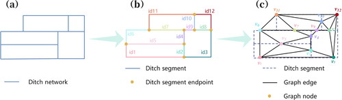
The dual graph of the ditch network employs graph theory to encapsulate the ditch network. It can be defined as follows: The nodes of the graph are the midpoints of each ditch segment and can be denoted as $G=(V,E,A);$ $\text{V=}\left\{v_0,v_1,v_2\dots v_{n-1}\right\}$ represents the set of nodes in the graph, i.e. the set of ditch segments; $E$ represents the edges linking the nodes, i.e. the connectivity between ditch segments; $A$ is an adjacency matrix indicating the edge weights between $n$ nodes, formulated based on their interrelationships. Within this matrix, a topological relationship between nodes results in a value of 1; if absent, the value is 0. Moreover, when utilizing GNN for node classification, only the connection relationship between nodes is taken into account, excluding any mutual relationships. Consequently, in this research, the dual graph of the ditch network is depicted as an undirected graph.

2.2. Feature extraction

In the generation of 1:10,000 and 1:25,000 ditch data, generalization operations are employed to reconcile scale differences and diverse data applications. Consequently, during the matching pattern identification process, features can be established based on cartographic generalization principles. During the cartographic generalization of linear water elements, various features have been predominantly utilized: geometric features (Duan et al. 2020; Zheng et al. 2021; Wang, Liu, et al. 2023; Wang, Yan, et al. 2023), semantic features (Zheng et al. 2021; Yang, Kong et al. 2022), topological features (Duan et al. 2020; Wang, Liu, et al. 2023; Wang, Yan, et al. 2023), and contextual features (Duan et al. 2019). To comprehensively represent the attributes of each ditch segment, this research also designs features from these domains and specifies the associated feature indicators, as outlined in Table 1.

Table 1. Graph node characteristics.

Class	Feature	Description
Geometric features	Length	Refers to the length of the ditch segment entity. A larger length value indicates a higher likelihood of retention in data generation.
Semantic features	Level	Refers to the hierarchy level of the ditch segment entity. Segments are divided based on width into levels 1, 2 and 3.
Topological features	Number of adjacent ditches (AdjaLoop)	Indicates the number of ditch segments connected to a given segment. A higher number suggests better connectivity.
	Whether connected to lakes (AdjaLake)	Specifies if the ditch segment connects to a lake, highlighting its geographical importance.
Contextual features	Maximum length (MaxLength)	Represents the length of the Stroke corresponding to the ditch segment.
	Value of betweenness centrality (Sbet)	Refers to the mediation centrality value of the Stroke associated with the ditch segment.
	Connectivity (Sconnect)	Describes the connectivity of the Stroke related to the ditch segment.
	Density of ditch networks (Density)	Indicates the distribution density of ditch segments in a specific area, serving as a fundamental contextual feature.

In this study, the ‘ditch Stroke’ is structured using semantic and angle constraints. The semantic constraint is defined by a consistent ‘level,’ while the angular constraint is established as greater than ‘135°’. The ditch network density is described by $D=L/A,$ $L$ signifies the length of other ditches falling within the buffer with an angle difference below the set threshold, and $A$ represents the area of the ditch buffer. Through iterative experimentation, it was found that setting the buffer threshold at 100 m and the angle threshold at 30° yielded the most detailed ditch network density information for each segment.

2.3. Node labeling

During node labeling, a combined manual and machine approach is utilized to discern the matching pattern of 1:10,000 data. Initially, the ditch data at both 1:10,000 and 1:25,000 scales undergo preprocessing. Utilizing expert insights, buffers are generated for the ditch data at these scales, and the overlap area between them is determined to facilitate the preliminary matching of same-name entities. Based on prior research and experimental findings, the overlap threshold is established at 90%. If the overlapping area between the two scale levels surpasses 90%, it is acknowledged as a successful preliminary match. Conversely, if it falls below 90%, the pre-match is deemed unsuccessful. Subsequent to this, the preliminary matching outcomes undergo manual verification to establish accurate matching relationships for same-name entities, as shown in Figure 2(a). Finally, according to the matching results, the matching mode of 1:10,000 data is determined, that is, the node annotation of the graph, as shown in Figure 2(b).

Figure 2. Graph node annotation. (a) Part of the matching results between 1:10,000 and 1:25,000 ditch data; (b) matching patterns of partial 1:10,000 ditch data.

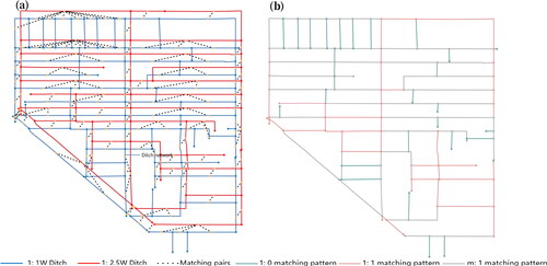
Given that the cartographic generalization interoperation between the 1:10,000 and 1:25,000 ditch data predominantly centers around selection, there are a scant number of m:n matching patterns present in the 1:10,000 ditch data. Recognizing that both the m:n and m:1 matching patterns of 1:10,000 data emerge post the identical cartographic generalization action (merge), and considering that the 1:10,000 data undergoes a ‘cancel line segmentation’ during preprocessing to effectively preclude the onset of m:n matching patterns, the m:n matching pattern data is consolidated into the m:1 category. Within this research, the recognition of ditch matching patterns is confined to 1:0, 1:1, and m:1.

2.4. Sample dataset construction

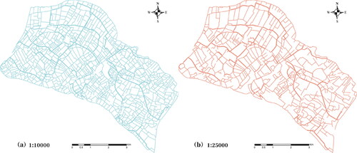
In this study, the Overijssel area of the Netherlands was selected as the experimental area to construct a sample database with a complex and complete artificial ditch network.Our initial step involved the removal of disorganized lines in the experimental area that lacked any connection relationship. We then connected the interrupted ditches and extracted the centerline of the faceted ditch to serve as our experimental subject. Subsequently, we carried out topological checks on the ditch data to ensure the absence of errors, such as false nodes or self-intersections. We segmented the comprehensive ditch network at intersection points and points where ditch width varied, yielding 3275 ditch segments at a 1:10,000 scale and 1225 segments at a 1:25,000 scale (refer to Figure 3).

Figure 3. Experimental data. (a) Ditch data at 1:10,000 scale; (b) ditch data at 1:25,000 scale.

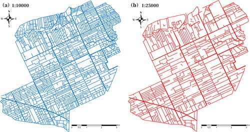
Upon executing the appropriate matching procedures, we isolated ditch data from the 1:10,000 segment dataset that adhered to specific matching patterns. To be precise, the data comprised 1161 segments with a 1:0 matching pattern, 772 segments with a 1:1 pattern and 1342 segments with an m:1 pattern. Concurrently, we partitioned the dataset into training, validation and test subsets following an 8:1:1 ratio. As outlined in Section 2.2, we established a dual graph and node sample library based on ditch segments. This graph structure incorporates a total of 3275 nodes and 6429 edges, which will be employed as input layers for the ensuing training and testing phases.

3. Methodology

Graph sample and aggregate (GraphSAGE) and topological adaptive graph convolutional network (TAGCN) are two typical types of GNNs. Based on the convolution operation in GraphSAGE and TAGCN, the data graph and features are input (Section 2) to complete the matching pattern recognition of the ditch. Relevant evaluation indicators are introduced to evaluate the performance of the model.

3.1. GNN model construction for ditch matching pattern identification

Since vector data does not have a regular and ordered data structure, deep learning methods based on graph structures have stronger applicability to process such data than traditional machine learning methods. This is because vector data can be converted into a graph structure without losing feature information. Compared with other deep learning methods, GNNs pay more attention to the connection relationship between nodes, and can adaptively learn the representation of each node, so as to have stronger generalization performance in tasks such as classification and prediction.

GraphSAGE and TAGCN are two typical GNN types. GraphSAGE is an inductive spatial domain learning framework that extracts node neighborhood information from graphs through neighbor sampling and aggregate functions, which can represent nodes on large-scale graphs. The novelty of GraphSAGE resides in its sampling method, where the strategy aligns with the production process of ditch data. Specifically, during the cartographic generalization process, it emphasizes key neighboring information instead of the entire dataset. Considering that there are many nodes in the graph structure constructed in this study, the neighborhood characteristics of the nodes need to be taken into account in the matching pattern identification, so the GraphSAGE neural network is introduced for the matching pattern identification of ditches.

TAGCN is a model based on a graph convolutional neural network (GCN), which uses a graph convolutional layer to extract node features and enhance the representation ability of nodes by skipping connections so as to have stronger generalization performance when processing complex graph data. Implementing TAGCN as a ‘classifier’ in the model predominantly takes into account two aspects. First, compared to fully connected layers, TAGConv layers leverage the graph’s structural information more effectively, enhancing the mapping from ‘feature representation’ to the label space. Second, in contrast to traditional graph convolutional layers, the TAGConv layer captures information within neighbors of order. Given the discrete nature of ditch distribution, lines in proximity might not necessarily be immediate neighbors. However, these non-adjacent yet spatially interconnected lines are crucial for pattern identification. Consequently, the design of TAGConv enables the model to make better use of the structural characteristics of the graph for classification tasks, and the experimental results in Section 4.2.1 also support this notion.

3.1.1. GraphSAGE convolution operation

SAGEConv is a convolutional operation embedded within the GraphSAGE framework. Its central concept revolves around learning node feature representations by facilitating message exchanges between nodes within a graph. Specifically, SAGEConv aggregates information from adjacent nodes and employs a neural network as an update function to refresh the present node’s data. The GraphSAGE strategy for feature learning diverges from that of the Graph Convolutional Network (GCN) (Wang et al. 2020). While GCN assimilates information from an entire graph for node feature discernment, GraphSAGE leans on a batch training technique. This batch-centric approach is notably effective in managing large-scale graph data training.

The GraphSAGE methodology primarily consists of three pivotal stages: neighbor node sampling, aggregation and the assimilation of aggregated node details. In the feature learning phase, it’s feasible to predetermine the number of neighboring nodes sampled, negating the need to sample every single one. Subsequently, the aggregation function delineated in Equation (1)(1) $$\mathit{Agg}{r}_k(\{h_u^{k-1},\forall u\in N(v)\})\to h_{N(v)}^k$$(1) is deployed to consolidate the attributes of these neighboring nodes. Here, $N(v)$ represents the neighbor node set of node $v,$ and $\mathit{Aggr}$ represents the aggregation function, selectable from options like mean or maximum. By discerning the neighboring nodes of node $v,$ we can obtain the feature representation of a neighboring node $u$ at the (k − 1)th layer. With the aggregation function, we process these neighboring features, taking the aggregated attributes as the feature representation for node $v$ at the kth layer. (1) $$\mathit{Agg}{r}_k(\{h_u^{k-1},\forall u\in N(v)\})\to h_{N(v)}^k$$(1)

Post these operations, the feature representation of node $v\prime$s neighbors at the $k$th layer. Yet, the subsequent task is to build the overarching feature of node $v$ based on its characteristics at the $k-1$th layer. Specifically, as per Equation (2)(2) $$\sigma (W^k·\mathit{Concat}(h_v^{k-1},h_{N(v)}^k))\to h_v^k$$(2) , we use $h_{N(v)}^k$ to represent the feature of node $v$ after aggregating the traits of its neighbors at the $k$th layer, while $h_v^{k-1}$ represents the feature of node $v$ at the $k-1$th layer. By linking these two features via the concatenation function $\mathit{Concat}$ and merging them with a learnable matrix $W.$ Finally, we map them using a non-linear function $\sigma$ to obtain the feature representation of node $v$ that aggregates its neighboring nodes’ attributes. (2) $$\sigma (W^k·\mathit{Concat}(h_v^{k-1},h_{N(v)}^k))\to h_v^k$$(2)

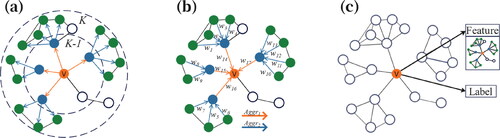
For clarity, consider Figure 4 as an illustrative example. First, we randomly sample neighbors in the $k$th and $k-1$th layers (as shown in Figure 4(a)), with a neighbor node sampling count of 4. Second, the collated information is progressively aggregated, transitioning from the external to the internal nodes (as illustrated in Figure 4(b)). Lastly, this aggregated intel serves as the input for the subsequent layer network, predicting the matching pattern of the ditch (as portrayed in Figure 4(c)).

Figure 4. Illustration of the process of neighbor sampling and aggregation: (a) sampling nodes from local neighbors; (b) aggregating feature information; (c) predicting the current state of the node.

3.1.2. TAGCN convolution operation

TAGConv represents the graph convolution operation within the TAGCN. More precisely, it is the multiplication of graph adjacency matrix polynomials. This operation is adept at extracting features from higher-order neighborhoods. Unlike traditional GCN convolution operations that rely on linear approximation, TAGCN convolution operation is exact. TAGConv employs a range of filters with sizes from 1 to $K$ in order to avoid linear approximation, thereby facilitating the capture of information from more distant nodes. For instance, when $K=3$ TAGConv uses 3rd-order filters to extract features from local regions with perception fields ranging in size from 1 to 3. The resulting output feature $y_f^{[\mathcal{l}]}$ is a weighted aggregate of convolution results from filters of varied sizes. (3) $$y_f^{\left[\mathcal{l}\right]}(i)=\sum _{k=1}^K\sum _{c=1}^{C_{\mathcal{l}}}\sum _j^{}{g}_{c,f,k}^{\left[\mathcal{l}\right]}w(p_{j,i}^k)x_c^{\left[\mathcal{l}\right]}(j)+b_f{1}_{N_{\mathcal{l}}}$$(3)

In the formula, $C_{\mathcal{l}}{}_{}^{}$ denotes the number of features in the $\mathcal{l}$th hidden layer, $j$ represents the set of paths that are $k$ distances away from vertex $i,$ $w(p_{j,i}^k)$ represents the cumulative weights of all paths at distance $k,$ $x_c^{[\mathcal{l}]}$ represents the input data of the $c$th feature across all nodes, $1_{N_{\mathcal{l}}}$ is a vector corresponding to a singular node in the graph with a dimension of 1, and $b_f$ is the bias term.

3.1.3. Model architecture for matching pattern identification

In view of the advantages of SAGEConv in processing large-scale graph structures, and the consistency of its sampling ideas with the cartographic generalization of ditch data, this model has high applicability to ditch data processing. In addition, compared with the traditional GCN model that only retains the first-order Chebyshev polynomial, TAGConv can obtain information from farther nodes, so it is more suitable for matching pattern identification in ditches. Given these considerations, we formulated a GNN model comprising 3 SAGEConv layers and 1 TAGConv layer, specifically tailored for ditch data pattern identification. The model’s structure is depicted in Figure 5.

Figure 5. Graph classification model utilizing GraphSAGE and TAGCN. This model comprises four convolutional layers: three SAGEConv layers and one TAGConv layer.

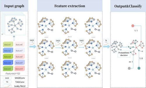
The matching pattern classification model is segmented into an input module, a feature extraction module and an output module. The model’s input consists of the graph’s structure and node labels. Within the feature extraction module, there are three SAGEConv layers and a singular TAGConv layer. The output module interprets the results from the feature extraction module and produces a node classification probability distribution. In the feature extraction component, the Leaky Rectified Linear Unit (LeakyReLU) is employed as the nonlinear activation function, mitigating the gradient vanishing issue inherent in ReLU by setting the negative_slope parameter to 0.01. In the concluding output module, the Softmax function is utilized to transition node features into class probabilities, yielding the final node classifications, indicative of the ditch’s matching pattern.

3.2. Performance evaluation methods

To evaluate the performance of the proposed method in this paper, we incorporated four prevalent metrics: Acc, P, recall (R) and F1 score (F1). Their respective computational formulas are as follows: (4) $$\mathit{Acc}=\frac{T\mathrm{P}+TN}{TP+TN+FP+FN}$$(4) (5) $$P=\frac{TP}{TP+FP}$$(5) (6) $$R=\frac{TP}{TP+FN}$$(6) (7) $$F1=2*\frac{P*R}{P+R}$$(7)

In the formulas above, TP denotes the count of samples predicted as category A that truly belong to category A, and $TN$ represents the count of samples predicted not to be in category A and are indeed outside of category A;$FP$ represents the samples predicted as category A but are not actually in that category and $FN$ represents the samples not predicted as category A but are genuinely in category A. Category A can correspond to one of the 1:0, 1:1 or M:1 matching patterns.

4. Experimental results and analysis

In order to evaluate the performance of the proposed model in identification of ditch matching patterns, multiple sets of experiments are designed from the following aspects to verify.

1. The performance of the model in the identification of ditch matching patterns (Section 4.1).

2. The impact of parameter settings on model performance (Section 4.2).

3. The impact of feature engineering on model performance (Section 4.3).

4. The advantages of the proposed model compared to other methods (Section 4.4).

4.1. Classification performance

4.1.1. Convergence process

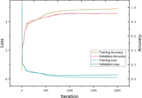
In this research, we employed a 4-layer network structure, comprising 3 SAGEConv layers and 1 TAGConv layer. The model’s input layer features 10 dimensions, and each convolutional layer contains 128 convolutional kernels. The TAGConv possesses 128 input dimensions and 3 output dimensions. A learning rate of 0.001 is set, and the LeakyReLU activation function is applied across all layers. Following 2000 iterations, the dropout is 0.3, the L2 regularization weight is 5e-4, the model effectively converged, registering a decline in the loss value to 0.04 and achieving an Acc of 90% on the validation set.

With the increase of the number of iterations, the loss values of the training set and the validation set tend to be stable, and the Acc of the training set and the validation set reach 0.983 and 0.919, respectively (Figure 6). The findings indicate that in the initial 500 iterations, both the training and validation accuracies saw a sharp ascent, paralleled by a swift reduction in their respective losses. From 500 to 1500 iterations, the rates of decline for the training and validation losses decelerated, recording reductions of 0.19 and 0.06, respectively, while the method’s Acc rose by 0.06. Beyond 1500 iterations, the losses for both training and validation began to stabilize, oscillating between 0.06 and 0.2, and the model’s Acc also demonstrated stability. All training metrics depicted a consistent fitting trajectory. To counteract potential overfitting, subsequent experiments determined that 2000 iterations represented the optimal selection.

Figure 6. Variations in training loss, validation loss, training accuracy and validation accuracy.

4.1.2. Overall evaluation

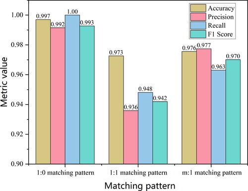
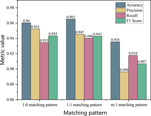
The method of matching pattern identification leveraging both SAGEConv and TAGConv has demonstrated its ability to adeptly discern various matching patterns, thereby enhancing the matching rate between multi-scale data. To substantiate the P and universality of this approach, we made predictions for each sample within the test set, subsequently evaluating the results rooted in these predictions. The Acc, P, R and F1 values of each matching pattern were calculated, and the overall Acc of the test set reached 0.973 (Figure 7). Notably, the majority of the ditch matching patterns have been precisely identified, with the 1:0 matching pattern showcasing an impeccable Acc rate of 100%. This high Acc can likely be attributed to the fact that during the multi-scale data transition, the ditch data exhibiting a 1:0 matching pattern solely underwent a deletion process, a modification effortlessly discernible by a GNN.

Figure 7. Evaluation of identification results for each matching pattern type.

4.1.3. Prediction results

The matching pattern prediction results of the test set are shown in Figure 8, where the gray line depict the ditch data from the training and validation sets, while colored lines illustrate the test set ditch data. Predictions for the matching patterns are labeled, and ditches encapsulated by red dashed rectangles indicate misclassification. From these predictions (Table 2), it’s evident that ditches with 1:1 and m:1 matching patterns were primarily misclassified. Conversely, those with a 0:1 matching pattern remained accurately classified. Specifically, ditches having a 1:1 matching pattern tend to be mislabeled as m:1, and vice versa.

Figure 8. Results of matching pattern identification in the test set.

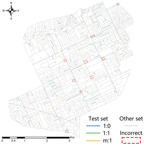
Table 2. Comparison of real and predicted matching patterns for selected ditch data.

Id	2845	2998	3036	3135	418	1265	1592	3077	3086
Real matching patterns	M:1	M:1	M:1	M:1	1:1	1:1	1:1	1:1	1:1
Predicted matching patterns	1:1	1:1	1:1	1:1	M:1	0:1	M:1	M:1	M:1

Considering geometric features, ditches at the extremes of the length spectrum (very long or very short) are typically classified correctly. Those misclassified generally fall within a length range of 60 − 260 m, highlighting the method’s reliance on geometric details. From a semantic standpoint, classification of ditches with Levels 1 and 2 poses challenges, while those at Level 3 are consistently accurate. This underscores the method’s recognition of the significance of ditch gradations. Regarding topological traits, ditches with elevated Adjaloop values often face misidentification. Essentially, nodes with a higher count of connecting edges in the ditch network duality graph lean towards misclassification. This intricacy closely ties with the sampling and aggregation processes of the network model presented in this paper. Consequently, enhancing the graph convolutional layer to efficiently learn from nodes with numerous connecting edges emerges as a pivotal avenue for refining classification Acc. Contextually, the MaxLength attribute for misclassified ditches is considerably large. However, its correlation with intrinsic factors like Sbet, Sconnect and Density is relatively tenuous, suggesting potential avenues for the method’s refinement in capturing ditch context features.

4.1.4. Extensibility of the model

In order to verify that the proposed model has good matching pattern classification performance for artificial ditches in different geographical regions, we added related experiments. The experimental area included artificial ditches in the Leeuwarden area of the Netherlands; there was a significant morphological difference between the artificial ditch in this area and the ditch data in the previous experiment (Figure 9), which was mainly manifested in the lack of obvious characteristics, such as parallel and right ditch angles. After preprocessing the data, we divided the entire ditch network into segments at the ditch intersection and level transition points, obtaining 3023 1:10,000 scale ditch segments and 1268 1:25,000 scale ditch segments. Among them, there are 1069 data with a matching pattern of 1:0, 922 data with a matching pattern of 1:1 and 1032 data with a matching pattern of m:1. At the same time, we divided the dataset into a training set, a validation set, and a test set according to the ratio of 6:2:2. We constructed this data into a graph structure and used it as a data input to evaluate the generalization performance of the model.

Figure 9. Data validation for scalability. (a) 1:10,000 ditch data; (b) 1:25,000 ditch data.

After 2000 iterations, the overall Acc of the test set reached 0.931. To evaluate the performance of the model more comprehensively, we also calculated the Acc, P, R and F1 values for each matching pattern (Figure 10). Experimental results show that the model has good classification performance for simple matching patterns 1:0 and 1:1, but there is still room for improvement in the classification Acc of ditch matching for m:1 mode. Considering that different forms of ditch data have different feature distributions, the quality of the data is crucial to the model’s performance. In addition, for different forms of ditch data, the methods adopted in cartographic generalization will be different, so the feature engineering of building a matching pattern classification model also needs to be adjusted according to the specific situation to improve the generalization ability of the model.

Figure 10. The classification performance of the model for different matching patterns.

4.2. Model framework and parameter analysis

4.2.1. Model framework analysis

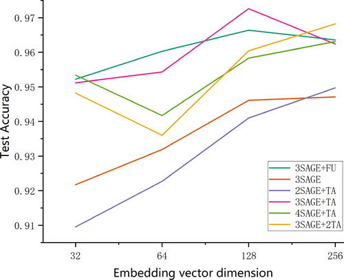
In To achieve an optimal network structure and embedding vector dimension, we conducted 24 experimental sets. Within these experiments, various network frameworks were explored including 3 SAGEConv layers with 1 fully connected layer, 3 SAGEConv layers alone, 2 SAGEConv layers combined with 1 TAGConv layer, 4 SAGEConv layers paired with 1 TAGConv layer and 3 SAGEConv layers coupled with 2 TAGConv layers.

These variations aimed to validate the efficacy of the TAGConv layer and to determine the most appropriate model depth. Concurrently, we adjusted the embedding vector dimensions through values of 32, 64, 128 and 256 to assess their influence on model performance and to identify the ideal pairing of embedding vector dimension with the network framework.

The GNN framework and embedding vector dimensions are related to model performance (Figure 11). Notably, the highest test Acc, 0.973, is achieved with a network framework comprising 3 SAGEConv layers and 1 TAGConv layer, using an embedding vector dimension of 128. Thus, we employed these parameters for this study. It is evident that the model network depth and the embedding vector dimension are not linearly related to test Acc. While enhancing the count of hidden layers and embedding vector dimensions augments information capacity, it can also precipitate gradient vanishing or explosion. With a model network depth of 4 layers, performance is commendable. The addition of a fully connected layer or a TAGConv layer enhances model efficacy, with the TAGConv layer proving more advantageous.

Figure 11. Influence of network framework and embedding vector dimension on accuracy.

4.2.2. Hyperparameters analysis

To delve deeper into the effects of various model hyperparameters on Acc, we executed experiments and conducted a quantitative analysis of the performance variations due to different hyperparameters in matching pattern identification. We zeroed in on the value of dropout, the activation function, the aggregation function in SAGEConv layers and the number of filter layers in TAGConv layers as our areas of interest. For the experiments, the values of dropout are 0.1, 0.3 and 0.5. The activation functions were chosen from the commonly used ReLU, ELU and LeakyReLU functions. The aggregation function in SAGEConv layers was determined among LSTM, max pooling, and average pooling functions and the filter layers were set to numbers 2, 3 and 4. The experimental results are shown in Figure 12.

Figure 12. Impact of different parameters on model performance.

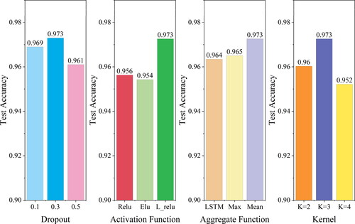
During of model training, adding a dropout layer can effectively constrain the generation of overfitting. Experimental results show that when dropout = 0.3, the classification Acc of the model on the test set reaches the highest. When dropout = 0.5, the performance of the model is not as good as that of the model at dropout = 0.1. This may be because excessive information is lost during training at dropout = 0.5, making the model unable to learn and understand patterns in the data effectively. From our examination of activation functions, we discerned that the choice of activation function markedly influences model effectiveness. Among them, the ELU function fared the poorest, while the LeakyReLU function emerged as the most effective. Assessing aggregation functions, the LSTM, Max and Mean functions all registered commendable test Acc. Notably, the mean function stood out, offering not only reduced computational complexity but also the pinnacle of test Acc. Evaluating the number of filter layers revealed that a setting of 3 layers yielded the apex of test Acc. Consequently, for this study, we set the dropout to 0.3, opted for the LeakyReLU function as our activation function, chose Mean for the aggregation function in SAGEConv layers, and designated the filter layer count to be 3.

4.3. Analysis of node features

4.3.1. Effect of different node features on identification performance

While keeping other hyperparameters constant, we assessed the influence of node features on model Acc. For this purpose, we set up the following experiments: First, we analyzed the Acc of the model by taking one indicators or all but one of the indicators as input variables. As per Figure 13(a), with all 8 node features as input, the model’s Acc peaked at 97.3%. A reduction in Acc below 97.3% was observed if any node feature was excluded, suggesting that each feature contributes to the classification of matching patterns. Notably, the omission of the Density and MaxLength features resulted in a marked decrease in Acc. This underscores the significance of maintaining density comparison and overall framework morphology across different scales of ditch data. Thus, during data matching, emphasis should be placed on these features. When only one feature indicator was entered, we found that the MaxLength feature of the ditch had the greatest impact on the model, followed by the Sbet feature of the ditch, and the topological features of the ditch (AdjaLoop and AdjaLake) had less impact. The experimental results further revealed the importance of MaxLength in ditch matching pattern identification. This is closely related to the fact that the overall structure of the ditch network is considered first in the process of ditch cartographic generalization, because the ditch with a larger MaxLength plays a key role in maintaining the overall structure of the ditch network.

Figure 13. Influence of node features on model performance.

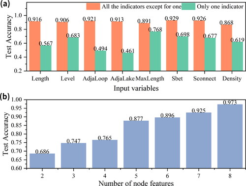
Second, the model was trained with varying numbers of node features to determine its classification performance. In the experiment that delved into the correlation between the quantity of node features and the model’s classification performance, the ensuing results were noted: When only the geometric and semantic node features (Length and Level) were considered, the model’s Acc stood at 68.6%. With the inclusion of topological features (AdjaLoop and AdjaLake), Acc rose to 76.2%. Finally, introducing contextual features (MaxLength, Sbet, Sconnect and Density) elevated the Acc to 97.3%. Through varying node feature quantities, we discerned that the addition of AdjaLoop, MaxLength and Density attributes considerably enhanced the model’s Acc.

4.3.2. Effect of a single feature on matching pattern identification performance

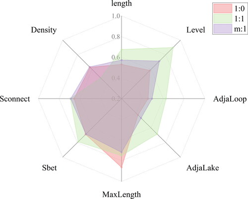
We further investigated the extent to which the input of only one node feature affects the different matching models (Figure 14). We used different node features to evaluate the performance of each feature in different ditch-matching pattern identification experiments. The results show that the model using only MaxLength as a feature has higher Acc when recognizing 1:0 matching patterns. This is mainly due to the fact that ditches with a smaller MaxLength are easily removed when the scale is changed. When it comes to identifying 1:1 matching patterns, the model Acc using only Level features is higher. This is mainly due to the fact that in spatial databases of different scales, the higher-level ditches are preserved. When identifying the m:1 matching pattern, the Acc of the model using only the MaxLength and Level features is high, reaching 0.7. This may be because the identification of the m:1 matching pattern is based on the characteristics of the first two matching patterns. Therefore, both of these features play a key role in identifying this matching pattern.

Figure 14. Effect of a single indicator on matching pattern identification performance.

4.4. Contrast experiment

4.4.1. Comparative analysis of model performance

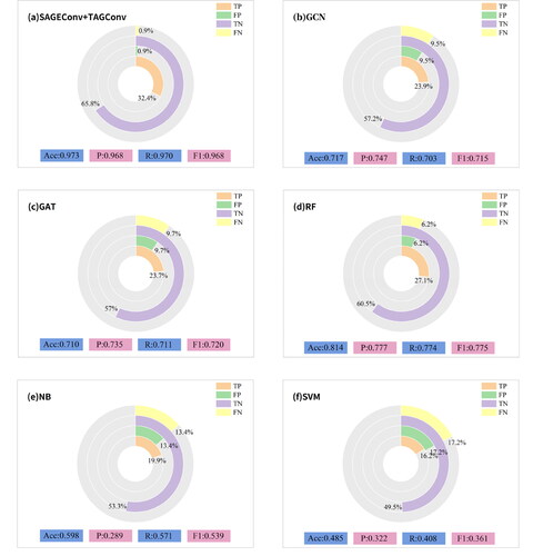
To discern the distinctions between the model method presented in this paper and other classification methods, we conducted a comparison with machine learning techniques including GCN, Graph Attention Network (GAT), Random Forest (RF), Naive Bayes (NB) and Support Vector Machine (SVM). The identical dataset was employed in the comparative experiment to confirm that our method can adeptly capture the deep features of 1:10,000 ditch data, demonstrating robust classification capabilities. In the GCN technique, a network structure incorporating three GCNConv layers and a singular fully connected layer was utilized, maintaining a maximum iteration count of 2000 and retaining other hyperparameters consistent with this paper’s model. The parameters for the GAT technique were equivalently set. In the RF method, set the number of decision trees is set to 200. In the NB method, the classifier selects the Gaussian model, and the smoothing variable is set to 1e-9. For the SVM approach, the kernel function was designated as the linear kernel function with a penalty coefficient of 0.8. The results of this comparative analysis can be viewed in Figure 15.

Figure 15. Comparison of accuracy results among various machine learning methods.

Our method employs the aggregation function within the SAGEConv layer to distill ditch segment feature details, comprehensively grasping the local context traits of ditch segments. Subsequently, the filtering mechanism in the TAGConv layer is harnessed to proficiently finalize the classification endeavor.

The GAT method allocates weights to first-order neighboring nodes via an attention mechanism and amalgamates adjacent node data contingent upon edge weight correlations. Yet, this mechanism might exhibit varied sensitivities to distinct features, potentially yielding unjustified weights, which could in turn impinge on overall efficacy. The proposed GNN model in this article aggregates data from neighboring nodes using an aggregation function, eschewing the assignment of weights to edges. The model capitalizes on the complementary nature of aggregation functions and filters to access multi-order neighborhood data, thus endowing the model with the capability to assimilate more characteristics of neighboring nodes. According to the experimental results of traditional machine learning, we can observe that the RF method performs well in processing high-dimensional data (data with many features) and has good generalization ability. However, the NB and the SVM methods performed relatively poorly. The main reason for this is that the naive Bayesian approach faces challenges when dealing with high-dimensional data, and the results are not satisfactory. At the same time, the performance of SVM is significantly reduced in the face of large-scale data and multi-classification problems. In summary, traditional machine learning methods such as SVMs do not perform well in this regard. These methods have obvious limitations and difficulties in the key steps, such as deep mining of network information and multi-classification using feature information.

Both the methodology proposed in this paper and the GCN approach embrace graph deep learning strategies. They fulfill the objective of matching pattern identification for 1:10,000 ditch data via data-driven supervised learning techniques. When juxtaposed with traditional metric-based regulations, data-driven strategies exhibit enhanced adaptability in feature selection and can manifest a certain generalization proficiency across data of diverse scales. Moreover, in comparison to the GCN technique, our method can discern data from non-first-order neighbors that are proximally situated and finalize the iterative data transmission process through sampling and aggregation procedures.

4.4.2. Significance test

In order to further illustrate the difference between this model method and other classification methods, we conducted 30 independent replicate experiments on GCN, GAT, RF, NB, SVM and the models mentioned in this article. At the same time, we evaluated the significance of the classification Acc of each comparison method and the method in this study (Table 3) to more accurately illustrate the superiority of the proposed method in classification Acc. In this article, the statistical method of paired t-test is used to analyze the difference between paired data, and if the p value is less than 0.05, it means that based on these 30 experiments, we can consider that the classification Acc of the comparison method is lower than that of the method described in this paper. The t-value is the ratio of the sample regression coefficient to the standard deviation, and the larger the t-value, the more statistically significant the result. During the experiment, for models that were set with random seeds, we changed the random seeds synchronously at the time of each experiment. According to the experimental results, we found that the p value of each group of the t-test was less than 0.05, and the absolute value of t-value exceeded the statistically critical value, indicating that the classification method proposed in this article outperformed other comparison methods in terms of Acc. The t-value of the GAT group was small, which may be due to the fact that the classification Acc of GAT was easily affected by random seed size, resulting in its unstable classification Acc.

Table 3. t-Test results of the classification accuracy of the method compared with the method in this paper.

	GCN	GAT	RF	NB	SVM
t-Value	66.79	21.79	78.42	232.16	303.33
P Value	2.54E-22	3.66E-14	1.67E-23	1.65E-31	1.76E-33

5. Discussion

Experimental results show that the proposed method is superior to other models in terms of Acc. First, this is the first time that GCNs are introduced into the matching pattern recognition of ditches, which enriches the research methods in this field and achieves significant classification effects. This fully proves that the method can effectively explore the reasons for the diversification of multi-scale ditch matching patterns, and can use this potential knowledge for classification. In addition, for m:1 type ditches, the method also achieves good identification results, which lays a solid foundation for the subsequent identification of n:m type ditches.

The GraphSAGE model has significant advantages in large-scale graph data processing, and it can obtain node features more comprehensively through sampling and aggregation technology based on neighborhood information, and then captures the relationship and influence between ditch segments. In addition, setting the last layer of the network model to the fully connected layer or the TAGConv layer can improve the performance of the model, among which the TAGConv layer performs particularly well because the TAGConv layer has a stronger ability to learn the information of farther nodes. When applied to different regions and different forms of ditch network data, different embedding vector dimensions, aggregation functions and loss functions can be flexibly adjusted and customized to learn the general representation of nodes in the graph structure.

In terms of feature setting, we draw on the feature setting of relevant elements in cartographic generalization, and comprehensively consider the characteristics of geometry, topology and context. Experimental results show that the lack of any node feature will lead to the decrease of model Acc. In particular, when the two features of Density and MaxLength are missing, the Acc of the model decreases greatly, which indicates that these two features have an important influence in feature engineering. This also meets the requirements of multi-scale ditch data production, that is, different scale ditch data need to maintain the original density comparison and overall structure.

Compared to GCN methods, the method proposed in this article considers more fully the information of key multi-order neighbors and also takes into account nodes that are close in real-world distance but not directly adjacent. Compared with GAT, this method does not need to assign weights to first-order neighbor nodes, and has better compatibility when learning neighbor nodes, which makes the classification performance better. In addition, compared to SVM methods, this method can more effectively mine deeper layers of information and exhibit certain generalization performance on different datasets. Therefore, this method can better obtain the matching pattern of 1:10,000 ditch data corresponding to 1:25,000 data.

6. Conclusions

In this article, we propose a GNN model incorporating both SAGEConv and TAGConv layers. The objective of this model is to identify the matching pattern of 1:10,000 ditch data during the matching process between 1:10,000 and 1:25,000 ditch data scales. This methodology treats segments of ditch networks as fundamental units, extracting geometric, semantic, topological and contextual features of ditch sections to represent graph node attributes. The topological relationships between these sections are articulated through graph structures. Input data comprises labeled graphs with node attributes, facilitating learning based on case scenarios. Through supervised training, sampling and aggregation methods yield richer, more abstract feature information. TAGConv is subsequently employed to map ‘feature representations’ into label spaces, culminating in the classification of ditch matching patterns. This approach alleviates the challenges associated with matching 1:10,000 ditch data to other scales, thereby enhancing matching rate and Acc. Importantly, our method pioneers the transformation of the multi-scale data matching challenge into a pattern identification issue. By harnessing the capabilities of GNNs in vector data feature learning, we can delve deeper into the intricacies of the ditch network, furnishing attribute references for ditch data matching. We tested this method on 1:10,000 scale ditch data from the Overijssel region in the Netherlands, employing a classification model with three SAGEConv layers and one TAGConv layer. Using a 1:25,000 scale map for reference, we annotated its matching patterns. The model’s classification Acc peaked at 97.3%. This rate surpasses other GNN methods by 25.6 − 26.3% and exceeds traditional machine learning techniques by 33%.

Our approach is grounded in the underlying cause of multi-scale data discrepancies: cartographic generalization. Given the relative simplicity of cartographic generalization for ditch data, future research will shift focus towards identifying matching patterns for more intricate geographic entities like roads and settlements. With these enhancements, our aim is to deepen our grasp of cartographic generalization, harnessing it more effectively to offer precise and efficient solutions for complex geographic entity matching issues.

Author contributors

Zhekun Huang conceived the original idea for this study, implemented the code, contributed to writing and completed the first draft. Haizhong Qian supervised the research and edited and reviewed the manuscript. Other authors estimated the proposed approach, evaluated its applicability and processed the data.

Disclosure statement

No potential conflict of interest was reported by the authors.

Data availability statement

Data, models or code generated or used during the study are available from the corresponding author upon request.

Additional information

Funding

This work was supported by the Natural Science Foundation for Distinguished Young Scholars of Henan Province (212300410014) and the National Natural Science Foundation of China (42271463, 42101453 and 42371461).

References

- Ai T. 2021. Some thoughts on empowering map making with deep learning. Acta Geod Cartogr Sin. 50(9):1170–1182.
- Chehreghan A, Ali Abbaspour R. 2017. A new descriptor for improving geometric-based matching of linear objects on multi-scale datasets. GIScience Remote Sens. 54(6):836–861. doi:10.1080/15481603.2017.1338390.
- Chehreghan A, Ali Abbaspour R. 2018. A geometric-based approach for road matching on multi-scale datasets using a genetic algorithm. Cartogr Geogr Inf Sci. 45(3):255–269. doi:10.1080/15230406.2017.1324823.
- Chen J, Qian H, Wang X, He H, Hu H. 2016. Dynamic simplification method to improve the matching rate of line features. Acta Geod Cartogr Sin. 45(4):486–493.
- Duan P, Qian H, He H, Liu C, Xie L. 2019. A lake selection method based on dynamic multi-scale clustering. Geom Inf Sci Wuhan Univ. 44(10):1567–1574.
- Duan P, Qian H, He H, Xie L, Luo D. 2020. A line simplification method based on support vector machine. Geom Inf Sci Wuhan Univ. 45(5):744–752.
- Fu Z, Yang Y, Gao X, Zhao X, Fan L. 2016. A multi-feature matching optimization algorithm for road networks. Acta Geod Cartogr Sin. 45(5):608–615.
- Gao X, Yan H, Lu X. 2022. A semantic similarity calculation method for multi-scale map spatial residential areas. Acta Geod Cartogr Sin. 51(1):95–103.
- Guo W, Liu H, Sun Q, Yu A, Ding Z. 2019. A multi-source contour matching method considering geometric feature similarity. Acta Geod Cartogr Sin. 48(5):643–653.
- Kim JO, Yu K, Heo J, Lee WH. 2010. A new method for matching objects in two different geospatial datasets based on the geographic context. Comput Geosci. 36(9):1115–1122. doi:10.1016/j.cageo.2010.04.003.
- Lei TL. 2021. Large scale geospatial data conflation: a feature matching framework based on optimization and divide-and-conquer. Comput Environ Urban Syst. 87:101618. doi:10.1016/j.compenvurbsys.2021.101618.
- Li L, Goodchild MF. 2011. An optimisation model for linear feature matching in geographical data conflation. Int J Image Data Fusion. 2(4):309–328. doi:10.1080/19479832.2011.577458.
- Liu C, Wu F, Gong X, Xing R, Du J. 2021a. A clustering method for natural surface clustering degree based on spatial knowledge mining. Acta Geod Cartogr Sin. 50(4):544–555.
- Liu C, Wu F, Gong X, Xing R, Du J. 2021b. Pattern recognition of complex distributed ditches. IJGI. 10(7):450. doi:10.3390/ijgi10070450.
- Liu L, Ding X, Zhu X, Fan L, Gong J. 2020. An iterative approach based on contextual information for matching multi‐scale polygonal object datasets. Trans GIS. 24(4):1047–1072. doi:10.1111/tgis.12625.
- Sandro S, Massimo R, Matteo Z. 2011. Pattern recognition and typification of ditches. In: Ruas A, editor. Advances in cartography and GIScience. Vol 1. Berlin, Heidelberg, Germany: Springer Berlin Heidelberg; p. 425–437.
- Tong X, Liang D, Jin Y. 2014. A linear road object matching method for conflation based on optimization and logistic regression. Int J Geogr Inf Sci. 28(4):824–846. doi:10.1080/13658816.2013.876501.
- Wang H, Liu Y, Li S, Liang B, He Z. 2023. A GNSS high sampling rate path incremental map matching method. Acta Geod Cartogr Sin. 52(2):329–340.
- Wang M, Ai T, Yan X, Xiao Y. 2020. Recognition of road orthogonal grid pattern by graph convolutional network model. Geom Inf Sci Wuhan Univ. 45(12):1960–1969.
- Wang W, Yan H, Lu X, He Y, Liu T, Li W, Li P, Xu F. 2023. Drainage pattern recognition method considering local basin shape based on graph neural network. Int J Digit Earth. 16(1):593–619. doi:10.1080/17538947.2023.2172224.
- Wu H, Xu S, Huang S, Wang J, Yang X, Liu C, Zhang Y. 2022. Optimal road matching by relaxation to min-cost network flow. Int J Appl Earth Obs Geoinf. 114:103057. doi:10.1016/j.jag.2022.103057.
- Yang M, Jiang C, Yan X, Ai T, Cao M, Chen W. 2022. Detecting interchanges in road networks using a graph convolutional network approach. Int J Geogr Inf Sci. 36(6):1119–1139. doi:10.1080/13658816.2021.2024195.
- Yang M, Kong B, Dang R, Yan X. 2022. Classifying urban functional regions by integrating buildings and points-of-interest using a stacking ensemble method. Int J Appl Earth Obs Geoinf. 108:102753. doi:10.1016/j.jag.2022.102753.
- Yu W, Liu M. 2023. An iterative framework with active learning to match segments in road networks. Cartogr Geogr Inf Sci. 50(4):333–350. doi:10.1080/15230406.2023.2190935.
- Zhang J, Wang Y, Zhao W. 2018. An improved probabilistic relaxation method for matching multi-scale road networks. Int J Digit Earth. 11(6):635–655. doi:10.1080/17538947.2017.1341557.
- Zhang M, Meng L. 2007. An iterative road-matching approach for the integration of postal data. Comput Environ Urban Syst. 31(5):597–615. doi:10.1016/j.compenvurbsys.2007.08.008.
- Zhang WB, Ge Y, Leung Y, Zhou Y. 2021. A georeferenced graph model for geospatial data matching by optimising measures of similarity across multiple scales. Int J Geogr Inf Sci. 35(11):2339–2355. doi:10.1080/13658816.2020.1858301.
- Zhang X, Ai T, Stoter J, Zhao X. 2014. Data matching of building polygons at multiple map scales improved by contextual information and relaxation. ISPRS J Photogramm. 92:147–163. doi:10.1016/j.isprsjprs.2014.03.010.
- Zhang X, He X, Sun Y, Huang J, Zhang Z. 2022. Research status and prospects of multi-scale spatial data linkage update technology. Acta Geod Cartogr Sin. 51(7):1520–1535.
- Zheng J, Gao Z, Ma J, Shen J, Zhang K. 2021. Deep graph convolutional networks for accurate automatic road network selection. IJGI. 10(11):768. doi:10.3390/ijgi10110768.
- Zhong D. 2018. Research on line feature quality evaluation and multi-scale water system matching method. Wuhan, China: Wuhan University.