Detection of terrain feature points from digital elevation models using contour context

Abstract

Terrain feature points, such as peaks, pits, and saddles, represent the macro-structure of the landform. Conventional techniques for extracting these points from digital elevation models (DEMs) often grapple with issues of inaccuracy, omission and redundancy, largely due to the problematic necessity of setting threshold values. This paper proposes an innovative approach for the automatic detection of terrain feature points based on the topological relationships of contours and the inherent constraints of terrain shape characteristics. The study provides a robust mathematical model of terrain feature points and an effective algorithm for their extraction. Comparing with manually reference data, the accuracy metrics including completeness, correctness, and quality of our extracted results demonstrate a high level, significantly surpassing those obtained through existing algorithms. This proposed approach not only avoids the spurious feature points produced by the local window method, but also prevents the omission of valid points and the creation of redundant ones. Moreover, by utilizing the contour interval as its only variable, our approach eliminates the need for various threshold settings, streamlining the extraction process.

Keywords:

• Digital elevation model (DEM)
• terrain feature points
• contour topological relationship
• contour interval
• geomorphology

1. Introduction

One of the main tasks of geomorphology is to divide topographic surfaces into units or objects (Wilson 2018). The terrain feature points located at the transitions of topographic surfaces, such as peaks, pits and various saddles, are the most important morphological elements. These terrain feature points can describe the topographic structural characteristics and reveal topographic semantic information, and can also be taken as the basic variables in geoscience fields, such as hydrological analysis (Heckmann et al. 2015; Tavares et al. 2019), cartographic synthesis (Ai and Li 2010; Samsonov 2022), surface network construction (Wang and Yu 2009; Clarke and Romero 2017) and digital soil mapping (Florinsky 2016; Neyestani et al. 2021). Therefore, the objective analysis, description and expression of geomorphic morphological elements have long been a focus of geographers.

At present, the topographic features such as peaks, pits, and saddles are basically extracted from DEMs. Although DEMs are available in various data formats including regular grid models, irregular triangulated networks (TINs), contour lines, and point clouds etc. (Wilson 2018), the most common methods for peak, pit, and saddle extractions as well as terrain classification are using grid-based DEMs (Cheng et al. 2022). According to predefined rules and local moving windows, these topographic features can be classified and extracted from grid-based DEMs (Etzelmüller 2000; Pike 2000).

One of the earliest algorithms to automatically extract topographic feature points from DEMs was the eight-neighborhood method proposed by Peucker and Douglas (1975). In a 3 × 3 moving window of the DEM, the central grid cell is assigned to terrain feature point types according to its elevation difference from its eight surrounding cells, as well as the rules governing the changes in this difference. This method, noted for its simplicity and easy parallelization, has been adopted by many scholars (Etzelmüller 2000; Bolongaro-Crevenna et al. 2005). Dikau (2020) proposed a terrain classification scheme based on the combination of slope and curvature of the central unit in a local window. Takahashi et al. (1995) believed that the terrain feature points extracted using the eight-neighbor method should satisfy Euler’s theorem (N_Peak + N_Pit − N_Saddle = 2, where N_Peak, N_Pit and N_Saddle are the numbers of peaks, pits, and saddles respectively). And he proposed a local window triangulation method with the introduction of virtual pits or peaks to ensure that the extracted features meet Euler’s theorem. Schneider (2005) proposed a terrain feature point extraction method from DEMs by using a bilinear interpolation scheme, where the type of each grid cell was identified through the elevation of its four adjacent grid cells. Wood and Rana (2000) and Schneider and Wood (2004) developed a classification method based on quadric surfaces fitted by DEM grid neighborhoods, in which the category of each grid cell was determined by the types of quadric surfaces (elliptic, paraboloid and hyperboloid). Wood (1996) developed a multi-resolution terrain feature classification method based on quadratic surfaces. Weiss (2001) proposed a classification indicator called Topographic Position Index (TPI), which measured the relative height of one point relative to its surrounding area using two different window sizes on DEMs to perform the terrain classification. Jasiewicz and Stepinski (2013) proposed a promising pattern recognition approach called Geomorphons to automatically classify the terrain features including peaks, pits and saddles, which was based on the principles of local gradient and line-of-sight calculation.

Another approach to identify terrain feature points from DEMs is called stream network analysis or hydrological analysis method (Zhang et al. 2014; Li et al. 2022), which is usually achieved by Geographic Information System (GIS) software like ArcGIS (Zhang et al. 2011; ESRI, 2020). Based on a series of processes, the direction of streams can be calculated and watersheds, features points and feature lines can be extracted through the water accumulation simulation.

However, in the terrain analysis based on DEMs, the extraction of topographic features such as peaks, pits and saddles has always been faced with the following challenges. First, the inherent errors and uncertainties in DEM data limit the accuracy of feature detection (Anders et al. 2013; Zhou et al. 2019), resulting in many pseudo-terrain features in classification algorithms (Takahashi et al. 1995; Schneider and Wood 2004). Second, terrain types are the external manifestations of geological and geomorphological processes, as well as a comprehensive representation related to multiple geomorphological processes. The finiteness of terrain classification parameters and the comprehensiveness of geomorphological types also lead to the uncertainty of terrain feature extraction and classification (Schmidt and Allan 2004; Bolongaro-Crevenna et al. 2005). Third, existing terrain feature extraction methods are scale-dependent, involving factors such as DEM resolution (Arundel et al. 2018; Mokarram et al. 2018), the size of local window units (Wood 1996; MacMillan and Shary 2009), and various threshold sizes (Florinsky 2009; Zhao et al. 2014; Zhou et al. 2019; Hu et al. 2022).

To achieve a comprehensive, precise, and natural extraction of terrain features from DEMs, this study introduces an advanced method for the automatic identification of peaks, pits, and saddles. This approach is distinguished by its integration of the contextual information inherent in contour lines, enhancing the natural representation of the topography. The idea originates from the human cognition of contour topographic maps. That is, through the adjacent, nested, and hierarchical spatial topological relationships between contour lines, the concavity and convexity rules of contour lines, as well as the elevation values, people can reconstruct regional 3D topography (Imhof 1982), thereby achieving judgements on the overall structure and local morphology of the regional geomorphology (Cromley, 1991; Guilbert 2013), especially features like peaks, pits and saddles.

The main contributions of this paper include the following three aspects. (1) Mathematical models of terrain features including peaks, pits and saddles have been constructed by combining representing methods and geomorphological cognition patterns of contour topographic maps. (2) Based on grid DEMs, interpretation algorithms for peaks, pits and saddles have been proposed, which are also suitable for TINs, contour lines, and other forms of DEMs. (3) This paper presents a global method rather than a local window means for feature recognition, with the contour interval as its only variable when the resolution of DEM is fixed. And the influence laws of the contour interval on the quantity and location of key points have also been discussed through experiments.

The remainder of this article is organized as follows. Section 2 describes the development of a mathematical model and interpretation algorithm for terrain feature point extraction based on contour line features, such as peaks, pits and various saddles. Section 3 presents a systematic experimental analysis of the proposed method. Section 4 has a discussion between our method and the existing literature. Finally, Section 5 presents the concluding remarks.

2. Methodology

Based on the location features of terrain feature points, this section first provides an analysis of the basic features of contour lines near feature points, then describes the construction of a morphological mathematical model of feature points, and finally presents a novel interpretation algorithm for terrain feature points.

2.1. Mathematical model of terrain feature points based on contour topological relationships

2.1.1. Feature contour lines

Here, three types of contour lines are introduced, namely basic contour line, feature contour lines and self-intersecting contour line. (1) In topographic maps, the contour lines determined according to the basic contour interval are called the basic contour lines (Imhof 1982). (2) There are three contour lines in the vicinity of any point on the ground: one contour line passing through the point (the self-contour line), and the two contour lines that are closest to the point, namely, the contour lines above the point (the higher contour line) and below the point (the lower contour line). These three contour lines are termed the feature contour lines of the point. Since a point can also be seen as a degenerated line, the self-contour line on this point is termed a degraded contour line. (3) In addition to the above contours, there exists a special contour line, self-intersecting contour line, which are defined as two adjacent lines in the same plane with the same elevation share a point (such as a saddle point). Obviously, self-intersecting contour line is a special case of the self-contour line.

In the definitions above, the higher and lower contour lines are determined by the contour interval and the elevation at the focal point. Apart from the self-contour line, the higher and lower contour lines at a point are also basic contours. Obviously, there is one and only one self-intersecting contour line at a saddle, while there is a self-contour line at each peak and pit. Therefore, the topographic features of any point can be completely determined by the geometric features of its self-contour line and the topological relations between the feature contour lines.

As shown in Figure 1, the feature contour lines at a peak, pit and saddle have the following characteristics.

Figure 1. Spatial relationship between feature contour lines (H indicates elevation above the sea level. Since feature contour lines are related to point position, more details can be founded in text).

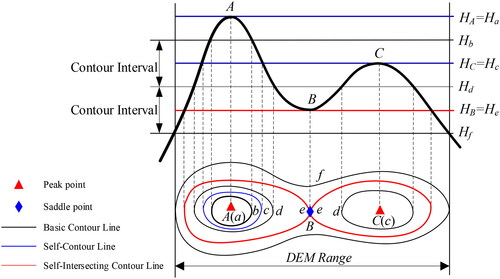
Peak: At a point, if only the lowest contour line containing itself and a self-contour line exist, this point is called the global peak (e.g. Point A in Figure 1; a is the self-contour line, b is the lower contour line). If all three feature contour lines exist simultaneously, and the lower contour line containing the point is separated from the higher contour line, then that point is deemed a local peak (e.g. Point C in Figure 1; c is the self-contour line, b is the higher contour line, d is the lower contour line).

Pit: A point at which only the self-contour line and the higher contour line exist is called the global pit. If all three feature contour lines exist simultaneously, and the higher contour line containing the point is separated from the lower contour line, then that point is deemed a local pit.

Saddle: If the self-intersecting contour line, the higher contour line and the lower contour line exist at the same point (e.g. Point B in Figure 1; e is the self-intersecting contour line, f is the lower contour line, d is the higher contour line), and the lower (higher) contour contains two separated higher (lower) contours with the same elevation, then this point is regarded as a saddle. If there is only one higher (lower) contour with the same elevation, the saddle at the basic contour interval is called an invisible saddle, as it cannot be displayed at the given contour interval.

2.1.2. Morphological mathematical model

Based on the above analysis, morphological mathematical models of the peak, pit and saddle can be defined as follows. Given a topographic surface $z=f(x,y),$ where its regional extent is $\Omega ,$ the contour interval is CI, and $Q(x_Q,y_Q,H_Q)$ is any point on $f(x,y),$ then the feature contour line Q can be defined as (1) $$\begin{array}{c}\mathit{\text{Self}}-\mathit{\text{contourline}}:C_S(Q)=H_Q=f(x_Q,y_Q)\\ h\mathit{\text{ighercontourline}}:C_H(Q)=\mathrm{\text{int}}(H_Q/\mathit{\text{CI}}+1)\times \mathit{\text{CI}}\\ l\mathit{\text{owercontourline}}:C_L(Q)=\mathrm{\text{int}}(H_Q/\mathit{\text{CI}})\times \mathit{\text{CI}}\end{array}\}$$(1) where $C_S(Q),C_H(Q),C_L(Q)$ refer not only to the contour lines themselves, but also to the area enclosed by the contour lines. This area is a closed region with the boundary $\Omega .$

If Q is a peak, it must be located in the area bounded by the lower contour line, and its elevation must be the same as that of the self-intersecting contour line. Q can be defined as (2) $$\begin{array}{l}Q\in C_L(Q)\wedge \{C_S(Q)=H_Q\vee (C_H(Q)\cap C_L(Q)=\varnothing \}\\ \underset{\mathit{\text{CI}}\to 0}{\mathrm{\text{lim}}}{C}_L(Q)=Q\end{array}\}$$(2)

If Q is a pit, it can be stated that (3) $$\begin{array}{l}Q\in C_H(Q)\wedge \{C_S(Q)=H_Q\vee (C_H(Q)\cap C_L(Q)=\varnothing \}\\ \underset{\mathit{\text{CI}}\to 0}{\mathrm{\text{lim}}}{C}_H(Q)=Q\end{array}\}$$(3)

If ${C^{\prime }}_L(Q),{C^{\prime }}_H(Q)$ are contour lines with the same elevation as $C_L(Q),C_H(Q),$ Q can be defined as a saddle with the following formula (4) $$\begin{array}{c}\mathit{\text{Positive }}\mathrm{\text{Re}}\mathit{\text{lief: }}{C}_S(Q)=H_Q\wedge \{C_H(Q)\cap {C^{\prime }}_H(Q)=\varnothing \}\subset C_L(Q)\\ \mathit{\text{Negative Relief}}:C_S(Q)=H_Q\wedge \{C_L(Q)\cap {C^{\prime }}_L(Q)=\varnothing \}\subset C_H(Q)\\ \underset{\mathit{\text{CI}}\to 0}{\mathrm{\text{lim}}}{C}_H(Q)=\underset{\mathit{\text{CI}}\to 0}{\mathrm{\text{lim}}}{C}_L(Q)=C_S(Q)\end{array}\}$$(4)

The second condition in (2)-(3) and the third condition in (4) express the multi-scale characteristic of Q, indicating that as the contour interval approaches zero, the lower contour line will shrink to a peak, pit or saddle.

2.2. Interpretation algorithm of terrain feature points from DEMs

According to the above analyses and definitions, the critical steps of topographic feature point extraction from DEMs are the acquisition of feature contours and the analysis of their topological relationships. As the topological relationships can be converted into relations between points and polygons, they will not be covered again here. The following passages focus on the calculation of the feature contour lines.

2.2.1. Contour calculation with arbitrary elevation

For an arbitrary point Q with elevation H_Q, the DEM can be converted into a binary image BI_DEM according to H_Q: (5) $$B{I}_{\mathit{\text{DEM}}}=\{\begin{array}{c}1\mathit{\text{DEM}}(i,j)\ge H_Q\hfill \\ 0\mathit{\text{DEM}}(i,j)<H_Q\hfill \end{array}$$(5)

On BI_DEM, a series of areas with elevations higher than H_Q form a connected region, and the boundary of this connected region forms the contour line across point Q, which can be identified by a boundary tracking algorithm (Figure 2). The feature contour lines can be calculated by replacing H_Q in Formula (5) with C_S(Q), C_H(Q) and C_L(Q).

Figure 2. Workflow for extracting contours from a DEM based on the image processing method (DEM resolution = 50 m; H_Q = 2310; red triangle signifies the location of point Q). (a) Binary image; (b) boundary of the connected region; (c) vectorized contour lines.

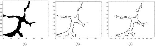
Compared with the conventional contour tracking algorithm, this method based on image processing avoids the problem of ambiguity. Furthermore, the extracted contours are self-closed within the DEM range, as the connected regions contain the DEM boundaries. In contrast, ensuring that contour lines are closed is always challenging in contour tree construction (Song et al. 2011). To obtain finer contour lines, DEM resampling can be used.

2.2.2. Identification of self-intersecting contour

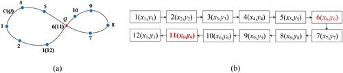
As mentioned above, a degraded self-intersecting contour line is just one point, so the contour linked list has just one entry, which records the position and elevation of this point. Meanwhile, non-degraded self-intersecting contour lines (e.g. contour lines through a saddle) share a common point that appears twice in a contour linked list. Therefore, intersections can be determined by whether there are repeated points in the linked list. Once the position of the common point in the linked list is determined, the decomposition of self-intersecting contours is completed.

Figure 3(a) and Figure 3(b), respectively, shows a contour C(Q) passing through arbitrary point Q and its linked list structure. The contour point (x₆, y₆) (Q) appears twice in the linked list, at position 6 (x₆, y₆) and position 11 (x₆, y₆). Thus, C(Q) can be determined as a self-intersecting contour. Taking positions 6 and 11 as breakpoints, C(Q) can be decomposed into two closed contours, {1, 2, 3, 4, 5, 6, 12 (1)} and {6, 7, 8, 9, 11(6)}.

Figure 3. Identification and decomposition of self-intersecting contour lines. (a) An example of a self-intersecting contour line (blue circles signify points with the same elevation; the red triangle signifies the point of self-intersection); (b) the linked list of the contour in (a).

2.2.3. Interpretation algorithm

Topographically, peaks only exist in positive terrain, pits only exist in negative terrain, and saddles appear in both positive and negative terrain. Therefore, the first task of this algorithm is to identify whether DEM grid cells are situated in positive or negative terrain. The proposed interpretation model for feature point extraction from DEM based on contour lines is shown in Algorithm 1.

Algorithm 1.

Interpretation algorithm for peak, pit and saddle extraction from DEM based on contour lines

Input: DEM, CI // CI: Contour interval

Output: Terrain Classification Matrix: DEM_C = 0 //1-Peak; 2-Saddle; 3-Pit; 0-Point on slope

1: Initialization DEM_C = 0

2: For Q ∈ DEM Do

3:  Q (Identification of positive or negative terrain← Divergence calculation

4:  Calculate C_S(Q), C_H(Q), C_L(Q)←Formula (1);

5:  If Q is in positive terrain //Peak area

6:   Get binary images of C_S(Q), C_H(Q), C_L(Q): BI_S(Q), BI_H(Q), BI_L(Q)← Formula (5);

7:   Boundaries of the connected domain of binary images form the linked lists of feature contours: C_S, C_H, C_L;

8:   Contours where Q is: C_H (Q), C_L (Q); // There are multiple lines with the same height, and it is necessary to confirm which one contains Q;

9:   If Length (C_H(Q)) = 0 & Length (C_L(Q)) > 1

10:    DEM_C (Q) = 1; //Global peak

11:   Else If Length (C_H(Q)) >0 & (C_L(Q) ∩ C_H(Q) = Ø)

12:    DEM_C(Q) = 1; //Local peak

13:   Else If Length (C_S(Q)) > 0 & (C_H(Q) ∩ C′_H(Q)=Ø) ⸦ C_L(Q)

14:    If max(P)∈(C_H(Q) ˅ C′_H(Q) & H_P<C_H(Q) & H_P > C_L(Q)

15:     DEM_C(Q) = 0; //Non-visible saddle with the contour interval CI

16:    Else

17:     DEM_C(Q) = 2; //Saddle in positive terrain

18:    End If

19:   End If

20:  Else Q is in negative terrain //Pit area

21:   Get binary images of C_S(Q), C_H(Q), C_L(Q): BI_S(Q), BI_H(Q), BI_L(Q)← “>” in Formula (5) → “<”

22:   Boundaries of the connected domain of binary images form the linked lists of feature contours: C_S, C_H, C_L;

23:   Contours where Q is: C_H (Q), C_L (Q); // There are multiple lines with the same height, and it is necessary to confirm which one contains Q;

24:   If Length (C_L(Q)) = 0 & Length (C_H(Q)) > 1

25:    DEM_C(Q) = 3; // Global pit

26:   Else If Length (C_L(Q)) >0 & (C_L(Q) ∩ C_H(Q) = Ø)

27:    DEM_C (Q) = 1; //Local pit

28:   Else If Length (C_S(Q)) > 0 & (C_L(Q) ∩ C′_L(Q) = Ø) ⸦ C_H(Q))

29:    If min(P) ∈ (C_L(Q) ˅ C′_L(Q)) & H_P > C_L(Q) & H_P < C_H(Q)

30:     DEM_C (Q) = 0; //Non-visible saddle with the contour interval CI

31:    Else

32:     DEM_C (Q) = 2; //Saddle in negative terrain

33:    End If

34:   End If

35:  End If

3. Experimental analysis

3.1. Dataset description

Considering that the number and location of feature points need to be analyzed statistically, and in order to avoid the influence of DEM errors on the analysis results, high-precision DEM data is selected. The original DEMs are derived by digitizing contour maps (Habib 2021). First, a large-scale contour map is scanned and digitized by AutoCAD to acquire contour lines with a spacing of 10 m. Second, the CAD mapping is imported into ESRI ArcGIS 10.2 as a feature class to generate DEMs using the interpolation technique ANUDEM with a resolution of 0.25 m. Finally, each 0.25 m DEM is bilinearly interpolated into a DEM with a resolution of 10 m. More details of the DEM dataset can be found in Habib (2021).

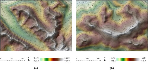
The experimental data of this study include a mountainous DEM and a hilly DEM with resolutions of 10 m (Figure 4). The DEM of the mountainous area covers 2.73 km², with a maximum elevation of 996.490 m and a minimum elevation of 671.076 m. The DEM of the hilly area is 2.77 km², with a maximum elevation of 623.634 m and a minimum elevation of 321.413 m. The topographies of the experimental areas have large relief, and peaks of various heights are clearly distributed across them.

Figure 4. Terrain surfaces of the test sites (Habib 2021). (a) Mountainous area; (b) hilly area.

In order to verify the effectiveness of the proposed method, we choose the manual extraction features from contour lines derived from DEMs as the reference data (Rutzinger et al. 2012; Zhou et al. 2018; Zhou et al.2019; Huang et al. 2020). To further ensure the objectivity of the manually extracted features, contour lines are overlayed on the corresponding hill-shading maps to assist the location interpretation of the terrain features. And the average value of multiple interpretation results is taken as the final reference data.

3.2. Overall results

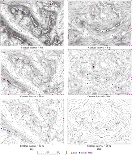
Figure 5 shows the results of topographic feature point extracted at contour intervals of 5-meter, 10-meter and 20-meter in the mountainous DEM and hilly DEM with 10-meter resolution. As can be seen from Figure 5, all peaks, pits and saddles except on the DEM boundary are correctly extracted by our approach. The extracted results are consistent with the manual extraction results (For clarity, the manual extraction results are not marked in Figure 5, but a part of them are shown in Figures 10 and 11), without any pseudo-topographic features or redundant topographic feature points.

Figure 5. Results of feature point extraction with different contour intervals (DEM resolution is 10 m). (a) Mountainous area; (b) hilly area.

In order to make a quantitative assessment between the peaks, pits and saddles extracted by the proposed method and those extracted manually from topographic maps, three accuracy metrics have been introduced, which are completeness, correctness and quality respectively (Rutzinger et al. 2012). Their calculation formulas are shown in the following Equation (6)(6) $$\begin{array}{c}\mathit{\text{Completeness}}=\frac{\mathit{\text{TP}}}{\mathit{\text{TP}}+\mathit{\text{FN}}}\times 100\%\\ \mathit{\text{Correctness}}=\frac{\mathit{\text{TP}}}{\mathit{\text{TP}}+\mathit{\text{FP}}}\times 100\%\\ \mathit{\text{Quality}}=\frac{\mathit{\text{TP}}}{\mathit{\text{TP}}+\mathit{\text{FP}}+\mathit{\text{FN}}}\times 100\%\end{array}\}$$(6) , where TP denotes the point number of true positive (correct extract), FN is the point number of false negative (incorrect extract, including redundant points) and FP is the point number of false positive (omissive extract). Therefore, for each extracted feature point, statistical parameters including the numbers of correct points, false points, redundant points and omissive points should be counted. (6) $$\begin{array}{c}\mathit{\text{Completeness}}=\frac{\mathit{\text{TP}}}{\mathit{\text{TP}}+\mathit{\text{FN}}}\times 100\%\\ \mathit{\text{Correctness}}=\frac{\mathit{\text{TP}}}{\mathit{\text{TP}}+\mathit{\text{FP}}}\times 100\%\\ \mathit{\text{Quality}}=\frac{\mathit{\text{TP}}}{\mathit{\text{TP}}+\mathit{\text{FP}}+\mathit{\text{FN}}}\times 100\%\end{array}\}$$(6)

The overall quantitative evaluation results of the mountainous data set and hilly data set are shown in Table 1 and Table 2, respectively. As can be seen from Tables 1 and 2, the proposed method can achieve high correctness and completeness in both two data sets, with three accuracy metrics almost up to 100%. This mainly results from the fact that a set of contour lines, not an individual line itself, depict the major features of a landscape and retain its intrinsic character (Guilbert 2013). Contour lines are governed by clear rules and follow explicit spatial relationships for terrain expression, so that pseudo-topographic feature points are effectively avoided due to the mutual relationship between contour lines and the topological relation between feature points and contour lines.

Table 1. Accuracy comparison results in mountainous area.

Contour interval (m)	Feature points	Manual method	Proposed method	Accuracy metrics
5	Peaks	23	23/0/0/0	(100%, 100%, 100%)
	Saddles	25	24/0/0/1	(100%, 96%, 100%)
	Pits	2	2/0/0/0	(100%, 100%, 100%)
10	Peaks	14	14/0/0/0	(100%, 100%, 100%)
	Saddles	15	15/0/0/0	(100%, 100%, 100%)
	Pits	2	2/0/0/0	(100%, 100%, 100%)
20	Peaks	10	10/0/0/0	(100%, 100%, 100%)
	Saddles	19	19/0/0/0	(100%, 100%, 100%)
	Pits	2	2/0/0/0	(100%, 100%, 100%)

Digit in A/B/C/D represent the number of totals, false, redundant, and omissive feature points respectively in the proposed method column. Digit in (A, B, C) denotes the completeness, correctness and quality in the accuracy column.

Table 2. Accuracy comparison results in hilly area.

Contour interval (m)	Feature points	Manual method	Proposed method	Accuracy metrics
5	Peaks	11	11/0/0/0	(100%, 100%, 100%)
	Saddles	10	10/0/0/0	(100%, 100%, 100%)
	Pits	1	1/0/0/0	(100%, 100%, 100%)
10	Peaks	9	9/0/0/0	(100%, 100%, 100%)
	Saddles	8	8/0/0/0	(100%, 100%, 100%)
	Pits	1	1/0/0/0	(100%, 100%, 100%)
20	Peaks	7	7/0/0/0	(100%, 100%, 100%)
	Saddles	6	6/0/0/0	(100%, 100%, 100%)
	Pits	1	1/0/0/0	(100%, 100%, 100%)

Digit in A/B/C/D represent the number of totals, false, redundant, and omissive feature points respectively in the proposed method column. Digit in (A, B, C) denotes the completeness, correctness and quality in the accuracy column.

Due to the globally closed characteristics of contour lines, not all of the contour lines in a subdivision of a map are closed. Therefore, at the boundary of a DEM, the proposed method is somewhat subject to boundary effects, that is, there may be redundant feature points at the boundary. This is mainly due to the binarization contour extraction algorithm. Parts of the contour lines may form closed contour lines together with the boundaries, and points within those enclosed areas may be identified as feature points. These points can be eliminated by determining whether they are on the boundary. The statistics discussed in the following section do not include feature points located at DEM boundaries.

3.3. Influence of contour interval on terrain feature points

According to contour theory, given a fixed scale, the contour interval determines the details of the terrain representation, and greater intervals have a smoothing effect on terrain expression. The smaller the contour interval, the more contour lines exist, and the more topographic features are expressed. Conversely, the greater the contour interval, the fewer contour lines exist, and the corresponding topographic representation is simpler. As the identification and extraction of feature points are based on contour lines in the proposed approach, given a fixed DEM resolution, the size of the contour interval will obviously affect the number and location of feature points.

To compare the quantitative integrity and positional accuracy of feature points extracted with different contour intervals, feature points are extracted using contour intervals of 2.5 m, 5 m, 7.5 m, 10 m, 12.5, 15, 20 and 30 m based on the two DEMs with a resolution of 10 m, as shown in Figure 5 (only partial results are shown due to space constraints).

3.3.1. Contour interval and number of terrain feature points

Table 3 and Figure 6 show the relationship between the contour interval and the number of feature points in the mountainous-area DEM, while Table 4 and Figure 7 show their relationship in the hilly-area DEM. The following conclusions can be drawn. (1) The numbers of peaks and saddles decrease with the increase in the contour interval. Smaller contour intervals enable more detailed features of the terrain to be represented, allowing more peaks to be identified and more layers of saddles to be shown (see Figure 6). (2) Unlike the numbers of peaks and saddles, the number of pits remains essentially unchanged as the contour interval changes. In fact, there are no pits of real significance in the actual DEM. (3) Comparison of Figures 6 and 7 shows that the trends of correlation curves between the number of feature points and the contour interval in mountainous area are consistent with those in hilly area.

Figure 6. Relationship between the number of feature points and the contour interval in mountainous area.

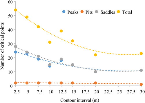
Figure 7. Relationship between the number of feature points and the contour interval in hilly area.

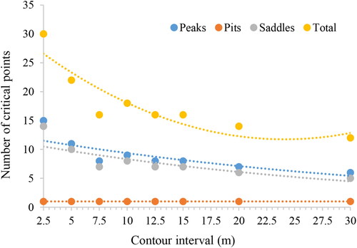
Table 3. Statistical results for mountainous area.

Contour interval (m)	Peaks	Pits	Saddles	Total	Euler’s equation
2.5	24	2	28	54	−2
5	23	2	24	49	1
7.5	19	2	21	42	0
10	14	2	15	31	1
12.5	18	2	19	39	1
15	15	2	15	32	2
20	10	2	10	22	2
30	11	1	11	23	1

Table 4. Statistical results for hilly area.

Contour interval (m)	Peaks	Pits	Saddles	Total	Euler’s equation
2.5	15	1	14	30	2
5	11	1	10	22	2
7.5	8	1	7	16	2
10	9	1	8	18	2
12.5	8	1	7	16	2
15	8	1	7	16	2
20	7	1	6	14	2
30	6	1	5	12	2

Due to the central role of peaks, saddles and pits in the fields of surface network construction and cartographic synthesis, Takahashi et al. (1995) argued that the non-degenerate feature points extracted from DEMs should conform to Euler’s equation, as mentioned in Section 1. Therefore, they suggested introducing a global virtual pit and decomposing the degraded pits to satisfy Euler’s equation. However, as shown in Tables 3 and 4, the numbers of feature points extracted from the DEMs usually fail to satisfy Euler’s equation, especially at small contour intervals.

In practice, considering the data characteristics of DEMs and their practical application requirements, there is no need for the numbers of feature points to satisfy Euler’s equation. This can be explained as follows. (1) The prerequisite of Euler’s equation is a smooth surface or a dense discrete surface with high precision, whereas a DEM with a discrete regular grid or irregular grid surface does not satisfy this condition (Takahashi et al. 1995; Jeong et al. 2014). The algorithm proposed in this paper is based on the shapes and relationships between contour lines, so it is not subject to this constraint. (2) The introduction of a virtual pit or the decomposition of degraded saddles will lead to the appearance of topographic features without any morphological significance (Čomić et al. 2014). In contrast, various feature points can be naturally identified through the spatial topological relationship between contour lines, which is more consistent with human visual cognition and judgment. (3) In the construction of the surface network, it is usually assumed that a saddle point is associated with two steepest descent gradients (valley lines) and two steepest ascent gradients (ridge lines), which imposes more stringent requirements on the number of feature points.

3.3.2. Contour interval and location of terrain feature points

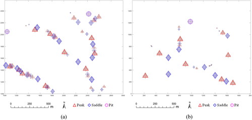
From a local viewpoint, Figure 8(a,b) show the spatial locations of the feature points extracted by the proposed algorithm with contour intervals of 20, 10 and 5 m in the same areas of the mountainous and hilly DEMs, respectively. As can be seen, in both DEMs, the number of extracted feature points gradually increases with the decrease in the contour interval, indicating that more details of the terrain are revealed. However, the spatial positions of the extracted feature points in the focal region remain unchanged, without any offset. For example, take point P in Figure 8(a), which is an extracted feature point deemed to be a peak. In the areas marked by blue ellipses, when the contour interval is reduced to 5 m, more feature points around point P are extracted, but the spatial position of the feature point P remains unchanged.

Figure 8. Spatial positions of feature points extracted with different contour intervals in a local area. (a) Mountainous area; (b) hilly area.

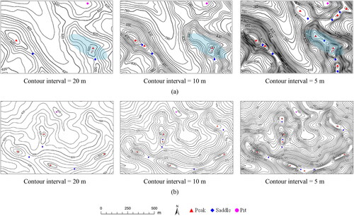
According to the morphological mathematical model of feature points, a contour line containing a feature point will shrink to a point as the contour interval is reduced. In the region surrounded by a contour line, the peak can be regarded as the local highest point and the pit as the local lowest point, while there is only one self-intersecting contour line across the saddle. This implies that the position of a feature point remains constant irrespective of the contour interval. That is, although the numbers of extracted feature points depend on the contour interval, the locations of these feature points remain unchanged. Figure 9 presents the superimposed results of peak, pit and saddle extraction at different contour intervals in the two sample areas. In both the mountainous area and the hilly area, the positions of feature points coincide perfectly, despite the differences in their quantitative properties.

Figure 9. Spatial distribution of feature points extracted at different contour intervals. The black crosses indicate the locations of feature points, and the sizes of the symbols correspond to the contour intervals at which the feature points are extracted (2.5 m, 5 m, 7.5 m, 10 m, 12.5, 15, 20 and 30 m), i.e. the smaller the symbol, the smaller the contour interval. (a) Mountainous area; (b) hilly area.

4. Discussion

In this section, based on a DEM with 10-meter resolution and 5-meter contour interval, the effectiveness and correctness of our proposed algorithm are further discussed. Using manually extracted results as references, our results have been compared with those obtained from existing methods. These comparative analyses aim to present the strengths and improvements our algorithm offers in the terrain feature extraction.

4.1. Selection of existing algorithms

Many geomorphometric analysis methods and techniques have been proposed to extract terrain features from DEM, including eight-neighbour method (Peucker and Douglas 1975), Geomorphon (Jasiewicz and Stepinski 2013), Topographic Position Index (Weiss 2001), Multiscale Quadratic Polynomial Estimation (Wood 1996), GIS hydrological analysis method (ESRI, 2020) and etc. The first four belong to a local window analysis and the last can be regarded as a vector analysis model. Considering the methods of Geomorphon, Topographic Position Index and Multiscale Quadratic Polynomial Estimation need experiments to determine the best scaling parameters, this study selects the classical eight-neighbour method and hydrological analysis method as the comparisons.

Based on a fixed 3 × 3 moving window, the Peucker algorithm extracts feature points from the change in height difference between the central grid cell and its surrounding eight grid cells (Peucker and Douglas 1975). GIS hydrologic analysis is a procedural method including a series of operational steps (ESRI, 2020). For peaks and pits, statistical analysis with a variable neighborhood window is used. For saddles, it is considered that a saddle point is a topographic feature point with the local highest point in one direction and the local lowest point in the other direction. Therefore, a ridge line is extracted by tracing the local highest points and a valley line is extracted by tracing the local lowest points. Finally, the saddle is extracted at the intersection of the ridge line and valley line (Zhang et al. 2011; Li et al. 2022; Hu et al. 2022).

Figures 10(a–d) and 11(a–d) show the extracted results of the manual method, the method proposed in this study, Peucker algorithm and GIS hydrological analysis method in the two study areas respectively. Using the accuracy metrics of completeness, correctness and quality, statistical analyses of the feature points extracted by different methods are presented in Tables 5 and 6.

Figure 10. Comparative results of feature point extraction with different methods in a mountainous area (the contour interval is 5 m). (a) Manual extraction method; (b) method proposed in this study; (c) Peucker algorithm; (d) GIS hydrological analysis method.

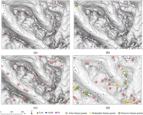
Figure 11. Comparative results of feature point extraction with different methods in a hilly area (the contour interval is 5 m). (a) Manual extraction method; (b) method proposed in this study; (c) Peucker algorithm; (d) GIS hydrological analysis method.

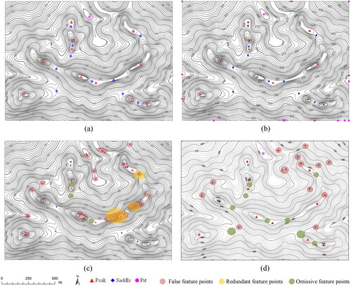
Table 5. Accuracy comparison results of different methods in mountainous area.

Methods	Peaks	Saddles	Pits
Manual method	23	25	2
Proposed method	23/0/0/0	24/0/0/1	2/0/0/0
	(100%, 100%, 100%)	(100%, 96%, 100%)	(100%, 100%, 100%)
Peucker algorithm	38/0/15/0	60/39/4/8	4/2/0/0
	(60.5%, 100%, 60.5%)	(17.3%, 52.9%, 15%)	(50%, 100%, 50%)
GIS hydrological analysis method	20/1/0/4	43/17/6/5	2/0/0/0
	(95%, 82.6%, 79.2%)	(46.5%, 80%, 41.7%)	(100%, 100%, 100%)

Contour interval is set 5 m. Digit in A/B/C/D represent the number of totals, false, redundant, and omissive feature points respectively. Digit in (A, B, C) denotes the accuracy metric of completeness, correctness and quality respectively.

Table 6. Accuracy comparison results of different methods in hilly area.

Methods	Peaks	Saddles	Pits
Manual method	11	10	1
Proposed method	11/0/0/0	10/0/0/0	1/0/0/0
	(100%, 100%, 100%)	(100%, 100%, 100%)	(100%, 100%, 100%)
Peucker algorithm	29/18/0/0	44/37/0/3	1/0/0/0
	(37.9%, 100%, 37.9%)	(15.9%, 70.0%, 14.0%)	(100%, 100%, 100%)
GIS hydrological analysis method	14/3/0/0	12/11/0/9	1/0/0/0
	(78.5%, 100%, 78.5%)	(21.4%, 25%, 13.0%)	(100%, 100%, 100%)

Contour interval is set 5 m. Digit in A/B/C/D represent the number of totals, false, redundant, and omissive feature points respectively. Digit in (A, B, C) denotes the accuracy metric of completeness, correctness and quality respectively.

4.2. Accuracy of the extracted peaks and pits

As a peak can be seen as the highest point in a local region and a pit can be seen as the lowest point in a local region, then irrespective of whether a fixed 3 × 3 moving window or a k × k (k is odd) variable neighborhood window is used, the principle is to determine whether the central grid cell is the elevation extremum of its neighborhood (Wood 1996). Therefore, the Peucker algorithm and GIS hydrologic analysis method can identify peaks and pits comparatively correctly, but these may be accompanied by some redundant, false, and omissive points for DEM error and size of local window (Li et al. 2022). As shown in Figures 10 and 11, our results are consistent with those of the manual method in both study areas, except for the redundant feature points caused by the boundary effect (as discussed in Section 3.2).

Statistical analyses in Tables 5 and 6 show a consistent conclusion with the above visual analysis. Compared with the manual method results, although the pit numbers are similar, the peak numbers extracted by the three methods are significantly different both in the two study areas. In particular, Peucker algorithm and GIS hydrological analysis method show almost 100% correctness but the completeness is relatively low (Peucker algorithm with 60.5% and 37.9%, GIS hydrological analysis method with 95% and 78.5% in Table 5 and Table 6, respectively) due to the generation of a great number of redundant, false, and omissive peaks. This is because they are both based on a moving window method. When a neighborhood window moves continuously cell by cell throughout the DEM, which results in overlapping of neighborhood windows between adjacent DEM cells, the contextual information of adjacent windows is not considered while evaluating the current window attributes (Xiong et al. 2021; Hu et al. 2022).

While in contour topographic maps, a peak, as well as a pit, is characterized by a closed contour line. Although feature contour lines of local peaks and pits may form multiple closed contours, there is only one closed contour containing a peak or pit (Imhof 1982). Being based on contour lines generated from a DEM, the proposed approach is not confined to an analytical visual field within a neighborhood window, nor does it need to determine the window size under different terrain conditions through experiments. Due to the global attribute of contour lines and their explicit topological relationships (Guilbert 2013, 2021), the results of the proposed method are satisfactory with the correctness and completeness up to almost 100%, as shown in Tables 5 and 6.

4.3. Accuracy of the extracted saddles

In terms of spatial distribution, saddles and peaks appear alternately along ridge lines, while saddles and pits appear alternately along valley lines (Takahashi et al. 1995), but for contour lines, the point shared by two or more contours can be defined as a saddle (Guilbert 2021). Compared with a simply closed contour morphology of peaks and pits, the surface shape of saddles is more complex, resulting in a large difference in the numbers of saddles among three algorithms. As shown in Tables 5 and 6, the saddles extracted by the three algorithms are 24, 60 and 44 respectively in mountainous areas, while 10, 44 and 12 respectively in hilly areas. While Peucker algorithm and GIS hydrological analysis not only have lower correctness, but also lower completeness.

In the Peucker algorithm, a saddle point is defined as follows. In a local window, first, the elevation differences between the center point and its neighbors are calculated, and then the changes in the sign of the differences are counted. If the number of changes is four and the sum of the positive and negative differences is greater than the threshold, the center point can be seen as a saddle. As shown in Figures 10(c) and 11(c), for hilltop regions, slope surfaces and other relatively gentle areas, it is easy to meet such a condition. Also, noises in DEMs may lead to a large number of false saddles, 39 and 37 in the two study areas respectively (as shown in Tables 5 and 6). Although this can be controlled by setting the threshold, determining the threshold value is not easy (Florinsky 2009; Zhao et al. 2014). Moreover, a saddle is located between two connected peaks, where the terrain is gentle and relatively open. Thus, a saddle point may be omitted due to the visual field limitation of a local window (Xiong et al. 2021). Tables 5 and 6 shows that 8 are omissive in mountainous area and 3 in hilly area. Furthermore, the overlapping of neighborhood windows between adjacent DEM cells may result in redundant saddles (e.g. 4 redundancies in mountainous area). As a result, the correctness and completeness of Peucker algorithm are very low in both two study areas (52.9% and 17.3% in mountainous area, 15.9% and 70.0% in hilly area).

As seen in Figures 10(d) and 11(d), similar to the Peucker algorithm, the GIS hydrological simulation method is with 80% correctness and 46.5% completeness in mountainous area, and with 25% correctness and 21.4% completeness in hilly areas (as shown in Tables 5 and 6). This method produces a number of false, omitted and redundant saddles. In GIS hydrological analysis, the delineation of ridge lines (valley lines) is achieved through the simulation of runoff concentration, and this process entails a filtering technique that mitigates the impact of negative terrain (positive terrain). This technique, while effective in extracting ridge lines (valley lines), often leads to discontinuities along these features. Consequently, the resulting fragmented lines may not consistently converge at saddle area. This inconsistency can give rise to inaccuracies, manifesting false saddles or omitted saddles in certain regions (Huang et al. 2020; Hu et al. 2022).

Unlike the Peucker algorithm and GIS hydrological analysis method, the proposed algorithm extracts saddles through the topological relationship between contour lines. Seeing Tables 5 and 6, our extracted saddle points are almost consistent with the manual methods, and the accuracies of the two study areas are almost 100%. The only omissive saddle is in the upper left corner of Figure 10(b). When the contour interval is small, the method is prone to producing closed contour lines at the boundary because of the compact contour group, resulting in omitted saddles near the boundary. Even so, the global properties of contour lines can overcome the limitation of analytical visual fields within a neighborhood window, and the extracted saddles are more in accord with the cognitive rules of geomorphology. Our extraction method ensures the spatial correspondence between saddles, peaks and pits, and effectively avoids the appearance of false, omitted and redundant saddles. Another advantage is that contour lines are not sensitive to the data noise of DEMs (Li et al. 2022), which can reduce the influence of DEM errors on feature point extraction.

4.4. Limitations of the proposed method

Despite the important contributions of this study, it has also certain limitations. In contrast to the traditional approaches, our approach has the contour interval as the only variable, with no need to set various threshold values. This is an important advantage of the method, but also creates the problem of how to choose an appropriate contour interval (as shown in Figure 5). Considering that the DEMs with different resolutions in most early products generally corresponded to topographic maps of different scales, a feasible approach is to learn from the settings of the basic contour intervals of topographic maps. For example, for DEMs with a 25 m resolution published in China, the contour interval of the corresponding topographic maps is between 10 and 20 m with different terrain types. Thus, if the Shuttle Radar Topography Mission (SRTM) DEM or the Advanced Spaceborne Thermal Emission and Reflection Radiometer (ASTER) Global DEM with a 30 m resolution were used in this approach, the contour interval could be set as 10–20 m according to the similar correspondence rules between the resolution of DEMs and the topographic maps with known contour intervals. In the future, we will carry out a deeper study of the selection of the contour interval. Further investigation is required to examine this proposed method in more detail.

5. Conclusion

In this study, a new method of automatically extracting topographic feature points from DEMs is developed based on geomorphic intuition regarding terrain feature points and the topological relationships of contour lines. Combined with constraints on terrain morphological features, morphological mathematical models of peaks, saddles and pits were constructed with feature contour lines as the core, and the corresponding interpretation algorithms were designed. Compared with existing methods, the proposed approach has a higher accuracy and effectively avoids the occurrence of false, omitted and redundant feature points.

The principal conclusions of this study are summarized as follows:

1. Considering the inherent discreteness and presence of data noise in DEMs, the topographic morphology emerges as a critical factor in the successful identification of topographic terrain feature points from DEMs.

2. Through the contour topological relationships, which naturally contain topographic features, our methodology enables the precise and comprehensive extraction of feature points from DEMs. This approach markedly outperforms existing techniques by efficiently avoiding the generation of erroneous feature points often associated with the local window method, thereby eliminating omission and redundancy. The outcomes achieved through our method demonstrate a high level of correctness and completeness.

3. The contour interval is the only variable of this algorithm once the resolution of the DEM is determined. It is observed that an increase in the contour interval results in a reduction of the number of topographic feature points, though this does not impact their spatial positioning.

4. Our proposed method adopts a global strategy, effectively overcoming the limitations posed by the narrow perspective of local window approaches. It negates the need for setting various threshold values, offering a more streamlined and efficient process for the extraction of topographic features.

Acknowledgments

Special thanks go to Maan Habib, who provided the test datasets, and the reviewers, who made valuable comments on the study.

Data availability statement

The data supporting the findings of this study are available upon reasonable request from the authors.

Disclosure statement

The authors report there are no competing interests to declare.

Additional information

Funding

This work was supported by the National Natural Science Foundation of China (NSFC) (No. 41971364 and No. 41371421).

References

- Ai T, Li J. 2010. A DEM generalization by minor valley branch detection and grid filling. ISPRS J Photogramm Remote Sens. 65(2):198–207. doi: 10.1016/j.isprsjprs.2009.11.001.
- Anders NS, Seijmonsbergen AC, Bouten W. 2013. Geomorphological change detection using object-based feature extraction from multi-temporal LIDAR data. IEEE Geosci Remote Sensing Lett. 10(6):1587–1591. doi: 10.1109/LGRS.2013.2262317.
- Arundel S, Li W, Zhou X. 2018. The effect of resolution on terrain feature extraction. PeerJ Preprints. 6:e27072. doi: 10.7287/peerj.preprints.27072v1.
- Bolongaro-Crevenna A, Torres-Rodriguez V, Sorani V, Frame D, Ortiz MA. 2005. Geomorphometric analysis for characterizing landforms in Morelos State Mexico. Geomorphology. 67:407–422. doi: 10.1016/j.geomorph.2004.11.007.
- Cheng L, Guo Q, Fei L, Wei Z, He G, Liu Y. 2022. Multi-criterion methods to extract topographic feature lines from contours on different topographic gradients. Int J Geo Info Sci. 36(8):1629–1651. doi: 10.1080/13658816.2021.2024194.
- Clarke KC, Romero BE. 2017. On the topology of topography: a review. Cartograp Geograp Info Sci. 44(3):271–282. doi: 10.1080/15230406.2016.1164625.
- Cromley RG. 1991. Hierarchical methods of line simplification. Cartography and Geographic Information Systems. 18(2):125–131. doi: 10.1559/152304091783805563.
- Dikau R. 2020. The application of a digital relief model to landform analysis in geomorphology. In: Raper J, editor. Three dimensional applications in GIS. London: Taylor & Francis; p. 51–77. doi: 10.1201/9781003069454-5.
- ESRI. 2020. ArcGIS Pro: Release 2.4. Redlands, CA: Environmental Systems Research Institute.
- Etzelmüller B. 2000. On the quantification of surface changes using grid-based digital elevation models (DEMs). Trans GIS. 4(2):129–143. doi: 10.1111/1467-9671.00043.
- Florinsky IV. 2009. Computation of the third‐order partial derivatives from a digital elevation model. Int J Geograph Info Sci. 23(2):213–231. doi: 10.1080/13658810802527499.
- Florinsky IV. 2016. Digital terrain analysis in soil science and geology. (2nd ed.). Amsterdam: Academic Press.
- Guilbert E. 2013. Multi-level representation of terrain features on a contour map. Geoinformatica. 17(2):301–324. doi: 10.1007/s10707-012-0153-z.
- Guilbert E. 2021. Surface network extraction from high resolution digital terrain models. JOSIS. 22(22):33–59. doi: 10.5311/JOSIS.2021.22.681.
- Habib M. 2021. Evaluation of DEM interpolation techniques for characterizing terrain roughness. Catena. 198:105072. doi: 10.1016/j.catena.2020.105072.
- Heckmann T, Schwanghart W, Phillips JD. 2015. Graph theory-recent developments of its application in geomorphology. Geomorphology. 243:130–146. doi: 10.1016/j.geomorph.2014.12.024.
- Hu J, Luo M, Bai L, Duan J, Yu B. 2022. An integrated algorithm for extracting terrain feature-point clusters based on DEM data. Remote Sensing. 14(12):2776. doi: 10.3390/rs14122776.
- Huang N, Yang X, Liu HL. 2020. A method of saddle point extraction based on contour spatial relationship. J Geo-Info Sci. 22(3):410–421. doi: 10.12082/dqxxkx.2020.190572.
- Imhof E. 1982. Cartographic relief representation. Berlin: De Gruyter. doi: 10.1515/9783110844016.
- Jasiewicz J, Stepinski TF. 2013. Geomorphons – a pattern recognition approach to classification and mapping of landforms. Geomorphology. 182:147–156. doi: 10.1016/j.geomorph.2012.11.005.
- Jeong MH, Duckham M, Kealy A, Miller HJ, Peisker A. 2014. Decentralized and coordinate-free computation of critical points and surface networks in a discretized scalar field. Int J Geograph Info Sci. 28(1):1–21. doi: 10.1080/13658816.2013.801578.
- Li M, Wu T, Li W, Wang C, Dai W, Su X, Zhao Y. 2022. Terrain skeleton construction and analysis in Loess Plateau of Northern Shaanxi. IJGI. 11(2):136. doi: 10.3390/ijgi11020136.
- MacMillan RA, Shary PA. 2009. Landforms and landform elements in geomorphometry. Develop Soil Sci. 33:227–254. doi: 10.1016/S0166-2481(08)00009-3.
- Mokarram M, Shaygan M, Sathyamoorthy D. 2018. Using DEM and GIS for evaluation of groundwater resources in relation to landforms in the Maharlou-Bakhtegan watershed, Fars province, Iran. J Water Land Develop. 37(1):121–126. doi: 10.2478/jwld-2018-0031.
- Neyestani M, Sarmadian F, Jafari A, Keshavarzi A, Sharififar A. 2021. Digital mapping of soil classes using spatial extrapolation with imbalanced data. Geoderma Regional. 26:e00422. doi: 10.1016/j.geodrs.2021.e00422.
- Peucker TK, Douglas DH. 1975. Detection of surface-specific points by local parallel processing of discrete terrain elevation data. Comput Graph Image Process. 4(4):375–387. doi: 10.1016/0146-664X(75)90005-2.
- Pike RJ. 2000. Geomorphometry diversity in quantitative surface analysis. Prog Phys Geograph. 24(1):1–20. doi: 10.1177/030913330002400101.
- Rutzinger M, Höfle B, Kringer K. 2012. Accuracy of automatically extracted geomorphological breaklines from airborne LIDAR curvature images. Geografiska Annaler: Series A, Phys Geograph. 94(1):33–42. doi: 10.1111/j.1468-0459.2012.00453.x.
- Samsonov T. 2022. Granularity of digital elevation model and optimal level of detail in small-scale cartographic relief presentation. Remote Sensing. 14(5):1270. doi: 10.3390/rs14051270.
- Schmidt J, Allan H. 2004. Fuzzy land element classification from DTMs based on geometry and terrain position. Geoderma. 121(3–4):243–256. doi: 10.1016/j.geoderma.2003.10.008.
- Schneider B. 2005. Extraction of hierarchical surface networks from bilinear surface patches. Geog Anal. 37(2):244–263. doi: 10.1111/j.1538-4632.2005.00638.x.
- Schneider B, Wood J. 2004. Construction of metric surface networks from raster‐based DEMs. In: Rana S, editor. Topological data structures for surfaces: an introduction for geographical information science. London, UK: John Wiley & Sons; p. 53–70. doi: 10.1002/0470020288.ch4.
- Song D, Yue T, Du Z. 2011. Constructing contour tree and DEM construction of high fidelity. J Image Graph. 16(7):1255–1261. doi: 10.11834/jig.20110710.
- Takahashi S, Ikeda T, Shinagawa Y, Kunii TL, Ueda M. 1995. Algorithms for extracting correct critical points and constructing topological graphs from discrete geographical elevation data. Proc Comput Graphics Forum. 14(3):181–192. doi: 10.1111/j.1467-8659.1995.cgf143_0181.x.
- Tavares DCR, Mazzoli R, Bagli S. 2019. Limitations posed by free DEMs in watershed studies: the case of river Tanaro in Italy. Frontiers in Earth Science. 7:141. doi: 10.3389/feart.2019.00141.
- Wang J, Yu Z. 2009. A Morse-theory based method for segmentation of triangulated freeform surfaces. Advances in Visual Computing: 5th International Symposium. Las Vegas, Nevada. Proceedings, Part II 5. p. 939–948. doi: 10.1007/978-3-642-10520-3_90.
- Weiss A. 2001. Topographic position and landforms analysis. Poster presentation Esri User Conference, San Diego, CA. Vol. 200.
- Wilson JP. 2018. Environmental applications of digital terrain modeling. Chichester, UK: John Wiley & Sons. doi: 10.1002/9781118938188.
- Wood J. 1996. The geomorphological characterisation of digital elevation models. United Kingdom: University of Leicester.
- Wood J, Rana S. 2000. Constructing weighted surface networks for the representation and analysis of surface topology. Proceedings 5th International Conference on GeoComputation. Chatham, UK. p. 23–25.
- Xiong L, Tang G, Yang X, Li F. 2021. Geomorphology-oriented digital terrain analysis. Progress and perspectives. J Geogr Sci. 31(3):456–476. doi: 10.1007/s11442-021-1853-9.
- Zhang W, Tang G, Tao Y. 2011. An improved method to saddles extraction based on runoff concentration simulation in DEM. Sci Survey Map. 36(1):158–159. 163. doi: 10.16251/j.cnki.1009-2307.2011.01.026.
- Zhang S, Zhao B, Erdun E. 2014. Watershed characteristics extraction and subsequent terrain analysis based on digital elevation model in flat region. J Hydrol Eng. 19(11):04014023. doi: 10.1061/(ASCE)HE.1943-5584.0000961.
- Zhao P, Zhang LC, Zhang WS, Wan MY. 2014. A topographic feature line extraction algorithm based on terrain curvature. J Geomat Sci Tech. 31(1):13–17. doi: 10.3969/j.issn.1673-6338.2014.01.004.
- Zhou X, Li W, Arundel ST. 2019. A spatio-contextual probabilistic model for extracting linear features in hilly terrains from high-resolution DEM data. Int J Geograph Info Sci. 33(4):666–686. doi: 10.1080/13658816.2018.1554814.
- Zhou W, Peng R, Dong J, Wang T. 2018. Automated extraction of 3D vector topographic feature line from terrain point cloud. Geocarto Int. 33(10):1036–1047. doi: 10.1080/10106049.2017.1325521.