Hyperspectral identification of travertine state in Huanglong by the PSO-BPNN method

Abstract

The Huanglong Scenic and Historic Interest Area in China, a UNESCO World Heritage Site, is famous for its large-scale, diverse, intricately structured, and brightly colored surface travertine landscapes. However, severe degradation of the Huanglong travertine formations, such as blackening and algae erosion, has occurred in recent years, necessitating monitoring and identification. We collected hyperspectral reflectance data of the travertine formations in different states and bare ground using a ground-based hyperspectral radiometer (PSR-2500) from ASD company. After conducting a correlation analysis between the hyperspectral reflectance data and the travertine formations, we identified healthy travertine formations, blackened travertine formations, travertine formations affected by algae erosion, and bare ground. The Siamese network method was employed to generate data labels, and the spectral features of the travertine formations were extracted by combining the sensitive bands with pre-processed and reduced data. The PSO-BPNN classifier was developed by optimizing the back propagation neural network (BPNN) using the particle swarm optimization algorithm (PSO). To verify the effectiveness of PSO-BPNN in accurately distinguishing different states of travertine formations, we compared its performance with that of BPNN using three performance indices. Finally, the proposed method was applied to the real-world hyperspectral image data collected by the Micro-Hyperspectral imaging instrument to classify the travertine formations in different states and bare ground. The test set demonstrated good overall performance, with an average overall accuracy (OA) of 0.93, F1-score of 0.92, and Kappa coefficient of 0.97.

Keywords:

• Travertine
• hyperspectral
• spectral feature extraction
• particle swarm algorithm
• back propagation neural network

1. Introduction

Travertine is an essential record of fluid flow in the earth’s crust in the past, which records fluid migration through tectonic activity and climate change, and large-scale travertine landscapes are also of high tourism value as a natural heritage. However, in recent years, due to global climate change and anthropogenic factors, travertine is vulnerable to damage and even degradation (Li et al. 2018; Ricketts et al. 2019; Jiang et al. 2021; Liu et al. 2021), which not only destroys the landscape of travertine but also deteriorates the local geologic conditions, which can easily lead to rock collapse and other geologic disasters. In the study area, the most typical travertine landscape is Huanglong in China, where the travertine is deposited because of the oversaturation and overflow of calcium carbonate under the action of the deep pressure of the earth (Liu et al. 2023). There are many kinds of travertine in Huanglong, which can be classified into porous travertine, dense travertine, and clastic travertine from the cause of travertine, and can be classified into striated travertine, plate travertine, and sponge travertine in the depositional morphology (Qiao et al. 2022). This paper divides the travertine in Huanglong into healthy travertine, blackened travertine, and algal erosion travertine based on the state of the travertine. Blackened travertine and algal erosion travertine are the typical features of the degradation of the travertine. Blackened travertine is mainly formed due to the oxidation of iron, fierce elements, or organic matter contained in the absence of water (Qiao et al. 2022). Algae-eroded travertine is mainly formed due to the eutrophication of the water body, which leads to the growth of algae attached to the travertine. Excessive growth of algae attached to the travertine will destroy the microenvironment of the travertine deposition, which affects the denseness of the travertine depositional structure (Rao et al. 2023).

Hyperspectral travertine identification refers to utilizing variations in hyperspectral curves of different travertine states to identify and discern travertine deposits. After preprocessing and feature extraction of hyperspectral data, classification and identification can be performed based on the extracted features (Lin et al. 2020; Liu et al. 2022), For example, A. J. Brown uses automatic discovery and curve fitting of absorption bands in hyperspectral data can enable the analyst to identify materials present in a scene by comparison with library spectra(Brown. 2006). Hyperspectral identification methods significantly improve efficiency and save labor compared to traditional field surveys (Sun et al. 2021), For example, A. J. Brown have analyzed spectra from CRISM images and used co-located HiRISE images in order to further characterize these carbonate-bearing units (Brown et al. 2010). Furthermore, hyperspectral data can detect materials with diagnostic spectral absorption features, which help study the composition of substances (Yang et al. 2022). Many existing studies have analyzed or identified rock minerals using hyperspectral data. For example, a combination of hyperspectral images and deep learning methods has successfully classified 13 rock lithologies (Galdames et al. 2022). Researchers have established estimation models using rock spectral data and modified normalized difference index in estimating iron content in rocks (Wang et al. 2021). In some cases, spectral data is transformed into first and second-order derivatives and combined with partial least squares support vector machines to establish estimation models for evaluating material content in rocks (Cui et al. 2019).

Upon addressing the challenges of processing high-dimensional hyperspectral feature data, it is necessary to classify and identify the extracted information (Yadav et al. 2019; Jiang et al. 2021). Currently, classification methods can be divided into two categories. One approach involves conducting extensive experiments and verifications based on extracted hyperspectral feature information, summarizing discriminant criteria, and using discriminant criteria for data classification and identification. Existing studies have developed discriminant methods based on three spatial autocorrelation indices to identify water bodies in Landsat images or using comparative discriminant formulas based on infrared spectra to analyze and identify exposed coal (Xu et al. 2020). While these discriminant methods achieve good classification results on existing data sets, their accuracy cannot be guaranteed for unknown data. Another approach involves utilizing machine learning or deep learning methods to learn from feature data sets to obtain models for classification and identification (Gao et al. 2021; Liu et al. 2021). Machine learning or deep learning methods commonly include backpropagation neural networks, support vector machines (SVMs), and convolutional neural networks (CNNs) (Zhao et al. 2019; Yu et al. 2021; Qiao et al. 2022). These methods are well-established. For instance, SVM has been successfully applied in classifying hyperspectral images of 100 kinds of flowers.

In this study, we will utilize data collected by the PSR-2500 hyperspectral spectrometer to conduct data preprocessing, feature extraction, and recognition model establishment for travertine deposits. After evaluating the established recognition model, we will apply it to data collected by the Micro-Hyperspectral imaging system and assess the results to validate the model’s performance further.

2. Materials and methods

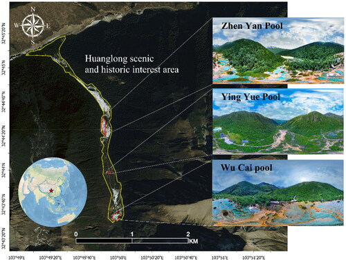
The research area of this study is situated within the Huanglong Scenic Area in SONGPAN County, Aba Tibetan and Qiang Autonomous Prefecture, Sichuan Province, China. It is renowned for its surface travertine deposits, which are the defining feature of the Huanglong landscape. The main attractions are concentrated in the Huanglong Valley, spanning approximately 3.6 kilometers. The scenic area is adorned with extensive carbonate travertine deposits resembling terraced formations and a majestic golden dragon. Designated as a UNESCO World Natural Heritage site, the area has unfortunately experienced significant degradation in its travertine resources, including phenomena such as travertine darkening and erosion caused by algae (Sun et al. 2021). The location of the research area is illustrated in Figure 1.

Figure 1. Research area.

2.1. Data collection

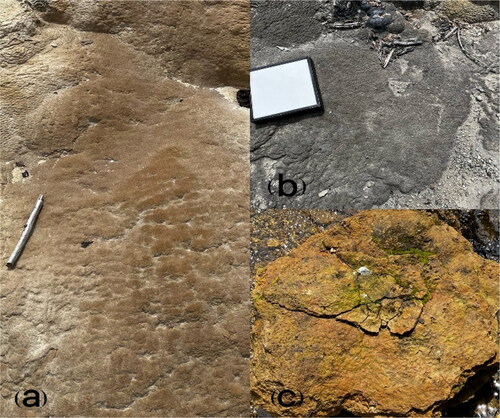
The PSR-2500 field spectrometer and Micro-Hyperspectral imaging spectrometer were used to collect hyperspectral data of three types of travertine deposits and bare soil at various locations in the Huanglong Scenic Area, including the Colorful Pool, Reflecting Moon Pool, and Competitive Color Pool. The three types of travertine deposits are shown in Figure 2. Healthy travertine deposits are mainly yellow or yellowish-gray in color, often appearing as block-like sedimentary rocks with visible travertine particles. Blackened travertine exhibits a black or dark gray layout, and it is harder than healthy travertine, with frequent biological traces on its surface. Travertine erosion caused by algae is often accompanied by green algae on the surface, mainly found in areas with high water flow, and the surface appears smooth with cracks.

Figure 2. (a) Healthy travertine; (b) blackened travertine; (c) algal erosion of travertine.

2.1.1. Data acquisition of PSR-2500 ground spectrometer

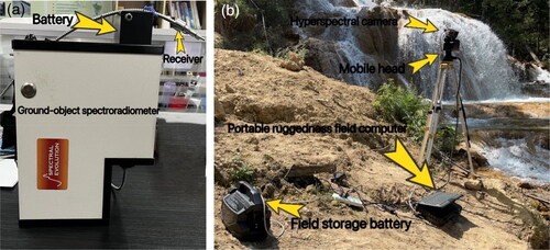
The PSR-2500 field spectrometer primarily comprises a light source, light path, spectrometer, and control system. During field data collection, sunlight was used as the light source, while daylight lamps were used in laboratory settings. The light path is an essential part of the field spectrometer, guiding the light beam emitted by the light source into the spectrometer. The spectrometer, which is the field spectrometer’s core component, measures the target surface’s spectral reflection. The control system can be operated through the built-in buttons on the spectrometer or controlled via the DWIN software when connected to a computer. The appearance of the PSR-2500 field spectrometer is depicted in Figure 3(a), and the collected data is based on specific points of the target surface.

Figure 3. (a) PSR-2500 spectrometer; (b) micro-hyperspace imaging spectrometer.

During the field data collection of travertine high spectral reflectance using the PSR-2500 field spectrometer, it is necessary to perform whiteboard reflectance light correction. A whiteboard was placed at the position where the samples were collected, and the angle of the sunlight reflecting from the whiteboard was selected. By using the collection device, the spectrometer obtained the complete reflection light from the whiteboard. Subsequently, high spectral reflectance data of the samples were collected at the same position as the whiteboard. Each sample point was collected ten times, and the instrument parameters are shown in Table 1. The collected spectral curves are shown in Figure 4. When analyzing the high spectral reflectance curves of the three travertine and bare soil types, noticeable differences were observed in the average reflectance curves of the four categories. The reflectance curve of darkened travertine is entirely different from the other three curves, with an increase in reflectance before the 500 nm band, followed by a continuous decrease until the approximately 1800 nm band, and a general upward trend. Travertine erosion caused by algae, which often appears near water flows, has higher reflectance values than the other three types. The reflectance curves of healthy travertine and bare soil are very similar. Still, healthy travertine’s overall reflectance is higher than bare soil. Hyperspectral curve characteristics of travertine in different states above provide a basis for using high spectral reflectance data to identify different conditions of travertine.

Figure 4. Hyperspectral reflectance.

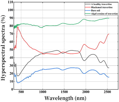
Table 1. Main technical parameters of the PSR-2500 spectrometer.

Nominal measuring range	Actual measuring range	Wavelength accuracy	Spectral resolution
350–2500 nm	334.3–2535.9 nm	5 nm	< =3.5 nm(350–1000 nm)；< =22 nm(1000 − 2500 nm)

2.1.2. Micro-hyperspace hyperspectral imager data acquisition

We used the Micro-Hyperspace imaging spectrometer to collect hyperspectral image data at locations with good exposure of travertine deposits in the Huanglong Scenic Area. The observations were conducted under clear, windless, and partially cloudy weather conditions. Observational stations were set up for data collection. The hyperspectral imaging system consisted of the hyperspectral imaging spectrometer, a portable rugged notebook computer, an outdoor mobile platform, and a calibration whiteboard, as shown in Figure 3(b). The hyperspectral camera consisted of the imaging acquisition unit (Micro-Hyperspace VNIR), a CCD camera, and a lens, with sunlight as the light source. The specific parameters and performance indicators of the imaging spectrometer can be found in Table 2. The data collection was performed using the accompanying software Spectral View. During the observations, the scanning platform moved at 0.258 cm/s, matching the resolution speed. Before image capture, the camera was focused and the white calibration was conducted for the whiteboard spectra to correct for bright current and the blackboard calibration for dark current. The data collected were acquired based on the surface of the objects. Compared to the PSR-2500 field spectrometer, the Micro-Hyperspace imaging spectrometer not only captured spectral information but also obtained image information. The collected images are shown in Figure 5.

Figure 5. Hyperspectral image data collected by the Micro-hyperspace hyperspectral imaging spectrometer and spectral reflectance curve of a specific point.

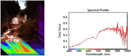
Table 2. Micro-hyperspace hyperspectral imaging instrument parameters.

Parameter	Value
Model	Micro-hyperspace VNIR series
Splitting element	Aberration-corrected concave reflection holographic grating
Wavelength range	400–1000 nm
Pixel size	7.4 μm
Spectral resolution	5 nm
Slit width	10.5 nm
Spectral channels	325
Spatial channels	1004
Data format	Data/Hyperspectral image data
Photosensitive Element	Silicon CCD
Weight	0.7 kg
Manufacturer	Headwall photonics Inc.

2.2. Method

2.2.1. Preprocessing method

We employed the Savitzky-Golay algorithm with a sliding filtering window size of 7 to remove noise from the spectral data (Romo-Cárdenas et al. 2018). Additionally, we utilized the Multiplicative Scatter Correction (MSC) algorithm to eliminate spectral differences caused by variations in scattering levels. The MSC principle involves correcting baseline shifts and offsets in the original spectral data by using the mean of the raw spectral data as the ‘ideal data’ (Cen et al. 2022; Diago-Cisneros 2022).

During the data collection process of the PSR-2500 hyperspectral instrument, issues may arise where the data becomes difficult to identify due to capture errors and disorganized storage. This study used a Siamese neural network algorithm to address this problem. The process is as follows: after capturing the travertine data of reflectance with discoloration, one or several spectral curves of the discolored travertine are selected. These determined spectral curves are then compared with unknown spectral curves using the Siamese neural network or computation. Based on the results, it can be determined if the unknown spectral curves belong to the same category as the determined spectral curves. The principle of the Siamese neural network is illustrated in Figure 6, where two neural networks are designed on the left and right sides. These two neural networks can be the same or different but share the same set of weights (Román-Gallego et al. 2022; Huang et al. 2023; Zhang et al. 2023). In this study, two identical convolutional neural networks were employed. Under the assumption of a determined loss function, the values inputted into the two convolutional neural networks are transformed into a ‘vector’ in a new space. The similarity between the two inputs can be determined by assessing the cosine, exponential, or Euclidean distance between the two inputs. The contrastive loss function was utilized as the loss function.

Figure 6. Schematic diagram of Siamese neural network.

(1) $$\mathit{\text{loss}}=\frac{1}{2}\mathrm{*}\frac{1}{N}{\sum }_{n=1}^N[Y{\mathrm{\hspace{0.17em}*\hspace{0.17em}}E}_w^2+(1-Y){\mathrm{\hspace{0.17em}*\hspace{0.17em}}\mathrm{\text{max}}\hspace{0.17em}\left(0,m-E_w\right)}^2]$$(1)

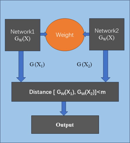
Here, N represents the number of samples, E_w denotes the Euclidean distance between the outputs of the Siamese network, and E_w = |X₁ − X₂|², where X₁ and X₂ are input data pairs. The input sample is represented as ((X₁, X₂), Y), where Y takes a value of 1 or 0. If the prediction model indicates that the inputs are similar, Y is assigned as 1; otherwise, it is assigned as 0. m represents the threshold value for dissimilar distances, where the distance between two dissimilar samples falls within [0, m]. When the distance exceeds m, the dissimilarity between the two samples is considered as 0.

Based on the data collected by the Micro-Hyperspace hyperspectral imager, we used ENVI software to pre-process the original hyperspectral image by logarithmic residual atmospheric correction, Fourier transform noise removal, Fourier image enhancement, etc. The ROI of 100 × 100 pixels about healthy travertine, black travertine, algal erosion travertine, and bare soil was cropped in the image, and the average spectral curve of ROI was extracted as the reflectivity curve.

2.2.2. Spectral feature extraction method

Since high dimensions and slow data processing characterize hyperspectral data, we chose the PCA dimensionality reduction method with the feature that ‘each principal component is orthogonal, which can eliminate the mutual influence between the original data’ to reduce the dimensionality of the pre-processed data. The dimensionality reduction of PCA uses fewer principal components to represent the internal structure of the original multiple variable indicators and lower dimensions to reflect the overall structure of the data. It is generally believed that the variance accumulation rate of the principal components of the dimensionality reduction data reaches 80%, and the dimensionality reduction data can retain the differentiation of the original data to a large extent (Marsboom et al. 2018; Booker et al. 2022). It is a method of unsupervised learning.

In this study, travertine-sensitive bands are extracted by combining the identification of bands of different minerals and the band data that can reflect the peaks and troughs of the travertine spectral curve and then screening. The spectral identification of bands of different mineral types (Yu et al. 2023) are shown in Table 3. Finally, the PCA dimensionality reduction method and the travertine-sensitive band extraction method were combined to form the travertine spectral feature extraction method.

Table 3. Identification range of different mineral bands (Yu et al. 2023).

Band type	Band range (nm)	Mineral types can be identified
Visible light – near infrared	400–1200	Hematite, specula rite
Short wave infrared	1300–1.82	Hydroxide, carbonate, sulfate
	1.47–1.82	Carbonate: alum stone
	2.16–2.24	Al–OH minerals: Muscovite, kaolinite, montmorillonite
	2.24–2.30	Fe–OH mineral: potassium iron sail, lithium soapstone
	2.26–2.30	Calcite, dolomite, magnesite
	2.30–2.40	Mg–OH minerals: chlorite, talc, epidote

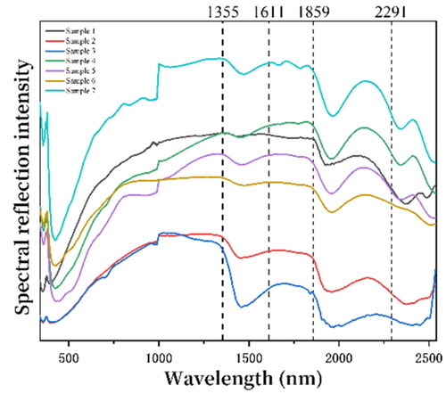
The process of extracting sensitive bands for travertine is as follows. Taking the hyperspectral spectra of a specific travertine sample in Figure 7 as an example, considering that the main components of Huanglong travertine are carbonates and sulfates, the feature reflectance within the range of 1300–1820 nm was extracted. Specifically, the reflectance of the peak and valley within the range of 1355–1859 nm was extracted. However, because the spectral range of imaging spectrometers is generally 300–1000 nm, the reflectance of the peak and valley within this range was also extracted. In order to reduce data processing time, the reflectance above the 1820 nm band was not extracted, including the reflectance data within the range of 1859–2291 nm. These data were already compressed in a lower-dimensional form in the dataset during the PCA dimension reduction stage.

Figure 7. Sensitive band extraction example.

2.2.3. Establishment of PSO-BPNN recognition model

BPNN is a multilayer pre-error feedback neural network under the error backpropagation algorithm. It comprises an input, output, and multiple hidden layers. Each hidden layer consists of several nodes representing neurons, with weights connecting the nodes of adjacent layers. The nodes within each layer are interconnected, but there is no association between nodes within the same layer (Yang et al. 2021; Sun 2022). The fundamental principle is illustrated in the bottom left sub-diagram of Figure 8. In this diagram, X₁ and X₂ are nodes of the input layer, Q₁, Q₂, and Q₃ are nodes of the hidden layer, and u represents the nodes of the output layer. W₁₁, W₁₂, W₁₃, W₂₁, W₂₂, and W₂₃ denote the initial weights connecting the input layer to the hidden layer, β represents the threshold of the hidden layer, β₁, β₂, and β₃ denote the initial thresholds, V represents the weight connecting the hidden layer to the output layer, λ represents the output layer threshold, y‘ represents the output value, and h represents the activation function, employing the LOGSIG function (Figure 9).

Figure 8. PSO-BPNN model establishment diagram.

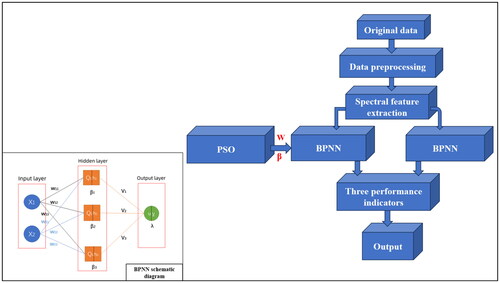
Figure 9. LOGSIG function image.

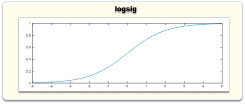
The LOGSIG function is a logarithmic function of type S, and its formula is as follows: (2) $$\mathit{\text{Logsig}}\left(x\right)=\frac{1}{1+e^{-x}}$$(2)

X can be any input value or visible function image. The function’s output value is between (0,1), the messy input value is mapped between 0 and 1, and the introduction of the nonlinear activation function can improve the network’s ability for nonlinear fitting.

Despite being a self-feedback model that achieves self-improvement by presetting the error, the initial weights (W) and threshold (β) from the input layer to the hidden layer of BPNN are set randomly. This study uses Particle Swarm Algorithm (PSO) to optimize the settings of W and β of the BPNN. Inspired by the behavioral research of birds feeding in flocks, the PSO leverages information sharing among individuals in the flock to evolve from disorder to order in the problem-solution space and obtain the optimal positions of individuals and the flock (Wang et al. 2018; Jain et al. 2022). One crucial step in this algorithm is to update the velocity and position of each particle, for which the following formulas (3) and (4) are employed for particle velocity and position updating. (3) $$v_{\mathit{\text{id}}}^{k+1}=w{v}_{\mathit{\text{id}}}^k+c_1{r}_1\left(p_{\mathit{\text{id}},\mathit{\text{pbest}}}^k-x_{\mathit{\text{id}}}^k\right)+c_2{r}_2\left(p_{d,\mathit{\text{gbest}}}^k-x_{\mathit{\text{id}}}^k\right)$$(3) (4) $$x_{\mathit{\text{id}}}^{k+1}=x_{\mathit{\text{id}}}^k+v_{\mathit{\text{id}}}^{k+1}$$(4) $v_{\mathit{\text{id}}}^k$ is the velocity vector of particle i in the dth dimension in the kth iteration; $x_{\mathit{\text{id}}}^k$ is the position vector of particle i in the dth dimension in the kth iteration; $p_{\mathit{\text{id}},\mathit{\text{pbest}}}^k$ is the historical optimal position of particle i in the dth dimension in the kth iteration; $p_{d,\mathit{\text{gbest}}}^k$ is the historical optimal position of the population in the dth dimension in the kth iteration; c₁ is a learning factor; c₂ is a group learning factor; w is an inertia factor value is non-negative, the larger the value, the stronger the global optimization search ability, the weaker the local optimization search ability; r1 and r2 are random numbers in the interval [0,1] to increase the randomness of the search. The application of Particle Swarm Optimization (PSO) to Back Propagation Neural Networks (BPNN) involves treating the input of all sample data as a group, with each sample being an individual. Calculating individual and global adaptation values, individual extreme values, and group extreme values is performed. The global optimal particle position is obtained after a certain number of iterations (determined based on optimizing the worldwide adaptation value). The individual and population extreme values are then assigned to the parameters W and β of the BPNN to enhance its prediction performance.

For this study, a three-layer structure was selected for the BPNN classifier, consisting of an input layer, a hidden layer, and an output layer. The number of nodes in the input layer was set to 17, the number of nodes in the hidden layer was 6, and the number of nodes in the output layer was 4, based on the feature dataset. The target error was set as the root-mean-square error (MSE) with a value of 1e-5.

2.2.4. Method for evaluating model performance

The confusion matrix is a square n*n representing the accuracy evaluation format. This study used MATLAB programming to obtain the confusion matrices for each result. It is utilized to derive the values of TP, TN, FP, and FN (Barranco-Chamorro and Carrillo-García 2021; Krstinić et al. 2023). TP refers to actual and correctly classified instances, TN represents valid instances erroneously categorized as false, FP denotes faulty models incorrectly classified as accurate, and FN indicates false and correctly classified instances.

The formulas (5)–(9) below are employed to calculate three performance metrics: F1 score, kappa coefficient, and overall accuracy (OA). A model performs better when the F1 score and kappa coefficient are closer to 1. In contrast, a version closer to 0 indicates poorer model performance. Values above 0.5 are typically deemed significant, meaning good model performance (Heydarian et al. 2022; Wang et al. 2022). Precision and Recall are crucial indicators used in the computation of the F1 score. (5) $$\mathit{\text{Precision}}=\frac{\mathit{\text{TP}}}{\mathit{\text{TP}}+\mathit{\text{FP}}}$$(5) (6) $$\mathit{\text{Recall}}=\frac{\mathit{\text{TP}}}{\mathit{\text{TP}}+\mathit{\text{FN}}}$$(6) (7) $$\mathit{\text{OA}}=\mathit{\text{po}}=\frac{\mathit{\text{TP}}+\mathit{\text{TN}}}{\mathit{\text{TP}}+\mathit{\text{TN}}+\mathit{\text{FP}}+\mathit{\text{FN}}}$$(7) (8) $$F1=2\times \frac{\mathit{\text{Pecision}}\mathrm{\hspace{0.17em}*\hspace{0.17em}}\mathit{\text{Recall}}}{\mathit{\text{Precision}}+\mathit{\text{Recall}}}=\frac{\mathit{\text{TP}}}{\mathit{\text{TP}}+\frac{\mathit{\text{FN}}+\mathit{\text{FP}}}{2}}$$(8) (9) $$\mathit{\text{kappa}}=\frac{\mathit{\text{po}}-\frac{\left(\mathit{\text{TP}}+\mathit{\text{TN}}+\mathit{\text{FP}}+\mathit{\text{FN}}\right)\mathrm{\hspace{0.17em}*\hspace{0.17em}}\mathit{\text{po}}\mathrm{\hspace{0.17em}*\hspace{0.17em}}\left(\mathit{\text{TP}}+\mathit{\text{FP}}\right)+\left(\mathit{\text{FP}}+\mathit{\text{TN}}\right)\mathrm{\hspace{0.17em}*\hspace{0.17em}}(\mathit{\text{FN}}+\mathit{\text{TN}})}{{(\mathit{\text{TP}}+\mathit{\text{TN}}+\mathit{\text{FP}}+\mathit{\text{FN}})}^2}}{1-\frac{\left(\mathit{\text{TP}}+\mathit{\text{TN}}+\mathit{\text{FP}}+\mathit{\text{FN}}\right)\mathrm{\hspace{0.17em}*\hspace{0.17em}}\mathit{\text{po}}\mathrm{\hspace{0.17em}*\hspace{0.17em}}\left(\mathit{\text{TP}}+\mathit{\text{FP}}\right)+\left(\mathit{\text{FP}}+\mathit{\text{TN}}\right)\mathrm{\hspace{0.17em}*\hspace{0.17em}}(\mathit{\text{FN}}+\mathit{\text{TN}})}{{(\mathit{\text{TP}}+\mathit{\text{TN}}+\mathrm{F}P+\mathit{\text{FN}})}^2}}$$(9)

3. Results and discussion

3.1. Results and discussion of spectral feature extraction

The spectral reflectance data collected by PSR-2500 for three travertine and bare soil states were subjected to PCA dimensionality reduction. In this paper, the variance share and cumulative variance share of the principal components after dimensionality reduction are analyzed, and it is found that the variance share of each of the first three principal components is 0.58, 0.3, and 0.1, respectively, and the variance share of the fourth principal component is lower than the decile value. Usually, the cumulative variance of the principal components reaches 80% of the principal components to meet the requirements of the dimensionality reduction process and retain most of the values of the difference between the differences. However, the cumulative variance of the first two principal components can reach 88%. However, to ensure the retention of more data to distinguish between the differences in the values of the third principal component, the total cumulative variance reached 98%. The original data was then reduced to three dimensions based on the product of the eigenvectors corresponding to the first three principal components and the original data matrix (Table 4).

Table 4. Interpretation of variance of PCA principal components.

Total variance interpretation
Principal components	Eigenvalue	Variance ratio	Cumulative variance
1	448.92	0.58	0.58
2	230.98	0.30	0.88
3	79.58	0.10	0.98

The downscaling of spectral reflectance, although it can retain most of the numerical differences of the travertine classification data, will still be part of the information available for discrimination is missing, so the sensitive waveband data of travertine and bare earth are extracted as the feature data supplement. The sensitive bands of travertine and bare soil were obtained through the sensitive band extraction method, as shown in Table 5. This paper found that the extracted characteristic bands of three kinds of travertine and bare soil were mainly distributed in the 400–1800 nm band, and the sensitive bands of healthy travertine mainly appeared in the range of the visible band (400–780 nm); the sensitive bands of darkened travertine were found in the visible and infrared bands; the sensitive bands of algal erosion travertine The sensitive bands for algal erosion travertine blooms were more frequent in the green and yellow bands; the sensitive bands for bare soil were very similar to those for healthy travertine blooms, mainly in the visible and near-infrared bands. It can be seen that the reaction of travertine is more robust in the visible light band.

Table 5. Spectrally sensitive bands.

Variety	Wavelength(nm)
Healthy travertine	420.2, 460.2, 522, 542.8, 596.9, 615.6, 662.1, 658, 716.8, 727.5, 834.9, 1300.8, 1319.9, 1402.3
Blackened travertine	423.4, 638.3, 710.1, 755, 834.9, 1307.2, 1326.2, 1408.6, 427.6, 1522.1, 1628.8, 1647.6, 1710.2
Algal erosion of travertine	400, 526.5, 542.8, 556.1, 570.7, 591.1, 685.6, 744.6, 870, 995.6, 1547.3, 1635.1, 1653.9, 1716.4
Bare soil	404.7, 437.2, 486, 510.1, 536.9, 575.1, 608.4, 641.1, 667.7, 740.6, 856.1, 1115.8, 1256.3, 1345.3

3.2. Classification of BPNN and PSO-BPNN

The dimensionality-reduced data and the sensitive band reflectance data form this study’s feature dataset. The feature dataset is randomly divided into a training set and a test set according to the ratio of 7:3 and then inputted into BPNN and PSO-BPNN to identify healthy travertine blooms, darkened travertine blooms, algal erosion travertine blooms, and bare ground, respectively. F1-score, kappa coefficient, and OA evaluation metrics were used to compare the performance of BPNN classifiers and PSO-BPNN classifiers.

The confusion matrix in Figure 10 shows the correct and incorrect rates of prediction for various classes in the real and predicted class labels for species 1–4, which are healthy travertine, blackened travertine, algal erosion travertine, and bare soil, respectively. (a) The confusion matrix of Figure. The correct prediction rate for species 1 of the real class is 79.3%, for species 2 is 82.6%, for species 3 is 68.2%, and for species 4 is 77.3%. (b) The correct prediction rates for the four categories of the real class in the figure are, respectively, 75, 70, 80, and 80%, and (c) The correct prediction rates for the four categories of the real class in the figure are, respectively, 89.7, 91.3, 86.4, and 90.0%. (d) The correct prediction rates for the four categories in the true category in the figure are 91.7, 90, 90, and 90%, respectively.

Figure 10. (a) Confusion matrix illustrating the classification results for the BPNN training set; (b) confusion matrix illustrating the classification results for the BPNN test set; (c) confusion matrix depicting the classification results for the PSO-BPNN training set; (d) confusion matrix illustrating the classification results for the PSO-BPNN test set.

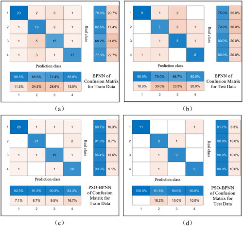
And in the predictive category, (a) the correct prediction rate for Category 1 in the figure is 88.5, 65.5% for category 2, 71.4% for category 3, and 85% for category 4. (b) The correct prediction rates for the four categories in the figure are, respectively, 90, 70, 66.7, and 80%, (c) The correct prediction rates for the four categories in the figure are, respectively, 92.9, 91.3, 90.5, and 83.3%, and (d) The correct prediction rates for the four categories in the figure are, respectively, 100, 81.8, 90, and 90%.

The classification results of the predicted classes better reflect the effect of the classification model than the real classes. From the comparison of the results of the predicted classes in the training and test sets of the BPNN and PSO-BPNN models, the prediction correctness rate of the PSO-BPNN model is generally higher than that of the BPNN. However, not all of them are like this; for example, the correctness rate of the predicted classes of category 4 in the training set of the BPNN model is higher than the correctness rate of the predicted classes of category 4 in the training set of the PSO- BPNN model. For example, in the BPNN training set, the correctness of the prediction class of category 4 in the training set of the BPNN model is higher than that of the PSO-. In order to compare the classification performance of BPNN and PSO-BPNN models more comprehensively, this paper derives the TP, TN, FP, and FN values of the prediction results of the four categories based on the principle of the four-category confusion matrix. It calculates the F1-score, kappa coefficient, and OA values, which are organized as shown in Table 6. The performance differences of the models are explored by comparing the three performance metrics of the four categories.

Table 6. Model performance index.

Model type	DS	Recognition category	TP	TN	FP	FN	F1-score	Kappa	OA
BPNN	Training set	Healthy travertine	23	64	3	6	0.84	0.77	0.79
		Black travertine	19	63	10	4	0.73	0.63	0.83
		Algal erosion of travertine	15	68	6	7	0.70	0.61	0.68
		Bare soil	17	71	3	5	0.81	0.76	0.77
	Test set	Healthy travertine	9	29	1	3	0.82	0.75	0.75
		Black travertine	7	29	3	3	0.70	0.61	0.70
		Algal erosion of travertine	8	28	4	2	0.73	0.63	0.80
		Bare soil	8	30	2	2	0.80	0.74	0.80
PSO-BPNN	Training set	Healthy travertine	26	65	2	3	0.91	0.88	0.90
		Black travertine	21	71	2	2	0.91	0.89	0.91
		Algal erosion of travertine	19	72	2	3	0.88	0.85	0.86
		Bare soil	20	70	4	2	0.86	0.83	0.91
	Test set	Healthy travertine	11	30	0	1	0.96	0.94	0.92
		Black travertine	9	30	2	1	0.86	0.81	0.90
		Algal erosion of travertine	9	31	1	1	0.90	0.87	0.90
		Bare soil	9	31	1	1	0.90	0.87	0.90

In Table 6, all the values of the F1-score and kappa coefficient performance indexes in the BPNN model are observed. It is found that all the values of these two indexes are above 0.5. For the classification model, these two indexes usually reach a value above 0.5, indicating that the model’s performance is already within a good range, which may be reflected from the side of the data preprocessing effect. This may reflect that the data’s preprocessing effect is relatively good.

The classification results of the predicted classes better reflect the effect of the classification model than the real classes. A careful comparison of the three performance index values between BPNN and PSO-BPNN reveals that the performance of PSO-BPNN is better than that of BPNN in classifying all four categories. The extent of PSO's performance enhancement of BPNN can be seen in the fact that the PSO-BPNN model’s three indexes of the algal encroachment of travertine blooms in the training set are 0.88, 0.85, and 0.86, respectively, compared with that of the BPNN model in the training set. The three performance metrics of the model on algal erosion calcium bloom in the training set are improved by 0.18, 0.24, and 0.18, respectively, which can reflect that the PSO algorithm’s method of finding the globally optimal weights and thresholds for the BPNN from the model’s input feature set has a significant effect on the performance enhancement of the BPNN. By comparing the classification results of the training and test sets of the PSO-BPNN model, it is found that its performance is not stable. For example, the classification effect of the blackened calvarium in the training set is slightly worse than in the test set although the same problem exists in the BPNN model, which may be due to the model’s parameter values depending on experience, it also exists in PSO-BPNN, which indicates that the PSO algorithm has some shortcomings in some aspects.

3.3. The recognition model applied to hyperspectral images of calvary

In order to further verify whether the practical application of the recognition model in remote sensing images in this paper is excellent, experiments are carried out using data collected in the field by the Micro-Hyperspace hyperspectral imager. The average reflectance data of 178 cropped images acquired from hyperspectral remote sensing images are used as the dataset for this validation, and the dataset is preprocessed with Savitzky-Golay and MSC. After the feature subset was produced, the feature subset was randomly divided into a training set and a test set in the ratio of 7:3 and input into the PSO-BPNN recognition model, and the performance index was analyzed to evaluate the effect of the model. The processing results of hyperspectral image data are shown in Figure 11.

Figure 11. (a) And (b) display sample hyperspectral images; (c), (d), (e), and (f) represent the regions of interest (ROI) depicting RGB images of black travertine, bare soil, healthy travertine, and algal erosion of travertine, respectively; (g) and (h) represent the confusion matrices illustrating the classification results of the training set and the test set, respectively.

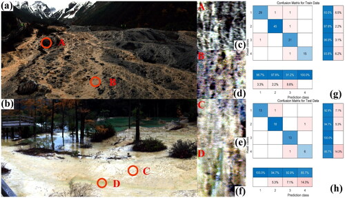
The spectral band range of data acquired by the Micro-Hyperspace hyperspectral imager is similar to that of active hyperspectral satellites, and the classification results of analyzing the data from this image as the experimental object of the model can provide a certain reference for the application of data from active hyperspectral satellites. Analyzing the results of the confusion matrices of the training and test sets in Figure 8, the prediction accuracies of the four categories in the confusion matrix of the training set are 93.5, 97.8, 96.9, and 93.8%, respectively, under the label of the real category, and the prediction accuracies of the four categories under the label of the predicted category are 96.7, 97.8, 91.2, and 100%, respectively; in the confusion matrix of the test set, the predictions of the four categories under the label of the real category are 96.7, 97.8, 91.2, and 100%. Class label, the prediction accuracy of the four categories is 92.9, 94.7, 100, 85.78%, and under the prediction class label, the accuracy of the four categories is 100, 94.7, 92.9, and 85.7%, respectively. It can be seen that the accuracy of the classification results performs relatively well both in the training set and the test set. The confusion matrix is calculated to yield the three performance index values shown in the Table 7.

Table 7. Performance indicators of model validation set.

DS	Recognition category	TP	TN	FP	FN	F1-score	Kappa	OA
Training set	Healthy travertine	29	93	1	2	0.96	0.94	0.98
	Black travertine	45	78	1	1	0.98	0.97	0.98
	Algal erosion of travertine	31	90	3	1	0.94	0.92	0.97
	Bare soil	15	109	0	1	0.97	0.96	0.99
Test set	Healthy travertine	13	39	0	1	0.96	0.95	0.98
	Black travertine	18	33	1	1	0.95	0.92	0.96
	Algal erosion of travertine	13	39	1	0	0.96	0.95	0.98
	Bare soil	6	45	1	1	0.86	0.84	0.96

Analyzing the values of the three performance metrics in Table 7, the values of the four categories of performance metrics are above 0.8 in both the training set and the test set, which shows that the model obtained from the training of the PSR-2500 spectrometer data with a broader range of wavebands has a good effect on classifying the spectral data in the range of the wavebands of 400–1000. Even though this PSO-BPNN model adds learning from the Micro-Hyperspace hyperspectral imager data training set, there is still a similar situation to that in 3.2, i.e. the values of the three performance metrics of blackened Calcium Wahoo and bare earth in the training set are more significant than that in the test set. The values of the classification performance metrics of bare earth have a significant difference between the training set and the test set, with a difference in the F1-score of 0.11 and a Kappa difference of 0.8. After analyzing, the general generation of this situation is related to the model’s structure and the data’s preprocessing.

4. Conclusion

In this paper, spectral data were used to classify and recognize the four categories of healthy travertine bloom, blackened travertine bloom, algal erosion travertine bloom, and bare soil, and a series of correlation processing was carried out for the spectral data before inputting into the improved BPNN for classification and recognition. In terms of feature extraction, this paper investigates how to maximize the retention of the different information of different states of travertine and bare soil and adopts a combination of PCA dimensionality reduction and sensitive band extraction; after the PCA dimensionality reduction, the first three principal components are selected as the basis for dimensionality reduction according to the proportion of the variance of the principal components and the cumulative proportion of the variance of the principal components; the extraction of the sensitive bands is based on the combination of the spectral identification of band of the minerals in travertine with the spectral identification of band of the actual different states of travertine. Sensitive bands are extracted by combining the spectral identification of bands of the minerals in the travertine and the response bands of different states of the actual travertine to the spectra. In this process, it is found that the three states of the travertine are more sensitive to the visible band and the near-infrared band of the light.

In the process of analyzing and comparing the BPNN and PSO-BPNN models, the confusion matrix of the classification results and the values of the classification performance indexes of the four categories show that the optimization of the initial weights and thresholds provided by the PSO algorithm for the BPNN can effectively improve the classification performance of the BPNN for the four categories. However, there is still a need to further improve the stability of the model. In this paper, the spectral data acquired by Micro-Hyperspace hyperspectral imager is used to verify whether the model trained by PSR-2500 spectrometer data can provide a reference for active satellites in the identification of Travertine to make experiments, and from the classification results, the model has good results in the identification of different states of Travertine and bare soil data by Micro-Hyperspace hyperspectral imager, but the model classification also appears to have good results. The results show that the model effectively recognizes the different states of travertine and bare soil data from the Micro-Hyperspace hyperspectral imager. However, the model also shows unstable classification performance. The authors expect that the unstable classification performance of the model can be solved by increasing the data training volume of the model, analyzing the interrelationships of the feature dataset, and further optimizing the classifier.

In addition, the band data of the Micro-Hyperspace hyperspectral imager is very similar to that of existing hyperspectral satellites. The purpose of using the PSR-2500 ground object spectrometer and Micro-Hyperspace Hyperspectral imager data is to test whether the broader spectral band data model of the PSR-2500 Ground object spectrometer can be applied to the Micro-Hyperspace Hyperspectral imager data. To explore whether this method can provide a reference for hyperspectral satellites in service and for future imaging spectrometers with wider bands. From the experiment of this paper, the method in this paper can help with the above problems.

Disclosure statement

No potential conflict of interest was reported by the author(s).

Additional information

Funding

His work was supported by the Southwest University of Science and Technology under Grante 21ZX7106 and 22ZX7171, Science and Technology Department of Sichuan Province under Grante 23KPZP0129, and National Natural Science Foundation-Regional Innovation and Development Joint Fund, U21A2016.

References

- Brown AJ. 2006. Spectral curve fitting for automatic hyperspectral data analysis. IEEE Trans Geosci Remot Sens. 44(6):1601–1608. doi: 10.1109/TGRS.2006.870435.
- Brown AJ, Hook SJ, Baldridge AM, Crowley JK, Bridges NT, Thomson BJ, Marion GM, de Souza Filho CR, Bishop JL. 2010. Hydrothermal formation of clay-carbonate alteration assemblages in the Nili Fossae region of Mars. Earth Planet Sci Lett. 297(1–2):174–182. doi: 10.1016/j.epsl.2010.06.018.
- Barranco-Chamorro I, Carrillo-García RM. 2021. Techniques to deal with off-diagonal elements in confusion matrices. Mathematics. 9(24):3233. doi: 10.3390/math9243233.
- Booker NK, Knights P, Gates JD, Clegg RE. 2022. Applying principal component analysis (PCA) to the selection of forensic analysis methodologies. Eng Fail Anal. 132:105937. doi: 10.1016/j.engfailanal.2021.105937.
- Cen Y, Huang Y, Hu S, Zhang L, Zhang J. 2022. Early detection of bacterial wilt in tomato with portable hyperspectral spectrometer. Remote Sens. 14(12):2882. doi: 10.3390/rs14122882.
- Cui S, Zhou K, Ding R, Jiang G. 2019. Estimation of copper concentration of rocks using hyperspectral technology. Front Earth Sci. 13(3):563–574. doi: 10.1007/s11707-019-0753-0.
- Diago-Cisneros L. 2022. Corrigendum to “unitarity and symmetries of the multicomponent scattering matrix. Ann Phys. 437:168729. doi: 10.1016/j.aop.2020.168255.
- Galdames FJ, Perez CA, Estévez PA, Adams M. 2022. Rock lithological instance classification by hyperspectral images using dimensionality reduction and deep learning. Chemomet Intell Lab Syst. 224:104538. doi: 10.1016/j.chemolab.2022.104538.
- Gao P, Zhang H, Yu J, Lin J, Wang X, Yang M, Kong F. 2021. Secure cloud-aided object recognition on hyperspectral remote sensing images. EEE Internet Things J. 8(5):3287–3299.
- Heydarian M, Doyle TE, Samavi R. 2022. MLCM: multi-label confusion matrix. IEEE Access. 10:19083–19095. doi: 10.1109/ACCESS.2022.3151048.
- Huang D, Yang M, Duan J, Yu S, Liu Z. 2023. Siamese network tracking based on feature enhancement. IEEE Access. 11:37705–3713. doi: 10.1109/ACCESS.2023.3266264.
- Jain M, Saihjpal V, Singh N, Singh SB. 2022. An overview of variants and advancements of PSO algorithm. Appl Sci. 12(17):8392. doi: 10.3390/app12178392.
- Jiang Z, Dai Q, Dong F, Zhang Q, Dang Z, Wang Z, Liu F. 2021. Research progress and prospect of travertine karst landscape at home and abroad. Karst China. 40(01):4–10.
- Jiang Q, Wu G, Tian C, Li N, Yang H, Bai Y, Zhang B. 2021. Hyperspectral imaging for early identification of strawberry leaves diseases with machine learning and spectral fingerprint features. Infrared Phy Technol. 118:103898. doi: 10.1016/j.infrared.2021.103898.
- Krstinić D, Šerić L, Slapničar I. 2023. Comments on “MLCM: multi-label confusion matrix. IEEE Access. 11:40692–40697. doi: 10.1109/ACCESS.2023.3267672.
- Li G, Dong F, Dai Q, Dang Z, Zhao Y. 2018. Comparative study on the determination methods of organic carbon in Huanglong travertine. J Petromineral. 37(01):152–160.
- Lin F, Guo S, Tan C, Zhou X, Zhang D. 2020. Identification of rice sheath blight through spectral responses using hyperspectral images. Sensors. 20(21):6243. doi: 10.3390/s20216243.
- Liu F, Wang F, Wang X, Liao G, Zhang Z, Yang Y, Jiao Y. 2022. Rapeseed variety recognition based on hyperspectral feature fusion. Agronomy. 12(10):2350. doi: 10.3390/agronomy12102350.
- Liu X, Zhang Q, Sun D, Tang S, Tian C, Huang H, Zhou Y, Xiong Y, Liang X, Fan J, et al. 2023. Dynamic characteristics of water environment and analysis of travertine deposition capacity in Huanglong Core scenic area. Karst in China. 42(6):1149–1160.
- Liu W, Zeng S, Wu G, Li H, Chen F. 2021. Rice seed purity identification technology using hyperspectral image with LASSO logistic regression model. Sensors. 21(13):4384. doi: 10.3390/s21134384.
- Marsboom C, Vrebos D, Staes J, Meire P. 2018. Using dimension reduction PCA to identify ecosystem service bundles. Ecol Indic. 87:209–260. doi: 10.1016/j.ecolind.2017.10.049.
- Qiao X, Liu X, Wang F, Sun Z, Yang L, Pu X, Huang Y, Liu S, Qian W. 2022. A method of invasive alien plant identification based on hyperspectral images. Agronomy.12(11):2825. doi: 10.3390/agronomy12112825.
- Qiao X, Xiao N, Du J, Tang Y, Xiao W, Zhen Y, Zhang M. 2022. Research progress and prospect of travertine landscape in the core scenic area of Jiuzhaigou World Natural Heritage. Earth Environ. 50(2):202–218.
- Rao H, Dong F, Liu M, An D, Dai Q, Li Q, Zhang Q, Liu X, Liu Z, Zhang Y. 2023. Structural changes and driving factors of chilling diatom community in algal mat in Huanglong Scenic Area. Karst in China. 42(3):482–494.
- Ricketts JW, Ma L, Wagler AE, Garcia VH. 2019. Global travertine deposition modulated by oscillations in climate. J Quat Sci. 34(7):558–568. doi: 10.1002/jqs.3144.
- Román-Gallego J-Á, Pérez-Delgado M-L, San Gregorio SV. 2022. Convolutional neural networks used to date photographs. Electronics. 11(2):227. doi: 10.3390/electronics11020227.
- Romo-Cárdenas G, Avilés-Rodríguez GJ, Sánchez-López JdD, Cosío-León M, Luque PA, Gómez-Gutiérrez CM, Nieto-Hipólito JI, Vázquez-Briseño M, Navarro-Cota CX. 2018. Nyquist-Shannon theorem application for Savitzky-Golay smoothing window size parameter determination in bio-optical signals. Results Phys. 11:17–22. doi: 10.1016/j.rinp.2018.08.033.
- Sun H. 2022. Prediction of building energy consumption based on BP neural network. Wireless Commun Mobile Comput. 2022:1–10.
- Sun Y, Ding S, Zhang Z, Jia W. 2021. An improved grid search algorithm to optimize SVR for prediction. Soft Comput. 25(7):5633–5644. doi: 10.1007/s00500-020-05560-w.
- Sun Y, Qian X, Liu Y, Wang J, Lv Q, Yuan M. 2021. Identification of typical solid hazardous chemicals based on hyperspectral imaging. Remote Sens. 13(13):2608. doi: 10.3390/rs13132608.
- Wang Z, Fu X, Du K, Liu J, Che X. 2022. Typical geographic object detection in map images supported by deep learning. Bullet Survey Map. 11:74–78.
- Wang D, Tan D, Liu L. 2018. Particle swarm optimization algorithm: an overview. Soft Comput. 22(2):387–408. doi: 10.1007/s00500-016-2474-6.
- Wang J, Wang W, Cheng Y, Zhang Z, Wang S, Zhou K, Li P. 2021. Estimation of rock Fe content based on hyperspectral indices. J Arid Land. 13(12):1287–1298. doi: 10.1007/s40333-021-0110-5.
- Xu D, Zhang D, Shi D, Luan Z. 2020. Automatic extraction of open water using imagery of landsat series. Water. 12(7):1928. doi: 10.3390/w12071928.
- Yadav D, Arora MK, Tiwari KC, Ghosh JK. 2019. Identification of most useful spectral ranges in improvement of target detection using hyperspectral data. Egypt J Remot Sens Space Sci. 22(3):347–357. doi: 10.1016/j.ejrs.2018.04.002.
- Yang S, Luo L, Tan B. 2021. Research on sports performance prediction based on BP neural network. Mob Inform Syst. 2021:1–8.
- Yu Z, Fang H, Zhangjin Q, Mi C, Feng X, He Y. 2021. Hyperspectral imaging technology combined with deep learning for hybrid okra seed identification. Biosyst Eng. 212:46–61. doi: 10.1016/j.biosystemseng.2021.09.010.
- Yu Q, Shao Y, et al. 2023. Study on lithology hyperspectral identification and model accuracy of carbonate rock. Laser J. 44(01):27–31.
- Zhang H, Xing W, Yang Y, Li Y, Yuan D. 2023. SiamST: Siamese network with spatio-temporal awareness for object tracking. Inf Sci. 634:122–139. doi: 10.1016/j.ins.2023.03.083.
- Zhao S, Zhang B, Philip Chen CL. 2019. Joint deep convolutional feature representation for hyperspectral palmprint recognition. Inf Sci. 489:167–181. doi: 10.1016/j.ins.2019.03.027.