Partitioning building groups at multiple scales based on image segmentation

Abstract

The partitioning of building groups is a prerequisite for map generalization. Existing methods center on the spatial relationships between individual buildings, neglecting the interrelations among building groups. As such, these methods prove suitable only for identifying building groups at a single scale. In this research, we introduce a novel methodology for partitioning building groups across multiple scales by employing image segmentation, thus enabling the simultaneous recognition of building groups of all scales within a recognition unit. First, image segmentation and merging approaches were employed to extract merged image regions, representing the spatial relationships of building groups. Then, the process commenced with the construction of a graphical representation encompassing buildings and merged regions, wherein the edges were assigned weights indicative of the closeness between groups of buildings. Finally, the graph underwent a progressive segmentation process, and a scale set of building groups was established. Based on the experimental findings, the proposed approach can proficiently partition building groups across various scales. This is demonstrated by the accuracy rate surpassing 90% in the complex experimental area. One can effortlessly derive building groups from the scale set by using a predetermined scale parameter. These findings may serve as a fundamental basis for the implementation of multiscale map generalization and the linkage updating of multiscale spatial data.

Keywords:

• Partition of building groups
• image segmentation
• multiple scales
• map generalization

1. Introduction

As significant places for human habitation and productivity, buildings are ubiquitous elements within urban landscapes. In the field of cartography, a crucial aspect of buildings is that they are generalizable at a certain range of scales. The generalized buildings are usually derived from various building groups at different scales. These groups are formed by the arrangement or combination of buildings, which is determined by the spatial relationships between buildings, such as distance, direction, and size (Du et al. 2016). In terms of their arrangement, building groups exhibit various patterns, such as linear, curvilinear, and grid patterns. The partitioning of building groups at multiple scales aims to partition individual buildings into diverse clusters at different scales, based on their spatial configuration, geometric attributes, and semantic features. Partitioning building groups in topographic maps plays a vital role in the analysis and modeling of geographic spaces. It allows for the generalization of recognized building groups while preserving the spatial configuration of the buildings in a scene (Mackaness et al. 2014). It hence plays an essential role in a wide variety of downstream applications, such as map generalization (i.e. the procedure that utilizes transformation operations to solve spatial conflicts of entities and derive smaller-scale maps from large-scale-maps) and semantic classification of urban structures and functions (Du et al. 2015; Niu et al. 2017).

In the field of cartography, the prevailing building group partitioning approaches primarily revolve around ascertaining the feasibility of grouping two buildings. Specifically, buildings and their spatial relationships are represented through a connected graph, upon which segmentation can subsequently be performed. In the graph, vertices represent the buildings, and edges indicate the adjacency relationships between buildings. Edges are often weighted by the similarities of two adjacent buildings. Then, subgraphs (i.e. potential building groups) are extracted by cutting the edges of the graph. The criteria most commonly employed for assigning weights to the edges of graphs is often based on Euclidean distance, encompassing measures, such as nearest distance (Cetinkaya et al. 2015), average distance (Shuai et al. 2007), and visual distance (Ai and Guo 2007). Furthermore, the similarity in shape and size of buildings is frequently utilized to determine whether two buildings can be grouped together (Zhang et al. 2013; Yu et al. 2019; Sayidov et al. 2020). Evidently, the aforementioned studies only focus on the spatial relationship between buildings, overlooking the relationships between building groups.

Upon the removal of the edges of a graph, several connected subgraphs, which can be viewed as potential groups, may be obtained. Theoretically, determining whether a potential building group satisfies particular scale requirements can be considered as a classification problem. Numerous methodologies have been proposed to address such quandaries. For example, empirical criteria are often used to assess whether potential groups meet certain requirements. These approaches are commonly employed to recognize specific building groups, such as straight-line patterns (Nan et al. 2011; Delong et al. 2012; Wang et al. 2015). Such approaches necessitate the calibration of numerous empirical parameters. However, these parameters often vary across different recognition tasks and scales. With the capacity to derive numerous decision rules from samples, machine learning techniques can detect diverse building group patterns while minimizing the need for excessive human intervention. For example, Zhang et al. (2013) used the support vector machine algorithm to extract specific group patterns. In a study by Steiniger et al. (2010), a technique involving machine learning to decrease the search scope and to enhance the efficacy of map generalization was utilized. The efficacy of the random forest classifier in handling diverse scenarios has been demonstrated (Du et al. 2016). In a study by He et al. (2018), the authors utilized the random forest-based algorithm to recognize various kinds of building groups at the scale of 1:2000, including linear patterns, regular distribution patterns, L-type patterns, and high-density distribution patterns. Due to deep learning techniques being used in numerous research fields, Yan et al. (2019) tried to develop a graph convolutional neural network for the classification of building patterns using spatial vector data. Coincidentally, Knura (2023) demonstrated the application of deep learning methods for shape classification and template matching, which are pivotal for map generalization. Machine learning-based recognition methods can effectively identify single-scale building groups and minimize manual involvement. However, these methods require not only the gathering of substantial amounts of sample data but also constrain the identification of particular scales and categories of building groups. Moreover, these techniques are susceptible to regional differences and may have issues with data leakage, resulting in poor reproducibility (Kapoor and Narayanan 2023). Due to the variations in building distributions and the scale-dependent nature of group partitioning, the generalizability of machine learning-based methods remains limited, rendering them less useful in the partitioning of building groups across diverse scales and contexts. In summary, the prevailing methodologies are adept at partitioning building groups at a certain scale, which makes it difficult to apply them to generalize building representations across multiple scales.

Furthermore, the prevailing investigation has excessively prioritized the spatial relationships between adjacent individual buildings, neglecting the interconnections among building groups. This is because, in a topographic map that only includes building data, buildings are identified as objects while the vacant spaces between the buildings are perceived as background. However, these vacant spaces play an important role in group partitioning. In the real scene, these vacant spaces are pathways among building groups. Research has demonstrated that geographic phenomena, such as roads, pathways, or their characteristics, typically exhibit a reliance on scales (Li and Cai 2005). Stated differently, smaller geographic entities, such as roads, are more common than larger ones within a certain geographic space. Researchers have attempted to generalize buildings at various scales by using roads (Yan et al. 2008; Jiang et al. 2013; Zhang et al. 2023). However, the absence of detailed road data restricts these studies to only generalizing building blocks. Regrettably, most current road extraction methods primarily focus on recognizing urban roads (Xie et al. 2015; Deng et al. 2018). Furthermore, there is no universally accepted method that relies solely on vector data for partitioning building groups at different scales. In contrast, image segmentation permits the effortless achievement of multiscale, or even continuous scale, representations of images. Image segmentation refers to the procedure of segmenting an image into a series of continuous image merged regions that exhibit analogous attributes (Guigues et al. 2006). The region expression of an image involves using continuous merged regions obtained through image segmentation to accurately fit the entire image. During image segmentation, a series of merged regions can be derived according to different fitting errors. These continuous scale merged regions are vertically combined into a hierarchical structure, which forms the scale set of the image. Image segmentation technique has undergone extensive study and application (Hu et al. 2016, 2021). In particular, segmentation and merging technologies based on super pixels and watershed algorithms have reached a level of maturity (Hu et al. 2013). By employing image segmentation techniques, it may be feasible to extract image regions that represent the spatial relationships between building groups. Then, by progressively removing group relationships, building groups of varying scales can be obtained. This will be a brand-new attempt in the study of building group partitioning, solving the problem of building groups partitioning at various scales in map generalization in one go.

The remainder of this article is structured as follows: Section 2 presents the material introduction and provides a detailed description of the series of steps involved in the proposed methodology. The experiments, which include the implementation, partitioning results, and discussion, are detailed in Section 3. Finally, the conclusion is presented.

2. Materials and methodologies

2.1. Materials

Two images depicting building blocks and their corresponding vector data were selected for conducting the experiments (Figure 1). The image data consists of red, green, and blue spectral bands, with a resolution of 0.5 meters. The buildings in experimental area 1 are arranged in regular patterns (Figure 1(a)). The shapes of buildings are quite similar, resulting in a relatively simple group structure. Conversely, the arrangements of buildings within the experimental area 2 exhibited significant dissimilarity, featuring patterns of regular distribution, high-density clusters, and scattered layouts (Figure 1(b)). Visually, in both areas, all buildings can initially be partitioned into two major parts, and as the scale changes, the two parts are further partitioned into finer subgroups. Thus, these datasets provide ideal case studies that exemplify the partitioning of building groups across multiple scales.

Figure 1. Experimental data of two test areas comprising images, vector data of buildings, and road networks.

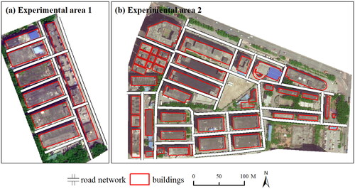
The vector data, scaled at 1:2000, was provided by the Guangzhou Urban Planning and Design Survey Research Institute in Guangdong Province, China. In our experiments, we utilized two types of road network data. The first type of road network data comprising the roads between building blocks was downloaded from a map website (i.e. AutoNavi map). These roads were used to partition all buildings into building blocks to amplify the efficacy of graph partitioning. The second type of road network data was manually extracted, serving as reference data for validating the recognition of building group relationships (Figure 1). These fine-scale roads are identifiable within building blocks but are not available on map websites. Building group reference data were obtained through manual recognition (Figure 2). Across all segmentations, a total of 22 building groups were identified.

Figure 2. Reference data derived from the manual recognition method.

2.2. Calculation of spatial relationships based on constrained Delaunay triangulation

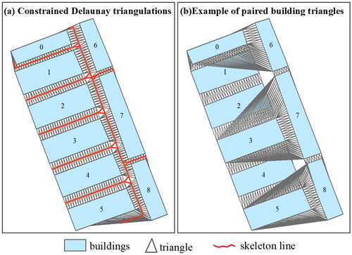
In this section, we outline methods for calculating the spatial relationships between individual buildings. First, buildings, road networks, and imagery are matched to each other to ensure consistency between the results obtained from image segmentation and merging with building data. Concurrently, the topographical map of buildings is partitioned into several building blocks using the road network. This partitioning reduces computational time for computing spatial relationships, thereby enhancing the efficacy of graph partitioning. Before creating constrained Delaunay triangulations (CDTs), building edges and surrounding roads are interpolated with points at specified intervals (e.g. 2 meters) to improve the accuracy of proximity detection. Two types of CDTs are then generated (Figure 3). The first type of CDTs is computed for all buildings within a block (Figure 3(a)), while another type of CDTs, known as paired building triangles, is computed only for each pair of adjacent buildings (Figure 3(b)). During this step, triangles connecting roads are excluded. Finally, spatial relationships between adjacent buildings are calculated based on the aforementioned CDTs, including proximity relationship (Equation 1(1) $$R=R(i,j)$$(1) ), skeleton line (Equation 2(2) $$L=L_{i,j}=\sum l_{i,j,k}$$(2) ), average distance (Equation 3(3) $$D=D_{i,j}=\frac{\sum h_{i,j,k}\times l_{i,j,k}}{\sum l_{i,j,k}}$$(3) ), and spatial continuity index (Equation 4(4) $${\mathit{\text{SCI}}=\mathit{\text{SCI}}}_{i,j}=\frac{A_R}{A_O}$$(4) ).

Figure 3. Two types of constrained Delaunay triangulations are shown for (a) created for all buildings; (b) created for each pair of adjacent buildings.

2.2.1. Proximity relationship

If there exists at least one connected triangle between two buildings, they are considered adjacent; otherwise, they are regarded as disjointed. If two buildings share an edge, they are adjoining. These proximity relationships are stored in a k*k matrix (where k represents the number of buildings). These relationships are used to compute the average distance between adjacent buildings and to create the graph (Section 2.3.1). The formula is as follows: (1) $$R=R(i,j)$$(1) where i and j represent the i-th and j-th buildings, respectively. $R(i,j)$ represents their proximity relationships, with $R\left(i,j\right)=1$ indicating an adjacent relationship, $R\left(i,j\right)=2$ indicating an adjoining relationship, and $R\left(i,j\right)=0$ indicating a disjointed relationship.

2.2.2. Length of the skeleton line

The skeleton line of two buildings consists of lines connecting the midpoints of the triangle edges between them (Figure 3(a)). In this study, we utilize this approach for the subsequent calculation of the average distance between adjacent buildings. (2) $$L=L_{i,j}=\sum l_{i,j,k}$$(2) where $L_{i,j}$ represents the length of the skeleton line between buildings i and j, and $l_{i,j,k}$ represents the length of the center connecting line between the two edges connecting the k-th triangle and two buildings.

2.2.3. Average distance

The average distance between adjacent buildings is derived based on their skeleton lines, as displayed in Equation (2)(2) $$L=L_{i,j}=\sum l_{i,j,k}$$(2) (Ai and Guo 2007). This distance is utilized to compute the homogeneity of a building group. (3) $$D=D_{i,j}=\frac{\sum h_{i,j,k}\times l_{i,j,k}}{\sum l_{i,j,k}}$$(3) where $D_{i,j}$ represents the average distance between buildings i and j, and $h_{i,j,k}$ represents the height of the triangle formed by the k-th triangle with its two vertices on the same building.

2.2.4. Spatial continuity index (SCI)

The spatial continuity index is measured by the ratio of the first type of CDT area between two buildings to the area of their paired building triangles (He et al. 2020). This index is utilized in the progressive graph partition. (4) $${\mathit{\text{SCI}}=\mathit{\text{SCI}}}_{i,j}=\frac{A_R}{A_O}$$(4) where ${\mathit{\text{SCI}}}_{i,j}$ is the spatial continuity index between buildings i and j, $A_R$ denotes the area of triangles that belong to the two buildings in the first type of CDT, and $A_O$ denotes the area of their paired building triangles.

2.3. Recognition of building group relationships based on image segmentation

2.3.1. Spatial relationships between building groups

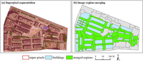
Section 2.2 presents methods for calculating only the spatial relationships between individual buildings. Previous research has predominantly focused on these spatial relationships and often overlooked the relationships among building groups. This phenomenon arises due to the exclusive depiction of buildings as graphical elements in an experimental topographic map, neglecting the visual spaces that exist between them (e.g. the green area in Figure 4). Moreover, building group patterns are often limited to building blocks (e.g. Figure 4), where roads or pathways remain conspicuously absent from the visual representation of a topographic map. Research on the recognition of building groups has not focused on the spatial relationships between building groups. This paper aims to address this gap by extracting merged regions that represent group relationships from images through image segmentation. These extracted relationships will then be employed to partition building groups across various scales. Through the application of image segmentation techniques, visual spaces are converted into a series of image merged regions. During the image segmentation process, building data may be utilized as ancillary information to facilitate the merging of regions. The methodology is structured into two primary procedures: the superpixel segmentation of image data (Section 2.3.2) and region merging (Section 2.3.3).

Figure 4. Building blocks and visual areas between building group patterns.

2.3.2. Superpixel segmentation of image data

Superpixel segmentation is the process of dividing an image into a series of homogenous regions (Hu et al. 2013). Given that the boundaries of super pixels effectively capture the contours of objects, merging them in accordance with specific criteria can result in the extraction of desired objects. Superpixel segmentation algorithms include mean clustering (Van den Bergh et al. 2015), mean shift (Achanta et al. 2012), and watershed algorithm (Hu et al. 2015). The watershed algorithm, in particular, is widely employed in region merging for its high efficiency, precise boundary detection, and superior representation of details (Hu et al. 2015, 2016). Consequently, in this article, we utilized a spatial-constrained watershed algorithm (SCoW) for our superpixel segmentation (Hu et al. 2015). The SCoW requires three parameters: λ controls the weight of spatial constraint, α balances spatial constraint and image edges, and w determines the superpixel size. Based on prior research and our own tests, we selected parameter values of λ = 0.4, α = 15, and w = 13 for our experiment. As the algorithm is published online, it will not be detailed further in this paper.

2.3.3. Region merging

To achieve the desired merged image regions, it is essential to merge the superpixels of image data. The relationship between building groups is conveyed through these merged regions; therefore, the region merging strategy involves merging along pathway directions while maintaining the compactness of the merged regions. This process solely requires consideration of the geometric shape of the merged areas. Since the spaces between building clusters are often narrow and rectangular, compactness and elongation rate serve as metrics to evaluate these two aspects. Compactness is geared toward guiding the region merging in a way that favors rectangular shapes, while the elongation ratio directs the merged regions to follow the pathways’ orientation. Finally, a weighted sum of these two indicators are calculated.

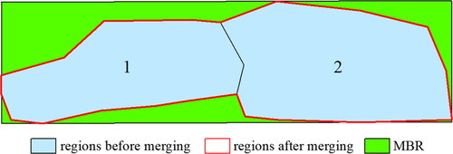
Compactness is expressed by the ratio of the sum of the areas of two regions to the minimum enclosing rectangle area of the merged region (Figure 5 and Equation 5(5) $$C=C_{i,j}=\frac{A_i+A_j}{A_{\mathit{\text{mbr}}}}$$(5) ). (5) $$C=C_{i,j}=\frac{A_i+A_j}{A_{\mathit{\text{mbr}}}}$$(5) where $C_{i,j}$ represents the compactness of a merged region derived from regions i and j, $A_i$ and $A_j$ represent the areas of region i and region j, respectively, and $A_{\mathit{\text{mbr}}}$ represents the area of the minimum bounding rectangle of the merged region. The domains of the $C_{i,j}$ are (0,1].

Figure 5. Results before and after superpixel merging.

The elongation rate is defined as the ratio of the perimeter of the merged region to its minimum bounding rectangular (MBR) area (Figure 5 and Equation 6(6) $$E=E_{i,j}=\frac{L_{\mathit{\text{merge}}}}{A_{\mathit{\text{mbr}}}}$$(6) ). (6) $$E=E_{i,j}=\frac{L_{\mathit{\text{merge}}}}{A_{\mathit{\text{mbr}}}}$$(6) where $E_{i,j}$ represents the elongation rate of the merged region derived from regions i and j, $L_{\mathit{\text{merge}}}$ represents the perimeter of the merged region, and $A_{\mathit{\text{mbr}}}$ represents the area of the minimum bounding rectangle of the merged region. The domains of the $E_{i,j}$ are (0,1).

The total cost of merging any two adjacent regions is represented as the weighted sum of the above two metrics, in accordance with Equation (7)(7) $$T{C}_{i,j}=w_{c}C+w_{e}E$$(7) . (7) $$T{C}_{i,j}=w_{c}C+w_{e}E$$(7) where $T{C}_{i,j}$ represents the total merging cost between adjacent regions i and j, $w_c$ is the weight of compactness and $w_e$ is the weight of the elongation ratio. The sum of all weights is 1.0. The larger the $T{C}_{i,j},$ the more likely the two regions are to merge.

Since the merge process is expected to perform along pathways, the elongation ratio of merged regions will become increasingly higher, necessitating a gradual increment in their weight. The weight of the elongation ratio is controlled by Equation (8)(8) $$w_e=\mathit{\text{pow}}\left(T,1.2\right)\mathrm{\hspace{0.17em}*\hspace{0.17em}}0.005+0.3$$(8) . (8) $$w_e=\mathit{\text{pow}}\left(T,1.2\right)\mathrm{\hspace{0.17em}*\hspace{0.17em}}0.005+0.3$$(8) where $w_e$ is the weight of the elongation ratio, $\mathit{\text{pow}}$ is the exponential function, $T$ signifies the multiplication of merged region area, which is calculated according to Equation (9)(9) $$T=\mathit{\text{INT}}\left(\frac{\mathit{\text{ABS}}(A-1000)}{1000}\right)$$(9) . Other constants are determined through extensive experimentation. (9) $$T=\mathit{\text{INT}}\left(\frac{\mathit{\text{ABS}}(A-1000)}{1000}\right)$$(9) where $T$ signifies the multiplication of merged region area, $\mathit{\text{INT}}$ represents the integer function, $\mathit{\text{ABS}}$ represents the absolute value function. $A$ represents the area of merged region. The constant is ascertained through numerous trials.

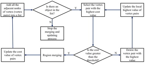
The process of region merging can be divided into three steps: merging building regions, constructing region adjacency graph (RAG), and merging and updating. Specifically, superpixels within buildings are initially merged into building regions. In this step, superpixels with more than a 50% overlap with buildings will be merged into one object. Secondly, the remaining superpixels are used to construct a RAG. In this RAG, superpixels are modeled as the vertexes of the graph, the adjacent relationships between superpixels are represented as the edges of the graph. Subsequently, merging and updating operations are performed on the graph. As regions are continuously merged, the structure of the RAG changes accordingly, necessitating constant updates to the RAG’s structure. Obviously, region merging and updating is an iterative process (Figure 6), which is conducted based on the aforementioned two indices. First, all adjacent nodes of vertexes (vertex pairs) are added to a list, and their merging cost is computed using Equation (7)(7) $$T{C}_{i,j}=w_{c}C+w_{e}E$$(7) . Then, the vertex pair with the highest cost value is selected. Third, the merging cost of the two regions is computed. If the result exceeds the threshold, the two regions are merged. Simultaneously, the local highest merging cost of vertex pairs is updated, and the process starts over from the first step. If not, the vertex pair is deleted from the list, and the local highest merging cost of vertex pairs is updated. This process is repeated until there are no vertex pairs in the list. The threshold for the merging cost is computed as per Equation (10)(10) $$\mathit{\text{CT}}=\mathit{\text{pow}}\left(T,1.5\right)\mathrm{\hspace{0.17em}*\hspace{0.17em}}0.005+0.1$$(10) . (10) $$\mathit{\text{CT}}=\mathit{\text{pow}}\left(T,1.5\right)\mathrm{\hspace{0.17em}*\hspace{0.17em}}0.005+0.1$$(10) where $\mathit{\text{CT}}$ is the threshold of merging two regions, other parameters are the same as the Equation (8)(8) $$w_e=\mathit{\text{pow}}\left(T,1.2\right)\mathrm{\hspace{0.17em}*\hspace{0.17em}}0.005+0.3$$(8) .

Figure 6. The flowchart of merging and updating process.

After extracting the merged regions, Equation (5)(5) $$C=C_{i,j}=\frac{A_i+A_j}{A_{\mathit{\text{mbr}}}}$$(5) is still used to measure the spatial continuity of two building groups connected by these merged regions. However, the triangles used for measuring the area are those connecting the buildings of the two groups.

2.4. Multiscale partitioning of building groups based on graph segmentation

In this stage, the partitioning of building groups at multiple scales is transformed into the process of graph segmentation, involving the creation and segmentation of a graph.

2.4.1. Graph creation

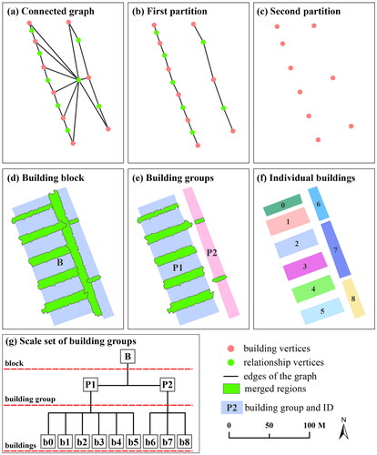
Multiscale partitioning of building groups, based on graph segmentation necessitates first creating a connected graph. All the buildings and the spatial relationships (i.e. merged regions) between building groups are modeled as a connected graph (Figure 7(a)). Thus, multiscale partitioning of building groups is tantamount to the segmentation of a graph. Figure 7(d) vividly illustrates that two potential groups are interconnected by a merged region. This merged region can be considered the vertex that connects two groups. Consequently, there are two types of vertices in the graph: building vertices and group relationship vertices. The edges of the graph represent the proximity relationship between buildings and merged regions (Figure 7(a)). Group relationship vertices are assigned a quantitative value derived from Equation (4)(4) $${\mathit{\text{SCI}}=\mathit{\text{SCI}}}_{i,j}=\frac{A_R}{A_O}$$(4) , which is used to ascertain whether a relationship vertex should be deleted during the graph segmentation process.

Figure 7. The process of graph creation and segmentation are shown for (a) graph creation; (b) the first cutting of graph segmentation; (c) the second cutting of graph segmentation; (d–f) corresponding building groups; (g) the scale set of building groups.

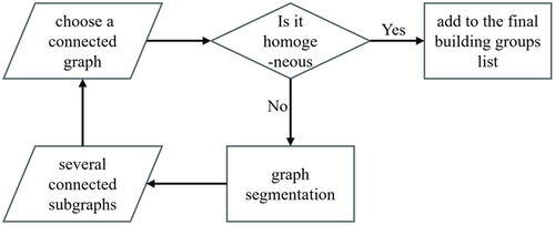
2.4.2. Graph segmentation

The process of graph segmentation is illustrated in Figure 8. This is an iterative segmentation procedure that requires constant assessment of whether the subgraphs are homogeneous. To obtain building groups at multiple scales through graph segmentation, it is essential to ensure that there is no intermediate connecting subgraph between two connected subgraphs during the segmentation process; that is, the two connected subgraphs are in a parent-child relationship. Ensuring this involves progressively removing the group relationship vertices based on their adjacency (Figures 7(a–c)). According to Equation (5)(5) $$C=C_{i,j}=\frac{A_i+A_j}{A_{\mathit{\text{mbr}}}}$$(5) , when the distance is the same, the more consistent the direction and the more similar the shape and size of neighboring objects are, the higher the SCI, and the greater the possibility that they are grouped. In addition to detecting proximity relationships, the triangles of constrained Delaunay triangulations can also indicate the distance between adjacent objects. That is, the longer the edge of a triangle is, the greater the distance between neighboring objects, and the more inconsistent the direction and area between them and vice versa. If these triangles are gradually removed, the SCI value can change significantly. The smaller the SCI value of a group relationship vertex in a graph, the earlier it is deleted. By progressively removing those relationship vertices, building groups of different scales are obtained.

Figure 8. The flowchart of graph segmentation.

Clearly, by managing the removal of triangles in the CDT, it is possible to gradually remove the relationship vertices to obtain building groups at different scales. However, if the threshold is set excessively high, relationships may be prematurely terminated, disrupting the continuity of scales within the resultant group patterns. Conversely, a deletion threshold that is too low may compromise the segmentation’s efficiency. Thus, setting a reasonable threshold is vital for the progressive segmentation of a graph. The strategy used in this study involves initially identifying the longest edge triangle within the group, the reducing this length by a specified step to define the deletion threshold for triangles. The deletion threshold determined in this manner is a dynamic threshold, as delineated in Equation (11)(11) $$L=\mathrm{\text{Max}}\left\{L_{\Delta i}^{G_j}\right\}-\alpha$$(11) . (11) $$L=\mathrm{\text{Max}}\left\{L_{\Delta i}^{G_j}\right\}-\alpha$$(11) where L is the dynamic threshold for removing triangles, $G_j$ represents the j-th building group, ${\Delta }_i$ represents the i-th triangle in the constrained Delaunay triangulation of the group, and $\alpha$ is a fixed step length.

During the process of graph segmentation, the parent-child relationships between building groups are preserved. This information, along with the average distances, facilitates the construction of a scale set for building groups (Figure 7(g)). This scale set consists of groups at different scales, allowing for the rapid retrieval of corresponding groups by a given scale parameter. In this study, we designated the scale parameter unit as meters.

2.4.3. Group homogeneity

The homogeneity of building groups is employed to ascertain the cessation of graph segmentation. It means that if the buildings within a group (i.e. a connected subgraph) exhibit exceedingly high homogeneity (e.g. similarity in terms of distance, size, and orientation), these buildings should be merged into a single object in map generalization. Otherwise, as the map is zoomed in, these buildings ought to be displayed separately (Regnauld 2001). The criteria for homogeneity are primarily based on geometric factors, such as the similarity in the size, orientation, distance, shape, and other related characteristics of buildings. Among these criteria, distance is an important metric for assessing group homogeneity (Wang et al. 2015). Moreover, distance features scalability; this characteristic indicates that the average distance between groups enlarges with increasing scale, and diminishes with decreasing scale. Hence, we utilized the standard deviation of distance as a gauge to ascertain the homogeneity of the building groups. Drawing on the findings of relevant research (Jiang and Liu 2012; Jiang et al. 2013), a threshold of 0.2 was used to ascertain the homogeneity of the groups. Furthermore, according to pertinent research and mapping standards (SAC 2006), buildings are to be depicted separately in topographic maps at scales larger than 1:2000. Human vision is capable of discerning a minimum spacing on a map of ∼0.15 mm. This minimum spacing correlates to a ground distance of 0.3 meters. Based on the analysis provided above, the stopping rule for graph segmentation is as follows: if the average distance or the standard deviation of distances of a building group (i.e. a connected subgraph) is <0.3 m and 0.2, respectively, the connected subgraph should no longer undergo partitioning.

2.5. Evaluation and method comparisons

Building group relationships, extracted from image segmentation, were validated against a manually recognized road network. To evaluate building groups obtained through multiscale partitioning, it is standard practice to perform a comparative analysis with manually obtained results (Zhang et al. 2013). This reference data is typically obtained by inviting multiple cartography experts for identification. In cases of discrepancy, a consensus is reached by a majority vote (He et al. 2020). The formula for calculating recognition accuracy is as follows: (12) $$\mathit{\text{Accuracy}}=\frac{N_a}{N_m}$$(12) where $N_a$ is the number of building groups recognized by the human visual perception process, $N_m$ represents the number of building groups detected by the automatic recognition method.

To verify the effectiveness of the proposed method, we first compared the segmentation results with those obtained from the same method but with different indicators. Furthermore, we compared the results obtained by multiscale partitioning with those derived from the method without using building group relationships. The same method with different indicators refers to the use of different elongation rates in the merging criteria. The most commonly used elongation rate indicator is the ratio of the long axis to the short axis of a rectangle (Zhang et al. 2013). The compared method did not employ building group relationships but rather used the SCI index.

The experiments were conducted on a personal computer equipped with an Intel^® Core™ i7-7700 central processing unit (CPU) and 40 GB of memory. The computer operating system is Microsoft Windows 10 (64-bit). The algorithms presented in Section 2 were implemented using C# and C++ languages on the Microsoft Visual Studio 2010 platform. These algorithms were developed utilizing the component and tool libraries provided by ArcGIS Engine 10.1.

3. Results and discussion

3.1. Multiscale building group partition results

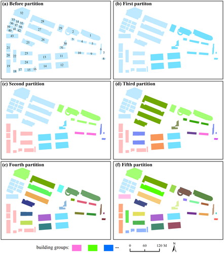
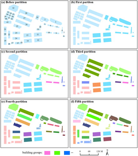
Figure 9 displays the partitioning results obtained through the suggested multiscale partitioning method. This figure illustrates only the process of group partitioning. The building groups obtained through each graph segmentation at the same level may not be those groups that can be generalized at the same scale. The proposed method partitioned all the buildings within this block five times over. Most of these results align with the human visual perception process. An error occurred in the third segmentation. Specifically, the entire building block was partitioned into two parts at the first partition (Figure 9(b)). Then, the left part was partitioned into two parts at the second partition, while the right part was partitioned into four sections due to the scattered distribution of buildings (Figure 9(c)). Building group patterns, including straight-line patterns and rectangular contour patterns, were accurately extracted during the multiscale partition process. From the first segmentation to the last, resulting in a total of 25 clusters. Compared with the reference data, 20 of them are correct groups. Thus, the proposed method has an accuracy of ∼90% in the partitioning of building groups at multiple scales.

Figure 9. The process of building group partitioning at multiple scales based on image segmentation.

Figure 10 displays the partitioning process of the comparison method based on the SCI. The initial division not only deviated from the proposed method (Figure 10(b)) but also resulted in few correct building groups in the subsequent partitions (Figures 10(c–e)). Moreover, at the fifth partition, the comparison method made a significant error by failing to group buildings 25, 26, 27, and 28 together. Because the SCI is sensitive to distance, this method is prone to errors in group partitioning when the intragroup distance exceeds the intergroup distance. Conversely, when the distances are similar, the SCI can be effectively used for identifying linear patterns (He et al. 2020). Simultaneously, McNemar test was performed on the predictions of both algorithms (Table 1). The p-value of the test is 0.001 (p < 0.01), indicating that the two methods have a statistically significant difference.

Figure 10. The process of building group partitioning at multiple scales based on the SCI.

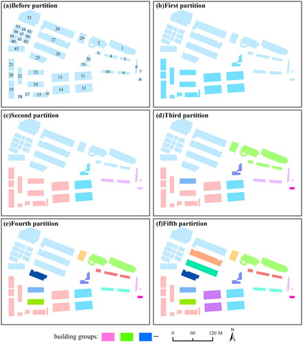
Table 1. The predictions of both methods in dataset 2.

	Comparison method correct	Comparison method incorrect
Proposed method correct	10	10
Proposed method incorrect	0	2

3.2. The scale set of building groups

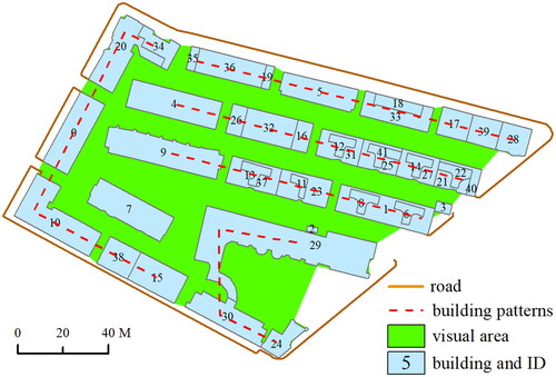
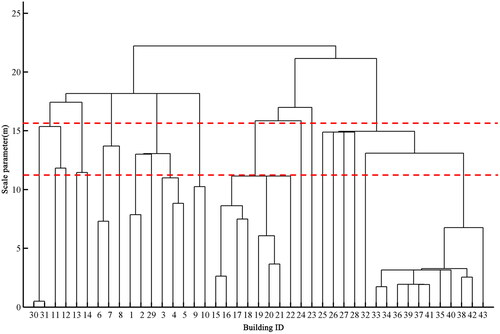
Figure 11 shows the scale set of building groups derived from the partition results of Figure 9. This figure clearly illustrates how building groups were partitioned at different scales and which groups can be generalized to express at the same scale on a map. According to the bottom of the figure, buildings 15 and 16, 20 and 21, 30 and 31, and 33–42, can be partitioned into groups at a scale of 5 m. Each of these groups can be generalized into one object. These generalized objects, along with other individual buildings, can be displayed at the same scale on a map. At a scale parameter of 20 m, only three large building groups exist. These building groups can be generalized into a single object and represented at the same scale on a map. Furthermore, it is worth noting that each group exhibited a range of expressive scales. For example, the group consisting of buildings 15 to 22 can be represented across at least five different scales (i.e. scales between two red dashed lines in Figure 11). If the scale increases, these buildings are partitioned into different groups. If the scale decreases, this group must be partitioned into several subgroups.

Figure 11. The scale set of building groups built by using the proposed method.

3.3. Superpixel segmentation and merging results

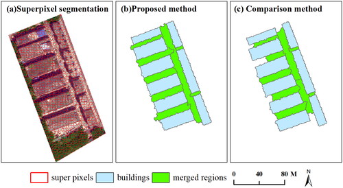
Figure 12 shows the superpixel segmentation results for experimental area 1, along with the merged results of two methods. Undoubtedly, the proposed approach not only accurately extract merged regions that serve as building group relationships, but also fully recognized the relationships between individual buildings. Visually, the longest merged region can be used to partition buildings into two groups: the left and right parts (Figure 12(b)). Conversely, the merged results obtained from the comparative method are unsatisfactory, as the comparative method cannot fully extract those merged regions used to indicate group relationships. Given that the elongation ratio does not consider the area of merged regions, the compared method may result in low compactness and irregular shapes of merged regions. Moreover, this approach negatively impacts on the subsequent merging of image regions, ultimately leading to an oversegmentation of the entire segmentation result.

Figure 12. The image segmentation and merging results are shown for (a) superpixel segmentation; (b) image merged regions of the proposed method; (c) image merged regions of the comparison method.

Figure 13 illustrates the superpixel segmentation and merged regions obtained by the proposed method for the block characterized by irregularly arranged buildings. Despite the irregular appearance of the merged regions (Figure 13(b)), they can still serve as indicators of group relationship for the purpose of multiscale partitioning of building groups. When compared to the manually extracted road network, 90% of the merged regions can be used as group relationships.

Figure 13. Superpixel segmentation and merging results in experimental area 2.

3.4. Future improvements

A crucial issue in this research is the extraction of group relationships. An optimal approach would be to solely employ vector building data to ascertain group relationships, which may minimize the need for extra laborious procedures, such as data matching. Regrettably, through extensive experimentation, we have not unveiled the challenge of utilizing vector data directly for discerning the intricate relationships among groups of buildings. The determining factors affecting the recognition of building group relationships may vary across different scenarios. These factors can include distance, shape, direction, or others. However, these factors need not be considered during image segmentation. Another rationale for employing image segmentation resides in the fact that in the event we opt for image change detection to acquire building update data, the necessity of engaging in image matching within the process of group relationship identification becomes superfluous.

Nevertheless, the proposed method still requires further refinements and improvements. First, the image regions used to indicate group relationships should be extracted more comprehensively. In our experiment, although some image regions had the potential to depict group relationships, they were mere fragments, which could impair the relationships of building groups. Improvement measures may include merging regions along the skeleton line or utilizing image merged regions as auxiliary information to recognize group relationships by using constrained Delaunay triangulations. Second, during the process of graph segmentation, the criteria for deleting relationship vertices should be more precise and reasonable. Relying solely on the SCI as the weights of relationship vertices leads to the deletion of relationships with large distances first. However, sometimes it is more appropriate to delete those relationships that are short in distance first. In other words, the relationship between groups takes precedence over that within a group. Besides distance, semantic information, such as function of buildings and the degree of road congestion should also be taken into account (He et al. 2022). As a result, the scale set of building groups established in this way may be more reasonable.

4. Conclusions

The partitioning of building groups across multiple scales forms the foundation of the multiscale transformation of buildings. Nonetheless, current research has been limited to the recognition of building groups at a single scale, making it difficult to achieve multiple representations. To address this problem, this study began with the detection of the spatial relationships between building groups. These relationships were delineated by the image merged regions derived through image segmentation. These merged regions exhibit a reliance on scales. That is, smaller merged regions are more common than larger ones. Based on these regions and buildings, a connected graph was created. Concurrently, leveraging the scaled features of these regions, we introduced a progressive partitioning approach that involves deleting the vertices represented by the merged regions to derive building groups at varying scales. The experimental results indicate that the proposed method can effectively partition building groups at different scales, achieving a partition accuracy exceeding 90%. Additionally, a scale set of building groups was built, enabling quick retrieval of specific building groups when a scale parameter is provided. These outcomes establish a robust foundation for the multiple-scale generalization of buildings and their interconnected updating, enhancing the precision and utility of building data management.

Author contributions

Conceptualization, Xianjin He and Puliang Lyu; data curation, Puliang Lyu; formal analysis, investigation, and methodology, Xianjin He; software, Xianjin He and Puliang Lyu; writing—original draft, Xianjin He; writing—review and editing, Xianjin He and Puliang Lyu. All authors have read and agreed to the published version of the manuscript.

Acknowledgements

We would like to thank the editors and the anonymous reviewers for their constructive comments.

Disclosure statement

No potential conflict of interest was reported by the author(s).

Data availability statement

Data and code are available from the corresponding author by request.

Additional information

Funding

This research was funded by the Guangxi Science and Technology Plan Project, grant numbers AD20238015 and AD20159026.

References

- Achanta R, Shaji A, Smith K, Lucchi A, Fua P, Suesstrunk S. 2012. SLIC superpixels compared to state-of-the-art superpixel methods. IEEE Trans Pattern Anal. 34(11):2274–2281.
- Ai T, Guo R. 2007. Polygon cluster pattern mining based on Gestalt principles. Acta Geod Cartogr Sin. 36(3):302–308.
- Cetinkaya S, Basaraner M, Burghardt D. 2015. Proximity-based grouping of buildings in urban blocks: a comparison of four algorithms. Geocarto Int. 30(6):618–632.
- Delong A, Osokin A, Isack HN, Boykov Y. 2012. Fast approximate energy minimization with label costs. Int J Comput Vis. 96(1):1–27. doi: 10.1007/s11263-011-0437-z.
- Deng M, Huang J, Zhang Y, Liu H, Tang L, Tang J, Yang X. 2018. Generating urban road intersection models from low-frequency GPS trajectory data. Int J Geogr Inf Sci. 32(12):2337–2361.
- Du S, Luo L, Cao K, Shu M. 2016. Extracting building patterns with multilevel graph partition and building grouping. ISPRS J Photogramm. 122:81–96.
- Du S, Shu M, Feng C. 2016. Representation and discovery of building patterns: a three-level relational approach. Int J Geogr Inf Sci. 30(6):1161–1186.
- Du S, Zhang F, Zhang X. 2015. Semantic classification of urban buildings combining VHR image and GIS data: an improved random forest approach. ISPRS J Photogramm Remote Sens. 105:107–119. doi: 10.1016/j.isprsjprs.2015.03.011.
- Guigues L, Cocquerez JP, Le Men H. 2006. Scale-sets image analysis. Int J Comput Vis. 68(3):289–317. doi: 10.1007/s11263-005-6299-0.
- He X, Deng M, Luo G. 2020. Recognizing linear building patterns in topographic data by using two new indices based on Delaunay triangulation. ISPRS Int J Geo-Inf. 9(4):231.
- He X, Deng M, Luo G. 2022. Recognizing building group patterns in topographic maps by integrating building functional and geometric information. ISPRS Int J Geo-Inf. 11(6):332.
- He X, Zhang X, Xin Q. 2018. Recognition of building group patterns in topographic maps based on graph partitioning and random forest. ISPRS J Photogramm. 136:26–40.
- Hu Z, Li Q, Zou Q, Zhang Q, Wu G. 2016. A bilevel scale-sets model for hierarchical representation of large remote sensing images. IEEE Trans Geosci Remote. 54(12):7366–7377.
- Hu Z, Shi T, Wang C, Li Q, Wu G. 2021. Scale-sets image classification with hierarchical sample enriching and automatic scale selection. Int J Appl Earth Obs. 105:102605.
- Hu Z, Wu Z, Zhang Q, Fan Q, Xu J. 2013. A spatially-constrained color-texture model for hierarchical VHR image segmentation. IEEE Geosci Remote Sens. 10(1):120–124.
- Hu Z, Zou Q, Li Q. 2015. Watershed superpixel. IEEE International Conference on Image Processing (ICIP); p. 349–353.
- Jiang B, Liu X, Jia T. 2013. Scaling of geographic space as a universal rule for map generalization. Ann Assoc Am Geogr. 103(4):844–855. doi: 10.1080/00045608.2013.765773.
- Jiang B, Liu X. 2012. Scaling of geographic space from the perspective of city and field blocks and using volunteered geographic information. Int J Geogr Inf Sci. 26(2):215–229.
- Kapoor S, Narayanan A. 2023. Leakage and the reproducibility crisis in machine-learning-based science. Patterns. 4(9):100804. doi: 10.1016/j.patter.2023.100804.
- Knura M. 2023. Learning from vector data: enhancing vector-based shape encoding and shape classification for map generalization purposes. Cartogr Geogr Inf Sc. 51(1):146–167.
- Li S, Cai Y. 2005. Some scaling issues of geography. Geogr Res Aust. 1:11–18.
- Mackaness W, Burghardt D, Cécile D, editors. 2014. Map generalisation: fundamental to the modelling and understanding of geographic space. In: Abstracting geographic information in a data rich world. Berlin: Springer; p. 1–15.
- Nan L, Sharf A, Xie K, Wong T, Deussen O, Cohen-Or D, Chen B. 2011. Conjoining gestalt rules for abstraction of architectural drawings. ACM Trans Graph. 30(6):185.
- Niu N, Liu X, Jin H, Ye X, Liu Y, Li X, Chen Y, Li S. 2017. Integrating multi-source big data to infer building functions. Int J Geogr Inf Sci. 31(9):1871–1890.
- Regnauld N. 2001. Contextual building typification in automated map generalization. Algorithmica. 30(2):312–333. doi: 10.1007/s00453-001-0008-8.
- SAC. 2006. Cartographic symbols for national fundamental scale maps-part 2: specifications for cartographic symbols 1:5000 & 1:10000 topographic maps. Beijing: Standards Press of China; p. 1–19.
- Sayidov A, Weibel R, Leyk S. 2020. Recognition of group patterns in geological maps by building similarity networks. Geocarto Int. 37(2):607–626.
- Shuai Y, Shuai H, Ni L. 2007. Polygon cluster pattern recognition based on new visual distance. Geoinformatics 2007: Geospatial Information Science: Society of Photo-Optical Instrumentation Engineers; p. 411–423. doi: 10.1117/12.761778.
- Steiniger S, Taillandier P, Weibel R. 2010. Utilising urban context recognition and machine learning to improve the generalisation of buildings. Int J Geogr Inf Sci. 24(2):253–282.
- Van den Bergh M, Boix X, Roig G, de Capitani B, Van Gool, L, AR. 2015. SEEDS: superpixels extracted via energy-driven sampling. Int J Comput Vis. 111(3):298–314. doi: 10.1007/s11263-014-0744-2.
- Wang Y, Zhang L, Mathiopoulos PT, Deng H. 2015. A Gestalt rules and graph-cut-based simplification framework for urban building models. Int J Appl Earth Obs. 35:247–258.
- Xie X, Bing-YungWong K, Aghajan H, Veelaert P, Philips W. 2015. Inferring directed road networks from GPS traces by track alignment. ISPRS Int J Geo-Inf. 4(4):2446–2471.
- Yan H, Weibel R, Yang B. 2008. A multi-parameter approach to automated building grouping and generalization. Geoinformatica. 12(1):73–89. doi: 10.1007/s10707-007-0020-5.
- Yan X, AT, Yang M, Yin H. 2019. A graph convolutional neural network for classification of building patterns using spatial vector data. ISPRS J Photogramm. 150:259–273.
- Yu W, Zhou Q, Zhao R. 2019. A heuristic approach to the generalization of complex building groups in urban villages. Geocarto Int. 36(2):155–179.
- Zhang F, Sun Q, Ma J, Lyu Z, Huang Z. 2023. A polygonal buildings aggregation method considering obstacle elements and visual clarity. Geocarto Int. 38(1):2266672.
- Zhang L, Hao D, Dong C, Zhen W. 2013. A spatial cognition-based urban building clustering approach and its applications. Int J Geogr Inf Sci. 27(4):721–740.
- Zhang X, Stoter J, AT, Kraak M, Molenaar M. 2013. Automated evaluation of building alignments in generalized maps. Int J Geogr Inf Sci. 27(8):1550–1571.
- Zhang X, Zeng G, Zhang Q. 2013. Urban geographic information system. Beijing: Science Press.